Multiscaling and Structure Functions in Turbulence: An Alternative Approach Mogens H. Jensen∗ Niels Bohr Institute and Center for Chaos and Turbulence Studies, Blegdamsvej 17, DK-2100 Copenhagen Ø, Denmark (January 15, 1999)
arXiv:chao-dyn/9901021v3 6 Aug 1999
We propose an alternative formulation of structure functions for the velocity field in fully developed turbulence. Instead of averaging moments of the velocity differences as a function of the distance, we suggest to average moments of the distances as a function of the velocity difference. This is like an “inverted” structure function, with a different statistics. On the basis of shell model calculations we obtain a new multiscaling spectrum.
Alternatively, we now consider the following quantities, which is denoted the distance structure functions
The understanding of intermittency effects in fully developed turbulence and the associated multiscaling spectrum of exponents, is probably the most fundamental open problem in turbulence research [1]. The traditional way of describing this is, as already suggested by Kolmogorov [2], to consider the velocity difference between two points of the turbulent state, raise this difference to the moment q, and then study the variation with respect to the distance between the two points. To improve the statistics, the moments are averaged in space (and maybe time) and one obtains the well known structure functions where the corresponding scaling exponents are called structure function exponents [1]. During the last decades it has become clear both from many experimental [3–5], numerical [6] and theoretical considerations [7,8], that this set of exponents is very non-trivial, defining an infinity of independent exponents leading to at “curved” variation of the scaling exponent with the moment. Notable is also the recent fundamental advances in obtaining the multiscaling spectrum analytically for a passive scalar advection in a spatially correlated, but temporally non-correlated, velocity fields, the socalled Kraichnan model [9,10] . We propose simply to “invert” the structure function equation, and consider instead averaged moments of the distance between two points, given a velocity difference between those points. This leads to an alternative way of describing and analyzing a turbulent velocity field (in particular when measured experimentally) and one obtains a new set of exponents that we have not yet been able to relate to the traditionally estimated exponents, though we suspect that there might be a relation. This inversion is inspired by studies in passive scalar advection where one often, say for pair particles, considers averages of the advection time versus the distance, instead of averages of the distance versus time [11–14]. To a start let us introduce the well known structure functions for the velocity field u(x, t) of a fully developed turbulent state, obtained either from the Navier-Stokes equations or from measurements < ∆ux (ℓ)q >∼ ℓζq
< ℓ(∆ux )q >∼ |∆ux |δq
where the difference ∆ux is again defined as in Eq. (2) and ℓ(∆ux ) is understood as the minimal distance in r, measured from x, for which the velocity difference exceeds the value ∆ux . In other words, we fix a certain set of values of the velocity difference ∆ux . Starting out from the point x, we monitor the distances ℓ(∆ux ) where the velocity differences are equal to the prescribed values. Performing an average over space (and maybe time) the distance structure functions Eq. (3) are obtained. By assuming self-similarity of the small scale velocity differences, one expects a trivial set of exponents δq where the variation with the moment q is determined by one exponent. Say, in the standard Kolmogorov theory we know that the velocity differences behave as ∆u ∼ ℓ1/3 , forgetting for a moment the averaging brackets. Inverting this equations, we of course obtain ℓ ∼ ∆u3 and would expect a trivial relation δq = 3q. In case of an intermittent and singular velocity field without self-similarity of the small scale velocity differences (see [15]), this would be completely different and the averaging brackets will be crucial, relating to the statistics of the varying quantity that is averaged. We will show, based on shell model calculations, that in turbulence there exists a new spectrum δq , that appears not to be trivially related to the spectrum ζq [16,17]. Let us for a moment reflect on the case q = 1. Using the standard value ζ1 ∼ 0.38 − 0.40, the simple inversion gives δ1 ∼ 2.5. Our calculations indicate that this value is not obtained in a turbulent model field. Instead we find a value δ1 ∼ 2.0 − 2.1. Another way to do the comparison is to aim at velocity exponent 1 and find the corresponding moment qˆ, i.e. < ℓqˆ >∼ ∆u1 . We obtain qˆ ∼ 0.45, again different from 0.40. These differences are of course attributed to the very different statistics, i.e. whether the velocity differences or the corresponding distances are averaged. Also, we obtain strong intermittency corrections in the sense that the value of the 8’th moment is ζ8 ∼ 12.9, i.e. much smaller than 8ζ1 ∼ 16.3. In order to apply this scheme in a direct calculation we employ the Gledzer-Ohkitani-Yamada, GOY, shell model [18,19] which has be intensively studied over the last years [20–26]. This model is a rough approximation to the Navier-Stokes equations and is formulated on a discrete set of k-values, kn = rn . We use the standard value r = 2. In term of a complex Fourier mode, un , of the velocity field the model reads
(1)
where the difference is defined as ∆ux (ℓ) = u(x + r) − u(x) , ℓ = |r|
(3)
(2)
The average in Eq.(1) is over space (and maybe time) . We have assumed full isotropy of the velocity field. The set of exponents ζq forms a multiscaling spectrum [7]. 1
(
d bn ∗ + νkn2 ) un = i kn (an u∗n+1 u∗n+2 + u u∗ + dt 2 n−1 n+1 cn ∗ u u∗ ) + f δn,4 , (4) 4 n−1 n−2
value ǫ = 1/2, if helicity conservation is also demanded [23]. The set (4) of N coupled ordinary differential equations can be numerically integrated by standard techniques. We have used standard parameters in this paper N = 27, ν = 10−9 , k0 = 0.05, f = 5 · 10−3 .
with boundary conditions b1 = bN = c1 = c2 = aN −1 = aN = 0. f is an external, constant forcing, here on the forth mode.
4
1
1/3 q
(a)
3.5 3 (a) ζq
2.5
0.1
2
1.5 1 0.5
0.01
0 0
2
4
6
8
10
q 0.001 1e-06 1e-05 0.0001 0.001 0.01 l
0.1
1
25
δ1q
(b) 20
100 15
(b) δq
10 1
10
0.1 5
0.01 0.001
0
0.0001
0
2
4
1e-06 0.001
0.01
1e+30
8
10
(c)
The GOY model is defined in k-space but our formalism is written in direct space and we therefore apply a sort of inverse Fourier transform [27]. Here we employ an idea proposed by Vulpiani [28,29] and write the threedimensional velocity field in the following way
1e+10
8
FIG. 2. a): The exponents ζq for the velocity structure functions, with selected error bars. The line corresponds to Kolmogorov theory. b): The exponents δq for the distance structure functions. The line is adjusted to pass through the value of the first order exponent (1, δ1 ).
0.1 |∆ux(l)|
1e+20
6 q
1e-05
1 1e-10 1e-20 1e-30 0.001
0.01
u(x, t) =
0.1
N X
cn [un (t)eikn ·x + c. c.]
(5)
n=1
|∆ux(l)|
FIG. 1. a): The velocity structure function of order one. The line has a slope of 0.39. b): The distance structure function of order one. The line has a slope of 2.02. Note the inner cut-off related to the dissipative cut-off in a), and the outer cut-off given by velocity of the forcing scale. c): The distance structure function of order 8. The exponent is δ8 ∼ 13.1. The “raggedness” is due to discretization of the varying length scale.
The wavevectors are defined by kn = kn en
(6)
where en is a unit vector in a random direction, for each shell n. Also cn are unit vectors in random directions. One can easily ensure that the velocity field is incompressible, div u = 0, by the following constraint [28] cn · en = 0
The coefficients of the non-linear terms must follow the relation an + bn+1 + cn+2 =P 0 in order to satisfy the con2 servation of energy, E = n |un | , when f = ν = 0. The constraints still leave a free parameter ǫ so that one can set an = 1, bn+1 = −ǫ, cn+2 = −(1 − ǫ) [24]. As observed by Kadanoff, one obtains the canonical
∀n
.
(7)
PN Note, that this condition could be relaxed to n=1 cn · en = 0. In our numerical computations we consider the vectors cn and en quenched in time but nevertheless average over many different realizations of these; i.e. one, 2
good precision, δ1 = 2.02 ± 0.05, with a scaling regime of 2 decades on the ∆0 u axes and 4-5 decades on the ℓ axes. Note, the cut-off at low values of ∆0 u. This cut-off is related, both for values of velocity and distance, to the dissipative cut-off of the standard structure function, see Fig. 1a. The cut-off at large values of ∆0 u is related to the velocity at the forcing scale. In all the presented calculations we have averaged over 24630 situations. Fig. 1c presents the distance structure function of order q = 8, resulting in an exponent δ8 = 12.9 ± 0.5. The graph is “rough” due to the binning of ∆0 u and due to the high moment. Fig. 2b shows the multiscaling spectrum of δq . We have included a straight line through the point (1, δ1 ) in order to show the curved nature of the spectrum. For completeness, Table 1 also displays the measured scaling exponents δq . It is well known, that one can improved the scaling significantly using the technique of extended self similarity (ESS) [31] where one moment of a given variable is varied against another moment. In the present case this means a graph of one distance structure function < ℓ(∆0 )q > ′ versus another < ℓ(∆0 )q > for two different moments ′ q, q , and this results in ESS plots which spans over three times as long a regime as compared to traditional ESS plots where the quantities are < ∆ux (ℓ)q > are applied (the large regime is of course due to the Kolmogorov 31 exponent relation). Applying ESS we have obtained the exponents δq in an independent way and the results agree well with the values listed in Table 1. This property of a much larger scaling regime of the ESS plots could be one of the advantages of the presented formalism. Details will be given in a forthcoming publication. To obtain a better understanding of the obtained results we need to consider the statistics of ℓ(∆ux )q in the following way Z < ℓ(∆ux )q >≃ ℓ(∆ux )q P (ℓ(∆ux )|∆ux ) dℓ (8)
or several, specific measurements of the distance structure functions are performed with one realization of the vectors. After that a new realization of en , cn is applied in order to perform a good statistical average.
1.2 (a)
P(l(∆ux)|∆ux)
1 0.8 0.6 0.4 0.2 0 0
0.0002
0.0004 0.0006 l(∆ux)
0.0008
0.001
1.2 (b)
P(l(∆ux)|∆ux)
1 0.8 0.6 0.4 0.2 0 0
0.5
1
1.5 l(∆ux)
2
2.5
3
FIG. 3. Probability distribution functions P (ℓ(∆ux )|∆ux ) for (a) the velocity ∆ux = 0.0027, which is close to the dissipative length scale (see Fig.1), and for (b) the velocity ∆ux = 0.26, close to the velocity of the outer cut-off.
Equipped with a real space time dependent velocity field we start out with a test of this field by computing the standard velocity structure functions, given by Eq. (1) [30]. Indeed, the field exhibits nice scaling invariance as shown in Fig.1a, where the first order velocity structure function is presented. We have extracted all the exponents with moment up to q=10 and the corresponding results are shown in Fig.2a (and for completeness also in Table 1). These results agree with the exponents obtained by numerical computations of the GOY-model in k-space [20], i.e. without performing the transformation to real space. In the averaging, we have assumed isotropy and for practical convenience, the distance is varied only along the three coordinate axes. Having checked this we proceed to extract the distance structure functions, Eq. (3). Practically, both the distance and velocity differences are discretized as ℓ = λid and ∆u = λju . In the present calculations the value λd = λu = 1.02 is chosen. As the starting point we set x = 0 and vary again along the coordinate axes. For a fixed value of ∆u0 , ℓ is increased until for the first time the velocity difference exceeds this fixed value: this defines ℓ(∆0 u). Then ∆u0 is increased by one more step and so on. Fig.1b presents the scaling of the first order distance structure function and the corresponding exponent δ1 is estimated to a rather
where we have introduced the conditional probability distribution function P (ℓ(∆ux )|∆ux ). This measures the probability of a distance ℓ given the velocity difference. We show this PDF for two different values of the velocity difference in Fig. 3 on linear scales. In both cases, the distributions are clearly non-Gaussian with long exponential (or in fact stretched exponential) tails, as expected in intermittent systems. The surprising difference to the standard PDF’s for velocity differences is, that it does not tend towards a Gaussian for large scales. We would have expected that. We have not been able to relate this PDF, P (ℓ(∆ux )|∆ux ), to the “usual” PDF, P (∆ux |ℓ); these two PDF’s measure simply very different things. In conclusion, we have introduced the distance structure functions defined for a velocity field in fully developed turbulence. The corresponding multiscaling spectrum appears not to be related to the well known spectrum for velocity structure functions. The distance structure function could be very relevant for experimental velocity data measured in one point [17]. Here one typically applies the Taylor hypothesis in order to relate a tempo3
ral segment to a spatial segment. For this type of time series, the distance structure functions should be easily extracted. I am grateful to J. Sparre Andersen, L. Biferale, P. Muratore-Ginanneschi, M. Vergassola and A. Vulpiani for comments and discussions.
[17] [18] [19] [20] [21] [22]
Electronic Address:
[email protected] [1] U. Frisch, “Turbulence: The legacy of A.N. Kolmogorov”, Cambridge University Press (1995). [2] A.N. Kolmogorov, C.R. Acad. Sci. USSR 30, 301; ibid 32, 16 (1941). [3] F. Anselmet, Y. Gagne, E.J. Hopfinger and R.A. Antonia, J. Fluid Mech. 140, 63 (1984). [4] C.M. Meneveau and K.R. Sreenivasan, Nucl. Phys. B Proc. Suppl.2 49 (1987); C.M. Meneveau and K.R. Sreenivasan, P. Kailasnath and M.S. Fan, Phys. Rev.A41, 894 (1990). [5] J. Herweijer and W. van de Water, Phys. Rev. Lett. 74, 4653 (1995). [6] A. Vincent and M. Meneguzzi, J. Fluid Mech. 225, 1 (1991). [7] R. Benzi, G. Paladin, G. Parisi and A, Vulpiani, J. Phys. A 17, 3521 (1984); G. Paladin and A. Vulpiani, Phys. Rep. 156, 147 (1987). [8] V.I. Belinicher, V.S. L’vov and I. Procaccia, Phys. Rev. E., in press (1998). [9] K. Gawedzki and A. Kupiainen, Phys. Rev. Lett. 75, 3834 (1995). [10] M. Chertkov, G. Falkovich, I Kolokolov and V. Lebedev, Phys. Rev. E 52, 4924 (1995). [11] V. Artale, G. Boffetta, A. Celani, M. Cencini and A. Vulpiani, Phys. Fluids A 9, 3162 (1997). [12] U. Frisch, A. Mazzino and M. Vergassola, Phys. Rev. Lett. 80, 5532 (1998). [13] O. Gat, I. Procaccia and R, Zeitak, Phys. Rev. Lett. 80, 5536 (1998). [14] G. Boffetta, A. Celani, A. Crisanti and A. Vulpiani, preprint chao-dyn/9807026 (1998). [15] U. Frisch, Proc. R. Soc. (London) A 434, 89 (1991). [16] Within the assumption of a multifractal model one can relate the two sets of exponents (M. Vergassola, private communication): If ∆u ∼ ℓh where h is obtained on the ∗
[23] [24] [25] [26] [27]
[28] [29]
[30] [31]
fractal set D(h) one has ζp = minh [ph+3−D(h)]. Assuming the same distribution in the two cases, an inversion leads to δq = minh [(q + 3 − D(h))/h]. L. Biferale, M. Cencini, D. Vergni and A. Vulpiani, preprint (1999). E. B. Gledzer, Sov. Phys. Dokl. 18, 216 (1973). M. Yamada and K. Ohkitani, J. Phys. Soc. Japan 56, 4210(1987); Prog. Theor. Phys. 79,1265(1988). M. H. Jensen, G. Paladin, and A. Vulpiani, Phys. Rev. A 43, 798 (1991). D. Pisarenko, L. Biferale, D. Courvasier, U. Frisch, and M. Vergassola, Phys. Fluids A 65, 2533 (1993). R. Benzi, L. Biferale, and G. Parisi, Physica D 65, 163 (1993). L. Kadanoff, D. Lohse, J. Wang, and R. Benzi, Phys. Fluids 7, 617 (1995). L. Biferale, A. Lambert, R. Lima, and G. Paladin. Physica D 80, 105 (1995). L. Kadanoff, D. Lohse, and N. Sch¨ orghofer, Physica D 100, 165 (1997). N. Sch¨ orghofer, L. Kadanoff, and D. Lohse, Physica D 88, 40 (1995). We have also tested the formalism in k-space but obtain less good statistics compared to the real space calculation. Nevertheless, by introducing a large number of shells which are less separated, say N ∼ 1000 and kn = 1.05n , the k-space computation can be pursued with good results. A. Vulpiani, private communication. T. Bohr, M. H. Jensen, G. Paladin, and A. Vulpiani, “Dynamical systems approach to turbulence”, Cambridge University Press, Cambridge (1998). The formalism has been applied to real experimental velocity fields using exit times in [17]. R. Benzi, S. Ciliberto, R. Tripiccione, C. Baudet and S. Succi, Phys. Rev. E 48, R29 (1993).
TABLE I. Values of the scaling exponents for velocity structure functions ζq and distance structure functions δq with selected error bars. q 1 2 3 4 5 6 7 8 ζq 0.39 0.73(2) 1.0 1.28(5) 1.53 1.77(6) 2.0 2.20(8) δq 2.04 3.70(5) 5.4 7.0(2) 8.53 10.0(4) 11.7 12.9(6)
4