Dec 27, 2011 - Multivariate multiscale entropy: A tool for complexity analysis of multichannel data. Mosabber Uddin Ahmed and Danilo P. Mandic. Department ...
PHYSICAL REVIEW E 84, 061918 (2011)
Multivariate multiscale entropy: A tool for complexity analysis of multichannel data Mosabber Uddin Ahmed and Danilo P. Mandic Department of Electrical and Electronic Engineering, Imperial College London, London SW7 2AZ, United Kingdom (Received 28 April 2011; revised manuscript received 12 October 2011; published 27 December 2011) This work generalizes the recently introduced univariate multiscale entropy (MSE) analysis to the multivariate case. This is achieved by introducing multivariate sample entropy (MSampEn) in a rigorous way, in order to account for both within- and cross-channel dependencies in multiple data channels, and by evaluating it over multiple temporal scales. The multivariate MSE (MMSE) method is shown to provide an assessment of the underlying dynamical richness of multichannel observations, and more degrees of freedom in the analysis than standard MSE. The benefits of the proposed approach are illustrated by simulations on complexity analysis of multivariate stochastic processes and on real-world multichannel physiological and environmental data. DOI: 10.1103/PhysRevE.84.061918
PACS number(s): 87.18.−h, 05.45.Tp, 89.75.Da
I. INTRODUCTION
Recent advances in multimodal sensing have highlighted the need for more insight into the dynamical properties of the complex phenomena under observation. The literature related to nonlinear and attractor dynamics is extensive and typically each nonlinear analysis measure focuses on one particular aspect of the data, such as complexity, dimensionality, regularity or irregularity, randomness, predictability, self-similarity, and synchrony. Among them, the time-delay embedded reconstruction [1] provides a general framework for the estimation of invariant quantities (in terms of smooth transformations of the state space of the attractor) of the original system, such as attractor dimensions, Lyapunov exponents, and entropies [2,3].1 Information theoretic measures of structural complexity include effective measure complexity (EMC) [4,5], excess entropy [6], and predictive information [7].2 However, there is neither a unique way of defining complexity rigorously, nor is it used in a consistent way in the literature. Some authors consider any signal that is not constant or periodic as complex, while most agree that neither strictly periodic nor completely random processes should be deemed complex [2]. For example, traditional entropy-based complexity measures, such as Shannon entropy [8], Kolmogorov-Sinai (KS) entropy [9], approximate entropy (ApEn) [10], and sample entropy (SampEn) [11], are maximized for random sequences—they thus suggest higher structural complexity for randomized surrogate time series than for the original one. This is misleading, especially when the signal comes from more complex systems, with pronounced correlation structures over multiple spatio-temporal scales. In 2002, Costa et al. [12] introduced the multiscale entropy (MSE) method to help resolve this issue by defining a quantitative measure of complexity that is small for both deterministic (predictable) and uncorrelated random (unpredictable) signals and large for correlated (linear and/or nonlinear) stochastic
1
A practical implementation of most of the methods can be found in the free software package TISEAN [36], publicly available at http://www.mpipks-dresden.mpg.de/∼tisean/. 2 For a comparative classification of complexity measures, see Ref. [37] and references therein. 1539-3755/2011/84(6)/061918(10)
processes, when evaluated over larger scales. This is in agreement with the consensus that the notion of dynamical complexity spans a whole range between the properties of perfect regularity and total randomness. Multiscale entropy analysis is based on evaluating at multiple time scales the sample entropy, a refinement of approximate entropy that measures the degree of randomness (or inversely, the degree of orderliness) of a time series. Historically, correlation entropy was developed to distinguish between deterministic systems by rates of information generation and was not developed for applications on stochastic data. In contrast, in Ref. [10] Pincus introduced approximate entropy as a regularity statistic to distinguish between finite, noisy, possibly stochastic (or composite deterministic), and truly stochastic data sets. It represents the conditional probability that sequences that are close (in the sense of some metric) to one another over m consecutive data points will still exhibit similarity when one more data point is added. Approximate entropy was constructed along similar lines as the correlation entropy but it has a different aim: to provide a widely applicable and statistically valid entropy formula. The justification is that if joint probability measures for reconstructed dynamics that describe the two systems are different, then their marginal probability distributions for a fixed partition, given by aforementioned conditional probabilities, are likely to be different too. As a result, using approximate entropy one needs orders of magnitude less points to accurately estimate these marginal probabilities as compared to the number of points needed to accurately reconstruct the attractor measure, as is the case with correlation entropy. Approximate entropy is applicable to noisy, typically short, real-world time series and unlike the correlation entropy, it can distinguish between correlated stochastic processes. Sample entropy is a modification of approximate entropy, and is based on the definition of the distance between two vectors in a maximum norm sense, when self-matches are excluded. As such, it represents an unbiased estimator, which is largely independent of the length of the time series. Standard entropies are based on a one-step difference (e.g., Hn+1 − Hn ) and hence do not account for features related to structure and organization over a range of time scales, other than the shortest one. To that end, multiscale entropy analysis aims at quantifying the interdependence between entropy and
061918-1
©2011 American Physical Society
MOSABBER UDDIN AHMED AND DANILO P. MANDIC
PHYSICAL REVIEW E 84, 061918 (2011)
scale, achieved by evaluating sample entropy of univariate time series coarse grained at multiple temporal scales. This facilitates the assessment of the dynamical complexity of a system; in biology this is associated with the ability of living systems to adjust to a changing environment. The underlying integrative multiscale functionality is interpreted by nondiminishing entropy values across increasing time scales. A detailed analysis of MSE for correlated and uncorrelated noises with Gaussian and inverse Gaussian distributions can be found in Refs. [13] and [14]. There exist several improvements of MSE, especially regarding the definition of the time scales [15–17], contributing to its theoretical foundations. The method has been successfully applied across biomedical research, such as in fluctuations of the human heartbeat under pathologic conditions [12], EEG and MEG in patients with Alzheimer’s disease [18], complexity of human gait under different walking conditions [19], variations in EEG complexity related to aging [20], and human red blood cell flickering [21]. These results strongly support the general complexity-loss theory for systems under stress, for instance, through aging and disease [22]. The existing MSE algorithm has been designed for the analysis of scalar time series, and is not suited for multivariate time series that are routinely measured in experimental and biological systems. Standard MSE treats multivariate time series as a set of individual time series by considering each variable separately, however, this is only applicable if all the data channels are statistically independent or uncorrelated at the very least (which is often not the case). For example, measurements of the z coordinate of the Lorenz system cannot reconstruct the dynamics of the Lorenz system, because they do not resolve the x-y symmetry [23]. In addition, there are substantial advantages in simultaneously analyzing several variables observed from the same phenomenon, especially if there is a large degree of uncertainty and coupling underlying the system dynamics or data acquisition. The multivariate extension of MSE in this work is based on our definition of multivariate sample entropy (MSampEn). The proposed multivariate MSE (MMSE) evaluates MSampEn over different time scales and deals with the different embedding dimensions, time lags, and amplitude ranges of data channels in a rigorous and unified way. The method is shown to cater for linear and/or nonlinear within- and cross-channel correlations as well as for complex dynamical couplings and various degrees of synchronization over multiple scales, thus allowing for direct analysis of multichannel data. The advantages of the proposed multivariate approach, in contrast to analyzing each data channel separately, are illustrated for both synthetic stochastic processes and real-world gait, wind, and physiological data. II. MULTIVARIATE MULTISCALE ENTROPY
The multivariate multiscale entropy (MMSE) analysis is performed through the following two steps: (i) Define temporal scales of increasing length by coarse graining the multivariate time series {xk,i }N i=1 ,k = 1,2, . . . ,p, where p denotes the number of variates (channels) and N the number of samples in each variate. Then, for a scale factor �,
the elements of the multivariate coarse-grained time series are calculated as � = yk,j
j� 1 � xk,i , � i=(j −1)�+1
(1)
where 1 � j � N� and k = 1, . . . ,p. (ii) Calculate the multivariate sample entropy, MSampEn, � for each coarse-grained multivariate yk,j , and plot MSampEn as a function of the scale factor �. Multivariate sample entropy is therefore a prerequisite for performing multiscale entropy (MMSE) analysis simultaneously over a number of data channels. Recall from multivariate embedding theory [23] that the multivariate embedded reconstruction for a p-variate time series {xk,i }N i=1 ,k = 1,2, . . . ,p generated from the same system and observed through p measurement functions hk (yi ), is based on the composite delay vector Xm (i) = [x1,i ,x1,i+τ1 , . . . ,x1,i+(m1 −1)τ1 , x2,i ,x2,i+τ2 , . . . ,x2,i+(m2 −1)τ2 , . . . , xp,i ,xp,i+τp , . . . ,xp,i+(mp −1)τp ],
(2)
where M = [m1 ,m2 , . . . ,mp ] ∈ Rp is the embedding vector, m τ = [τ� 1 ,τ2 , . . . ,τp ] the time lag vector, and Xm (i) ∈ R p (m = k=1 mk ). For illustration, consider a wind signal recorded using a two-dimensional (2D) anemometer, where the wind speed time series from the east-west and north-south directions are denoted respectively by x(t) = {x1 ,x2 , . . . ,xN } and y(t) = {y1 ,y2 , . . . ,yN }, with each time series of N data points. For the time lag vector τ = [2,1] and the embedding vector M = [2,2], some of the composite delay vectors are [x1 ,x3 ,y1 ,y2 ], [x2 ,x4 ,y2 ,y3 ], and [x3 ,x5 ,y3 ,y4 ]. Section II-B evaluates this issue further and provides a geometric interpretation. A. Multivariate sample entropy method
Richman and Moorman [11] introduced sample entropy (SampEn) as a conditional probability that two sequences of m consecutive data points, which are similar to within a tolerance level r, will remain similar when the next data point is included, provided that self-matches are not considered in calculating the probability. When extending univariate sample entropy to the multivariate case, we need to consider the following issues. First, it is important to notice that multivariate data do not necessarily have the same amplitude range among the data channels, so that the distances calculated on embedded vectors may be biased toward the variates with largest amplitude ranges. To that end, we propose to scale all the data channels to the same amplitude range, and choose the range [0,1] as a preferred choice. As shown later, other choices will not affect the multivariate sample entropy calculation. Second, for a fixed embedding dimension m, sample entropy calculates the average number of delay vector pairs that are within a fixed threshold r, and repeats the same for dimension (m + 1). There are p ways in which we can evolve from the space of dimension m described by the embedding vector [m1 ,m2 , . . . ,mk , . . . ,mp ] to any space of dimension (m + 1) described by the embedding vector
061918-2
MULTIVARIATE MULTISCALE ENTROPY: A TOOL FOR . . .
PHYSICAL REVIEW E 84, 061918 (2011)
[m1 ,m2 , . . . ,mk + 1, . . . ,mp ] where k = 1, . . . ,p is the index of data channel. It is important to notice that the average number of delay vector pairs that are within a fixed threshold for dimension (m + 1) can be calculated in two ways. A naive approach would be, if for each of the k-th subspaces of the (m + 1)-dimensional space, we calculate the average number of delay vector pairs that are within a fixed threshold, and then average over all the p subspaces. A rigorous approach would be to take into account all the delay vectors in all the subspaces and then compare the delay vectors both within and across the p subspaces. This way, along with time correlations, we have means to cater for linear and/or nonlinear spatial correlations. This is crucial in situations where the measurements come from similar physical quantities, simultaneously recorded at different positions in a spatially extended system, as in the case of geophysical sensors or scalp EEG. For heterogeneous data channels (i.e., heartbeat interval series and respiratory signals), this makes it possible to cater for the dynamical couplings and various degrees of synchronization over multiple scales. Third, as sample entropy is a relative measure and the threshold parameter is set as some percentage of the standard deviation of the observed time series, we also need a multivariate generalization of the univariate notion of variance. Though the covariance matrix, S, is one such generalization, we still need a single number to measure the multivariate scatter in the data. Two such common measures are the generalized variance, |S|, and the total variation, tr(S); in this work we use total variation. To maintain the same total variation for all the multivariate series under consideration, we normalize each data channel to unit variance so that the total variation becomes equal to the number of channels or variables. This way, differences in the variance among the multivariate time series under consideration do not influence the calculation of multivariate sample entropy. Finally, in univariate approximate (sample) entropy methods, the time delay, τ , is not used as a parameter (a unit time delay is assumed), thus assuming that the phase-space representation of a time series is independent of the value of the time lag τ . However, this is only the case for an infinite amount of data. In digital signal processing, both embedding dimension, m, and time lag, τ , ought to be considered for determining the optimal tap input length of an adaptive filter or a time-delay neural network. For instance, if the temporal span (m × τ ) is too small, the signal variation within the delay vector is largely governed by noise and either m or τ should be increased. There is no established criterion for choosing which of the two parameters to modify, and it is common to have a fixed time lag τ (sampling rate) and to adjust the embedding dimension m (length of a filter) accordingly. In the multivariate case, different observed variables are likely to have different embedding dimensions and time lags, and we need to use different mk and τk values for different channels or variables. In our approach, both M and τ are varying (vector parameter) and can be optimized either separately or simultaneously [24]. Multivariate sample entropy calculation. For a p-variate time series {xk,i }N i=1 ,k = 1,2, . . . ,p, we introduce MSampEn through the following procedure: (i) Form (N − n) composite delay vectors Xm (i) ∈ Rm , where i = 1,2, . . . ,N − n and n = max{M} × max{τ }.
(ii) Define the distance between any two composite delay vectors Xm (i) and Xm (j ) as the maximum norm [25], that is, d[Xm (i),Xm (j )] = maxl = 1,...,m {|x(i + l − 1) − x(j + l − 1)|}. (iii) For a given composite delay vector Xm (i) and a threshold r, count the number of instances Pi where d[Xm (i),Xm (j )] � r, j �= i, then calculate the frequency of 1 occurrence, Bim (r) = N−n−1 Pi , and define a global quantity B m (r) =
N−n 1 � m B (r). N − n i=1 i
(3)
(iv) Extend the dimensionality of the multivariate delay vector in (2) from m to (m + 1). This can be performed in p different ways, as from a space defined by the embedding vector M = [m1 ,m2 , . . . ,mk , . . . ,mp ] the system can evolve to any space for which the embedding vector is [m1 ,m2 , . . . ,mk + 1, . . . ,mp ] (k = 1,2, . . . ,p). Thus, a total of p × (N − n) vectors Xm+1 (i) in Rm+1 are obtained, where Xm+1 (i) denotes any embedded vector upon increasing the embedding dimension from mk to (mk + 1) for a specific variable k. In the process, the embedding dimension of the other data channels is kept unchanged, so that the overall embedding dimension of the system undergoes the change from m to (m + 1). (v) For a given Xm+1 (i), calculate the number of vectors Qi , such that d[Xm+1 (i),Xm+1 (j )] � r, where j �= i, then calcu1 late the frequency of occurrence, Bim+1 (r) = p(N−n)−1 Qi , and define the global quantity B m+1 (r) =
p(N−n) � 1 B m+1 (r). p(N − n) i=1 i
(4)
(vi) This way, B m (r) represents the probability that any two composite delay vectors are similar in dimension m, whereas B m+1 (r) is the probability that any two composite delay vectors will be similar in dimension (m + 1). (vii) Finally, for a tolerance level r, MSampEn is calculated as the negative of a natural logarithm of the conditional probability that two composite delay vectors close to each other in an m dimensional space will also be close to each other when the dimensionality is increased by one, and is given by � m+1 � (r) B MSE (M,τ ,r,N ) = −ln . (5) m B (r) where the symbol MSE denotes MSampEn. B. Geometric Interpretation
Figure 1 illustrates the principle behind multivariate sample entropy calculation. Consider a two-dimensional recording of wind speed, shown in Fig. 1(a), where the eastward component is denoted by x(t) (solid blue line) and the northward component by y(t) (dotted red line). Assume the time lag vector τ = [1,1] and the embedding vector M = [1,1]; then the composite delay vectors will be [x(t),y(t)] where t denotes the time index, as shown in Fig. 1(b). For any such vector (e.g., [x(64),y(64)]), we need to find the number of neighbors that are within a distance r (tolerance level), illustrated by a circle
061918-3
MOSABBER UDDIN AHMED AND DANILO P. MANDIC 3
3
Eastward wind, x(t) Northward wind, y(t)
2
circle with radius r
1
1 y(64)
0 −1
x(64)
0 −1
−2 −3 0
[x(64), y(64)]
2
y(t)
Wind speed( m/s)
PHYSICAL REVIEW E 84, 061918 (2011)
−2
50
100
150 200 Time (ms), t
250
−3 −3
300
−2
−1
0 x(t)
1
2
3
(a) Wind speed time series
(b) A 2D scatter plot of vectors [x(t), y(t)]
(c) A 3D-plot of vectors [x(t), x(t+1), y(t)]
(d) A 3D-plot of vectors [x(t), y(t), y(t+1)]
FIG. 1. (Color online) Geometry behind the calculation of MSampEn.
centered at [x(64),y(64)] with radius r. For an m-dimensional space, the set of neighboring vectors is enclosed by an m-sphere if the distance is calculated using the Euclidean norm and by an m-cube if we use a maximum distance norm. The average number of vectors that are within a fixed threshold r in this two-dimensional space is next calculated. The number of r-neighbors of an embedded vector is an estimate of the local probability density, and is also a measure of their joint probability, as all the m-components of the neighboring vector have to be simultaneously similar to those of the vector in hand. When increasing the embedding dimension m, we therefore inherently involve joint probabilities covering larger time spans. For the example in Fig. 1, upon increasing the embedding dimension from two to three, we have two subspaces of dimension three: (i) the subspace of all the vectors [x(t),x(t + 1),y(t)] [Fig. 1(c)] and (ii) the subspace of all the vectors [x(t),y(t),y(t + 1)] [Fig. 1(d)]. A naive approach would be to calculate the number of vectors that are within a fixed threshold r in each three-dimensional subspace and then average over both subspaces [26]. Instead, we employ a rigorous approach and compare composite delay vectors (to find the neighbors) not only within each subspace but also across all the subspaces, thus fully catering for both withinand cross-channel correlations. This allows us to calculate the
conditional probability that two sequences of m data points (or two composite delay vectors in m-dimensional space), which are similar to within a tolerance level r, will remain similar in the same sense, when the next data point is included (or the dimension of the composite delay vector is increased by one), provided that self-matches are not considered. A negative logarithm of this conditional probability defines the multivariate sample entropy.
III. MULTIVARIATE COMPLEXITY ANALYSIS
The multivariate MSE (MMSE) plots, that is, multivariate sample entropy represented as a function of the scale factor, are next used to assess relative complexity of normalized multichannel temporal data. The interpretation of the MMSE analysis is as follows: (i) The multivariate time series X is considered more dynamically complex than the multivariate time series Y, if for the majority of time scales the multivariate sample entropy values for signal X are higher than those for signal Y. (ii) A monotonic decrease in the multivariate entropy values with the scale factor indicates that the signal in hand only contains useful information at the smallest scales, this is typical for both completely random and fully predictable signals.
061918-4
MULTIVARIATE MULTISCALE ENTROPY: A TOOL FOR . . .
PHYSICAL REVIEW E 84, 061918 (2011) 2
Two channels contain 1/f noise, one white noise
1
0.5
0 0
Multivariate sample entropy
All three channels contain 1/f noise
All three channels contain white noise
5
One channel contains 1/f noise, others white noise 10 15 20 Scale factor
FIG. 2. (Color online) MMSE analysis for three-channel data containing white and 1/f noise, each with 10 000 data points. The curves represent an average of 20 independent realizations and error bars the standard deviation (SD).
(iii) A multivariate system exhibiting long-range correlations and complex generating dynamics is characterized by either a constant multivariate sample entropy or it exhibits a monotonic increase in multivariate sample entropy with the scale factor.3 A. Validation on synthetic data
The univariate MSE analysis has shown [12,13] that for random white noise (uncorrelated), the sample entropy values decrease monotonically with scale, whereas for a 1/f noise (long-range correlated) sample entropy remains constant over multiple time scales. This indicates that the univariate 1/f noise is structurally more complex than uncorrelated random signals. To illustrate the corresponding behavior for the multivariate case, we generated a trivariate time series, where originally all the data channels were realizations of mutually independent white noise. We then gradually decreased the number of variates that represent white noise (from 3–0) and simultaneously increased the number of data channels that represent independent 1/f noise (from 0–3), so that the total number of variates was always three. The values of the parameters used to calculate MSampEn in this section were mk = 2, τk = 1, and r = 0.15×(standard deviation of the normalized time series) for each data channel. Figure 2 shows the MMSE curves for the cases considered; notice that as the number of variates representing 1/f noises increased, MSampEn at higher scales also increased, and when all the three data channels contained 1/f noise, the complexity at larger scales was the highest. The analysis in Fig. 2 therefore confirms that, as desired, the more variables or channels within a multivariate time series exhibit long-range correlations, the higher the overall complexity of the underlying multivariate system.
3 MATLAB toolbox for the proposed MMSE method can be found at http://www.commsp.ee.ic.ac.uk/∼mandic/research/Complexity Stuff.htm.
Correlated trivariate 1/f noise Uncorrelated trivariate 1/f noise Correlated trivariate white noise Uncorrelated trivariate white noise
1.5
Correlated and uncorrelated trivariate 1/f noise 1
0.5 Correlated and uncorrelated trivariate white noise 0 0
1
2
3
4
5
6 7 8 9 10 11 12 13 14 15 Scale factor (a) Naive approach
2 Multivariate sample entropy
Multivariate sample entropy
1.5
Correlated trivariate white noise 1.5
Correlated trivariate 1/f noise
1
0.5 Uncorrelated trivariate white noise Uncorrelated trivariate 1/f noise 0 0
1
2
3
4
5
6 7 8 9 10 11 12 13 14 15 Scale factor (b) Full multivariate approach
FIG. 3. (Color online) Multivariate multiscale entropy (MMSE) analysis for trivariate white and 1/f noise, each with 10 000 data points. The curves represent an average of 20 independent realizations and error bars the standard deviation (SD).
Recall that the original univariate MSE algorithm accounts for long-term correlations within a single data channel, however, due to its univariate nature, it cannot model the cross-channel information present in multivariate recordings. On the other hand, MMSE is designed for multivariate data. To illustrate this difference, we first generated independent realizations of white and 1/f noise, and the three channels of trivariate white and 1/f noise were constructed using combinations of those independent realizations, thus making the channels correlated. Figure 3 illustrates the ability of MMSE to model both within- and cross-channel properties in multivariate data. Figure 3(a) shows that the naive multivariate approach accounts for within-channel correlations but not for cross-channel correlations, and was not able to distinguish between uncorrelated and correlated trivariate random and 1/f noises. Figure 3(b) shows that, as desired, the proposed multivariate MSE fully caters for both within- and cross-channel correlations. Indeed, based on MMSE the complexity of the correlated trivariate 1/f noise at large scales was the highest, followed by the uncorrelated 1/f noise, and correlated and
061918-5
MOSABBER UDDIN AHMED AND DANILO P. MANDIC 4
Sample entropy
3.5 3
1
AR(2) process
0
−1 2.5 0
1
AR(4) process
0
IV. APPLICATIONS FOR REAL-WORLD MULTIVARIATE PROCESSES
AR(6) process
The multivariate multiscale entropy analysis is next evaluated for three multivariate real-world recordings: human stride interval analysis, three-dimensional wind measurements from different dynamical regimes, and bivariate physiological data (breathing and heartbeats) from young and elderly subjects.
0
−1 40 0
20
1
PHYSICAL REVIEW E 84, 061918 (2011)
20
−1 40 0
20
40
2 1.5
A. Stride interval characterization
1 0.5 White noise 0 0
10
20 Scale factor
30
40
FIG. 4. (Color online) Standard univariate multiscale entropy analysis for white noise and scalar AR processes, each with 10 000 data points. The curves represent an average of 20 independent realizations and error bars the standard deviation (SD).
uncorrelated white noise. This conforms with the underlying physics and validates the proposed MMSE method, as the complexity of the considered multivariate processes exhibiting both within- and cross-channel correlations is higher than that of uncorrelated multivariate white noise and uncorrelated multivariate 1/f noise (where long-range correlations only exist within single channels). The usefulness of the MMSE analysis is further illustrated for the analysis of scalar and vector autoregressive (AR) processes [27]. The AR processes were designed so as to have an increasing correlation span with the model order. Figure 4 shows the standard univariate MSE analysis for the scalar AR processes considered and Fig. 5 the MMSE analysis for the corresponding bivariate vector AR (VAR) processes. As desired, in both cases, as the model order increased, the complexity of the corresponding signals measured by MSE and MMSE increased too.
The data used were from Ref. [28], where stride interval fluctuations were recorded from ten healthy subjects who walked for one hour at their usual, slow, and fast paces. The participants were further asked to walk following a metronome, which was set to each participant’s mean stride interval. To assess the differences in relative complexity between the unconstrained (slow, normal, fast) and the corresponding constrained (metronomically-paced) conditions, we considered the three walking paces as different variables from the same system, and used MMSE to discriminate between the self-paced and metronomically-paced walk. To test the hypothesis that the complexity of such time series is encoded into the sequential ordering of the samples of stride intervals, we also produced the corresponding surrogate time series by shuffling (randomly reordering) the sequence of data points. In this way, in surrogates the correlations among the data samples were destroyed, while preserving statistical properties of the distributions (particularly the first and second moment), and the complexity of the surrogates is lower than or equal to (if the original is completely random) that of the original signal. The values of the parameters used to calculate MSampEn were mk = 2, τk = 1 and r = 0.15×(standard deviation of the normalized time series) for each data channel; these parameters were chosen on the basis of previous studies indicating good statistical reproducibility for SampEn [11]. For MSE
SampEn
Normal condition 2 1 0 1
2
2
1.5
MSampEn
Bivariate AR(6) process Bivariate AR(4) process
MSampEn
Multivariate sample entropy
2.5
1
0.5
Bivariate white noise
0 0
5
10 Scale factor
15
20
FIG. 5. (Color online) Multivariate multiscale entropy (MMSE) analysis for bivariate white noise and bivariate AR processes, each with 10 000 data points. The curves represent an average of 20 independent realizations and error bars the standard deviation (SD).
4
5
6
7
6
7
6
7
2 1 0 1
2
3
4
5
Fast, normal and slow conditions 1.5 1 0.5 0 1
Unconstrained walking
Bivariate AR(2) process
3
Fast and normal conditions
2
3
4 Scale factor
Randomized Unconstrained walking
5
Metronomically−paced walking
Randomized Metronomically−paced walking
FIG. 6. (Color online) Multivariate multiscale entropy (MMSE) analysis for self-paced (solid red square) vs metronomically-paced (solid cyan circle) stride interval (human gait) time series and for their corresponding randomized surrogates (dashed line). Top: univariate MSE analysis; Middle: bivariate MMSE analysis; Bottom: Trivariate MMSE analysis. The curves represent an average of trials from 10 subjects and error bars the standard deviation (SD).
061918-6
MULTIVARIATE MULTISCALE ENTROPY: A TOOL FOR . . .
PHYSICAL REVIEW E 84, 061918 (2011)
or MMSE, the length of each coarse-grained sequence was � (scale factor) times shorter than the length of the original series, so the highest scale factor considered in the analysis was � = 7. The top panel in Fig. 6 shows the results obtained by the univariate MSE performed for the normal speed time series [19]—the univariate MSE was not able to perform statistically significant discrimination between the self-paced and metronomically-paced walk as the error bars overlapped. The middle and bottom panels in Fig. 6 show that when the walking conditions are considered within the multivariate approach (bivariate for any two walking conditions or trivariate for all the three walking conditions), the proposed MMSE was able to discriminate between the self-paced and metronomically-paced walk. This opens unique analysis possibilities, since the MMSE method was able to consider all the walking conditions within one unifying model, directly benefiting from the multivariate approach. Figure 6 also indicates the presence of persistent serial correlations, which are long-range dependent in self-paced walking, and the lack of any correlations in metronomically-paced walking; in this case the shape of the MMSE curve is similar to that for multivariate white noise. As expected, the surrogate series (randomly shuffled) showed a similar pattern to that for white noise (dashed line in Fig. 6). To evaluate the statistical difference of the entropy statistics between self-paced and metronomically-paced sets, the Student’s t-test and the Mann-Whitney U test (also known as Wilcoxon rank sum test) were applied. Student’s t-test is a parametric approach that tests the null hypothesis that the means of normally distributed populations are equal. On the other hand, the Mann-Whitney U test is a nonparametric test where the null hypothesis, that independent samples come from identical (similar shape) continuous (not necessarily normal) distributions with equal medians, is tested against the alternative that they do not have equal medians. Entries in Table I represent the scales at which MSampEn measures between self-paced and metronomically-paced walking are significantly different according to the above two statistical tests. When all three walking conditions were simultaneously considered, both the statistical significance tests revealed significant differences (p < 0.01) in MSampEn measures at all scales except for � = {1,2} and the corresponding null hypothesis (equal mean or median) was rejected. On the other hand, for the univariate MSE there were no statistically significant differences between self-paced walking and metronomically-paced walking at any scales. TABLE I. Statistical significance tests for the univariate, bivariate, and trivariate human stride interval analysis. Shown are scales for which the differences are statistically significant. Conditions taken Normal Fast Slow Fast and Normal Fast and Slow Normal and Slow Fast, Normal, and Slow
Student’s t-test
Mann-Whitney U test
No scale No scale No scale 6,7 4,5,6,7 5,6,7 3,4,5,6,7
No scale No scale No scale 6,7 4,5,6,7 5,6,7 3,4,5,6,7
This result also indicates that for metronomically-paced walking in slow, normal, and fast conditions, the time series share uncorrelated random underlying dynamics both withinand cross-channel, whereas for free walking, the time series for slow, normal, and fast conditions are correlated both withinand cross-channel. That explains why at larger scales the complexity for the multivariate measurements was highest for self-paced walking (compared to metronomically-paced walking), and the separation was statistically significant over more scales when we considered all the available walking conditions. The MMSE therefore offers a significant improvement over the previous studies [19,28] and also supports the more general concept of multiscale complexity loss with aging and disease or when a system is under constraints (metronomicallypaced), which all reduce the adaptive capacity of biological organization at all levels [22].
B. Complexity analysis of physiological signals
We shall now apply the MMSE method to the Fantasia database [29] to simultaneously analyze the complexity of interbeat interval (R-R) and interbreath interval series. The presence of long-range correlations in both cardiac and respiratory dynamics was previously established using detrended fluctuation analysis (DFA) in Refs. [30] and [31]. A subset of the Fantasia database was chosen consisting of ten young (21–34 years old) and ten elderly (68–85 years old) rigorously screened healthy subjects who underwent 120 minutes of continuous supine resting while continuous electrocardiographic (ECG) and respiration signals were collected. Each subgroup of subjects included seven women and three men. The continuous ECG and respiration signals were digitized at 250 Hz, and the interbeat interval (R-R) time series and interbreath interval time series were generated (for more details see Refs. [30] and [31]). The values of the parameters used to calculate MSampEn were mk = 2, τk = 1, and r = 0.15×(standard deviation of the normalized time series) for each variate. First, the univariate MSE was applied separately to the interbeat interval (R-R) series [Fig. 7(a)] and interbreath interval series [Fig. 7(b)]. For rigor, the corresponding surrogate time series were also produced by shuffling (randomly reordering) the sequence of data points. In both cases, although, as desired, for some scales physiological signals from healthy young subjects exhibited higher complexity than those of healthy elderly subjects, the complexity values were lower than those of the randomized surrogates. This behavior wrongly suggests a lack of long-term correlations in both cardiac and respiratory dynamics, illustrating that the univariate approach was not able to produce robust estimates. Next, MMSE was applied to a bivariate time series consisting of the R-R and interbreathing intervals. Figure 8 reveals long-range correlations in both cardiac and respiratory dynamics, illustrated by the fact that the MSampEn values for larger scales were higher than those of the randomized surrogates, which have no temporal structure. Figure 8 also indicates lower complexity of physiological responses of elderly subjects than the young ones, conforming with the complexity loss theory with aging [30].
061918-7
MOSABBER UDDIN AHMED AND DANILO P. MANDIC
Sample entropy
2.5
2
Randomized R−R interval series from old subjects R−R interval series from young subjects
2 1.5 1 0.5 0 0
Randomized R−R interval series from young subjects R−R interval series from old subjects
2
4
6 Scale factor
8
Sample entropy
Randomized IBI signal from young subjects IBI signal from young subjects
1
0 0
Randomized IBI signal from old subjects 2
1 Randomized bivariate 0.5 data from old subjects
2
4
Bivariate data from old subjects
6 Scale factor
8
10
FIG. 8. (Color online) Multivariate multiscale entropy (MMSE) analysis of the bivariate (R-R, interbreath interval) signal. The curves represent an average of 10 subjects and error bars the standard deviation (SD).
1.5
0.5
Bivariate data from young subjects
1.5
0 0
3
2
Randomized bivariate data from young subjects
10
(a) R-R interval series
2.5
Multivariate sample entropy
3
PHYSICAL REVIEW E 84, 061918 (2011)
IBI signal from old subjects
4
6 8 10 Scale factor (b) Interbreath interval (IBI) series
FIG. 7. (Color online) Univariate multiscale entropy (MSE) analysis for the cardiac and respiratory dynamics. The curves represent an average of 10 subjects and error bars the standard deviation (SD).
separately to data channels representing the eastward, northward, and vertical direction, as well as to the modulus of the 3D wind. For rigor, the corresponding surrogate time series were also produced by shuffling (randomly reordering) the sequence of data points. Figure 10 shows the univariate complexity profiles for the three channels and for different wind regimes. For the eastward wind [Fig. 10(a)], the high dynamics regime exhibited the highest univariate complexity, followed by the medium and low dynamics regimes. This is contrary to the intuition and the underlying physics, and is attributed to the shortcomings of univariate MSE, as it represents the variability in each univariate regime (identified in Fig. 9) and not true complexity. For the vertical wind [Fig. 10(c)], the same interpretation applies. Only the analysis of northward wind [Fig. 10(b)] and the modulus of the 3D wind [Fig. 10(d)] behaved in the expected way, that is, medium wind dynamics has fewest constraints, and is thus most complex [35] as mild winds
C. Complexity analysis of different wind regimes
5 High Absolute wind speed (m/s)
Evidence of long-range correlations in wind speed recordings exists, and was evaluated using, for example, Hurst parameters and detrended fluctuation analysis (DFA) [32–34]. We shall now illustrate that the MMSE method allows us to characterize different wind regimes in terms of the underlying dynamical complexity. The data set was recorded using a 3D ultrasonic anemometer (measurements taken in the north-south, east-west, and vertical directions) at a sampling frequency of 50 Hz in the courtyard of the Institute of Industrial Science (IIS) of the University of Tokyo. To reduce the effects of high-frequency noise, the data was preprocessed by a moving average filter. Figure 9 shows that throughout the day, the wind dynamics was changing, and the three wind regimes of different dynamics were identified and labeled as low, medium, and high. The values of the parameters used to calculate MSampEn were mk = 2, τk = 1, and r = 0.20×(standard deviation of the normalized time series), for each of the three data channels. The univariate multiscale entropy analysis was first applied
4 3 Medium 2 Low 1 0 0
1
2 3 Time (samples)
4
5 4
x 10
FIG. 9. (Color online) Magnitude of the 3D wind signal. The wind dynamics regimes are identified as low, medium, and high.
061918-8
MULTIVARIATE MULTISCALE ENTROPY: A TOOL FOR . . .
Sample entropy
4
3
2.5
Wind data from high dynamics (HD) regime Wind data from medium dynamics(MD) regime Wind data from low dynamics (LD) regime Randomized wind data from HD regime Randomized wind data from MD regime Randomized wind data from LD regime
2 Sample entropy
5
PHYSICAL REVIEW E 84, 061918 (2011)
Randomized wind data 2
Medium dynamics regime High dynamics regime
Randomized wind data 1.5 Medium dynamics regime
1
0.5
1
Low dynamics regime
0 0
Low dynamics regime 2
4
6 8 Scale factor (a) Eastward wind speed
0 0
10
2
4
High dynamics regime
6 Scale factor
8
10
(b) Northward wind speed
2.5
2.5 Randomized wind data 2 Sample entropy
Sample entropy
2 High dynamics regime 1.5
1 Medium dynamics regime 0.5
Randomized wind data 1.5
1
0.5 High dynamics regime
Low dynamics regime 0 0
Medium dynamics regime
2
4
6 Scale factor
Low dynamics regime 8
0 0
10
2
(c) Vertical wind speed
4
6 Scale factor
8
10
(d) Modulus of 3D wind speed
FIG. 10. (Color online) Univariate multiscale entropy (MSE) analysis of 3D wind speed data. The curves represent an average of six trials and error bars the standard deviation (SD).
3.5 Multivariate sample entropy
come from a wide range of directions. For each direction, the wind data showed lower complexity than their corresponding surrogate series, wrongly suggesting that the wind data set considered had no long-range correlations. Figure 11 shows the corresponding multivariate multiscale entropy analysis, performed by considering the three wind directions as variables in a trivariate model. Observe that the multivariate approach was capable of detecting long-range correlations in the wind speed for all wind regimes as the MMSE curves were similar to that of 1/f noise (cf. Fig. 2), conforming with the existing results [32–34]. Figure 11 also shows that, as desired, the medium dynamics regime had higher complexity than either high or low dynamics regime. This trend can also be seen in the MSE curves of the modulus of the 3D wind [Fig. 10(d)], but there the complexity did not exceed that of surrogate data. Since we can consider the wind with medium dynamics as the least constrained system, as opposed to the high or low dynamics regimes which are constrained [35], this interpretation also agrees with the general complexity loss theory with constraints.
Wind data from high dynamics (HD) regime Wind data from medium dynamics (MD) regime Wind data from low dynamics (LD) regime Randomized wind data from HD regime Randomized wind data from MD regime Randomized wind data from LD regime
3 2.5 2 1.5
Medium dynamics regime Low dynamics regime
1 0.5
High dynamics regime
0 0
2
4
Randomized wind data 6 8 10 Scale factor
FIG. 11. (Color online) Multivariate multiscale entropy (MMSE) analysis of 3D wind speed data. The curves represent an average of six trials and error bars the standard deviation (SD).
061918-9
MOSABBER UDDIN AHMED AND DANILO P. MANDIC
PHYSICAL REVIEW E 84, 061918 (2011)
V. CONCLUSION
This paper has generalized the recently introduced multiscale entropy (MSE) method to the multivariate case, to suit real-world biological and physical systems, which are typically of multivariate, correlated, and noisy natures. The inherent complexity of such structures and their coupled dynamics also make the proposed multivariate multiscale entropy (MMSE) method naturally suited to reveal the long-range within- and cross-channel correlations present. The MMSE method has been validated on both illustrative benchmark data
[1] F. Takens, in Dynamical Systems and Turbulence, Warwick 1980, Lecture Notes in Mathematics, edited by D. Rand and L.-S. Young, Vol. 898 (Springer-Verlag, Berlin, 1981), pp. 366–381. [2] H. Kantz and T. Schreiber, Nonlinear Time Series Analysis (Cambridge University Press, Cambridge, 2000). [3] T. Gautama, D. P. Mandic, and M. M. Van Hulle, Phys. Rev. E 67, 046204 (2003). [4] P. Grassberger, Int. J. Theor. Phys. 25, 907 (1986). [5] P. Grassberger, Physica A: Stat. Mech. Appl. 140, 319 (1986). [6] J. Crutchfield and N. Packard, Physica D: Nonlinear Phenomena 7, 201 (1983). [7] W. Bialek, I. Nemenman, and N. Tishby, Neural Comput. 13, 2409 (2001). [8] C. E. Shannon, Bell Syst. Tech. J. 27, 379 (1948). [9] P. Grassberger and I. Procaccia, Phys. Rev. A 28, 2591 (1983). [10] S. M. Pincus, Proc. Natl. Acad. Sci. USA 88, 2297 (1991). [11] J. S. Richman and J. R. Moorman, Am. J. Physiol. Heart Circ. Physiol. 278, H2039 (2000). [12] M. Costa, A. L. Goldberger, and C.-K. Peng, Phys. Rev. Lett. 89, 068102 (2002). [13] M. Costa, A. L. Goldberger, and C.-K. Peng, Phys. Rev. E 71, 021906 (2005). [14] Y. Tang, W. Pei, K. Wang, Z. He, and Y. Cheung, Int. J. Bifurcation and Chaos 19, 3161 (2009). [15] J. Valencia, A. Porta, M. Vallverdu, F. Claria, R. Baranowski, E. Orlowska-Baranowska, and P. Caminal, IEEE Trans. Biomed. Eng. 56, 2202 (2009). [16] H. Amoud, H. Snoussi, D. Hewson, M. Doussot, and J. Duchene, IEEE Signal Process. Lett. 14, 297 (2007). [17] M. Hu and H. Liang, IEEE Trans. Biomed. Eng. 59, 12 (2012). [18] R. Hornero, D. Ab´asolo, J. Escudero, and C. Gomez, Philos. Trans. R. Soc. A 367, 317 (2009). [19] M. Costa, C.-K. Peng, A. L. Goldberger, and J. M. Hausdorff, Physica A: Stat. Mech. Appl. 330, 53 (2003). [20] T. Takahashi, R. Y. Cho, T. Murata, T. Mizuno, M. Kikuchi, K. Mizukami, H. Kosaka, K. Takahashi, and Y. Wada, Clin. Neurophysiol. 120, 476 (2009).
and on real-world multivariate gait, physiological, and wind data. ACKNOWLEDGMENTS
We wish to thank Professor K. Aihara from the University of Tokyo for providing us with the wind data used in the analysis and wish to acknowledge Gill Instruments for providing their 3D WindMaster anemometer used in the testing phase. We are most grateful to the anonymous reviewer for their insightful comments, which have helped the rigor of this work.
[21] M. Costa, I. Ghiran, C.-K. Peng, A. Nicholson-Weller, and A. L. Goldberger, Phys. Rev. E 78, 020901 (2008). [22] A. L. Goldberger, L. A. N. Amaral, J. M. Hausdorff, P. C. Ivanov, C.-K. Peng, and H. E. Stanley, Proc. Natl. Acad. Sci. USA 99, 2466 (2002). [23] L. Cao, A. Mees, and K. Judd, Physica D: Nonlinear Phenomena 121, 75 (1998). [24] T. Gautama, D. P. Mandic, and M. M. Van Hulle, in Proceedings of the IEEE International Conference on Acoustics, Speech, and Signal Processing (ICASSP ’03), Vol. 6 (IEEE, Hong Kong, 2003), pp. 29–32. [25] P. Grassberger, T. Schreiber, and C. Schaffrath, Int. J. Bifurcation and Chaos 1, 521 (1991). [26] M. U. Ahmed, L. Li, J. Cao, and D. P. Mandic, in Proceedings of the IEEE International Conference of the Engineering in Medicine and Biology Society (EMBC’11) (IEEE, Boston, 2011), pp. 810–813. [27] P. J. Franaszczuk and K. J. Blinowska, Biol. Cybern. 53, 19 (1985). [28] J. M. Hausdorff, P. L. Purdon, C.-K. Peng, Z. Ladin, J. Y. Wei, and A. L. Goldberger, J. Appl. Physiol. 80, 1448 (1996). [29] A. L. Goldberger, L. A. N. Amaral, L. Glass, J. M. Hausdorff, P. C. Ivanov, R. G. Mark, J. E. Mietus, G. B. Moody, C.-K. Peng, and H. E. Stanley, Circulation 101, e215 (2000). [30] N. Iyengar, C.-K. Peng, R. Morin, A. L. Goldberger, and L. A. Lipsitz, Am. J. Physiol. Regul. Integr. Comp. Physiol. 271, R1078 (1996). [31] C.-K. Peng, J. Mietus, Y. Liu, C. Lee, J. Hausdorff, H. Stanley, A. Goldberger, and L. Lipsitz, Ann. Biomed. Eng. 30, 683 (2002). [32] L. Telesca and M. Lovallo, J. Stat. Mech.: Theory Exp. (2011) P07001. [33] R. Kavasseri and R. Nagarajan, IEEE Trans. Circuits Syst. I 51, 2255 (2004). [34] R. B. Govindan and H. Kantz, Europhys. Lett. 68, 184 (2004). [35] D. P. Mandic and V. S. L. Goh, Complex Valued Nonlinear Adaptive Filters (Wiley, Chichester, 2009). [36] R. Hegger, H. Kantz, and T. Schreiber, Chaos: An Interdisciplinary Journal of Nonlinear Science 9, 413 (1999). [37] R. Wackerbauer, A. Witt, H. Atmanspacher, J. Kurths, and H. Scheingraber, Chaos Solitons Fractals 4, 133 (1994).
061918-10