Dec 26, 2016 - Anne Ruiz-Gazen. Toulouse ... Theorem 4 in Tyler et al. (2009)). ..... Tyler (2015) for a recent discussion and many references). Tyler et al.
arXiv:1612.06118v2 [stat.ME] 23 Dec 2016
Multivariate Outlier Detection With ICS Aurore Archimbaud Toulouse School of Economics, University of Toulouse 1 Capitole, France, and Klaus Nordhausen Department of Mathematics and Statistics, University of Turku, Finland School of Health Sciences, University of Tampere, Finland and Anne Ruiz-Gazen Toulouse School of Economics, University of Toulouse 1 Capitole, France December 26, 2016
Abstract The Invariant Coordinate Selection (ICS) method shows remarkable properties for revealing data structures such as outliers in multivariate data sets. Based on the joint spectral decomposition of two scatter matrices, it leads to a new affine invariant coordinate system. The Euclidian distance considering all the invariant coordinates corresponds to a Mahalanobis distance in the original system. However, unlike the Mahalanobis distance, ICS makes it possible to select relevant components for displaying potential outliers. Using asymptotic arguments, the present paper shows the performance of ICS when the number of variables is large and outliers are contained in a small dimensional subspace. Owing to the resulting dimension reduction, the method is expected to improve the power of outlier detection rules such as Mahalanobis distance-based criteria. It also greatly simplifies outliers interpretation. The paper includes practical guidelines for using ICS in the context of a small proportion of outliers. The choice of scatter matrices together with the selection of relevant invariant components through parallel analysis and normality tests are addressed. An extensive simulation study provides a comparison with Principal Component Analysis and Mahalanobis distance. The performance of our proposal is also evaluated on several real data sets using a user-friendly R package.
Keywords: Affine invariance, Mahalanobis Distance, Principal Component Analysis, Scatter Estimators, Unsupervized Outlier Identification.
1
1
Introduction
Detecting outliers in multivariate data sets is of particular interest in many industrial, medical and financial applications (Aggarwal, 2013). Classical detection methods are based on the Mahalanobis distance and its robust counterparts (see e.g. Rousseeuw and Van Zomeren (1990), Cerioli (2010), Jobe and Pokojovy (2015)). Another method - not as well-known for outlier identification - is Invariant Coordinate Selection (ICS) as proposed by Tyler et al. (2009). The principle of ICS is quite similar to Principal Component Analysis (PCA) with coordinates or components derived from an eigendecomposition followed by a projection of the data on selected eigenvectors. However, ICS differs in many respects from PCA. It relies on the joint spectral decomposition of two scatter matrices instead of one for PCA. While principal components are orthogonally invariant but scale dependent, the invariant components are affine invariant for affine equivariant scatter matrices. Moreover, under some elliptical mixture models, Fisher’s linear discriminant subspace coincides with a subset of invariant components in the case where group identifications are unknown (see Theorem 4 in Tyler et al. (2009)). This remarkable property is of particular interest for outlier detection since outliers can be viewed as data observations that differ from the remaining data and form separate clusters. Despite its attractive properties, ICS has not been extensively studied in the literature on outlier detection. An early version of ICS was proposed in Caussinus and Ruiz (1990) for multivariate outlier detection and studied further in e.g. Penny and Jolliffe (1999) and Caussinus et al. (2003) for two specific scatter matrices. Recent articles by Nordhausen et al. (2008) and Tyler et al. (2009) (see, also, the discussion) argue that ICS is useful for outlier detection. However, a thorough evaluation of ICS in this context is still missing and the present paper is a first step aimed at filling the gap. Our first objective is to explain the link between ICS and the Mahalanobis distance. First, we prove that Euclidian distances calculated using all invariant components are equivalent to Mahalanobis distances calculated using the original variables. Then, in the case where the number of variables is large and outliers are contained in a small dimensional subspace, we recommend selecting a small number of invariant components. Such a selection is motivated by looking at the approximate probability in large dimension of 2
the difference between the Mahalanobis distance of an outlying observation and the Mahalanobis distance of an observation from the majority group. We prove that this probability decreases toward zero when the dimension increases which is undesirable. This shortcoming can be avoided by a proper selection of invariant components. Then, we focus on the case where the majority of the data behaves in a regular way and only a small fraction of the data might be considered outliers. Examples include, for instance, financial fraud detection or production error identification in industrial processes. Our goal is to provide practical guidelines for using ICS in this context of unsupervised detection of a small proportion of outliers. More precisely, we implement and compare different pairs of scatter matrices estimators and different methods for selecting relevant invariant components through an extensive simulation study. Results are given in terms of true positive and false negative discoveries for several mixture models. We advocate a simple choice for the scatter matrices pair and two methods for components selection. The recommended selection methods are the so-called parallel analysis (Peres-Neto et al., 2005) and a skewness-based normality test. We also show that our proposal improves over the Mahalanobis distance criterion and over different versions of PCA through simulations and the use of three real data sets. One of the key benefits of our approach compared to competitors is its ability not to detect outliers when there is no outlier present in the data set, at least in the Gaussian case. When outliers are absent, the proposed procedure is likely to select none of the invariant components. Another practical benefit, as illustrated on one of the three real examples, is the ease of interpretation of the detected outliers using the selected invariant coordinates. Mimicking PCA, the user can draw some scatter plots of the invariant components or look at the correlations between the invariant components and the original variables. More complex procedures (advocated for instance in Willems et al. (2009)) when using the Mahalanobis distance can thereby be avoided. This article is organized as follows. In Section 2 we observe the behavior of the usual and the robust Mahalanobis distances for large dimensions when outliers lie in a small dimensional subspace. This result motivates the use of selected invariant components for outlier detection. ICS is described in a general framework in Section 3 and in the context of a small proportion of outliers in Section 4. Section 5 provides results from a simulation
3
study and derives practical guidelines for the choice of the scatter matrices pair and the components selection method. Comparisons with the Mahalanobis distance and PCA are also provided. Three real data sets are analyzed in Section 6. Finally, conclusions and perspectives are drawn in Section 7.
2
Behavior of the Mahalanobis distance in large dimension
Let X = (X1 , . . . , Xp )0 be a p-multivariate real random vector and assume the distribution of X is a mixture of (q + 1) Gaussian distributions with q + 1 < p, different location parameters µh , for h = 0, . . . , q, and the same definite positive covariance matrix ΣW : X ∼ (1 − �) N (µ0 , ΣW ) +
q X
�h N (µh , ΣW ) where � =
h=1
q X h=1
�h
6. The 20 outliers are generated by drawing observations from a N (0, Σ distribution and keeping the ones with at least one variable (among the first six) larger than the minimum value and smaller than the maximum value of the nonoutlying observations. To compare the performance of the methods, we provide the number of outliers correctly identified (denoted by TP for “True Positive”) and the number of observations erroneously identified as outliers (FN for “False Negative”).
5.2
Selecting the invariant components
Before examining the performance of ICS in terms of TP and FP, we observe the selected dimensions using the D’Agostino (DA) and the PA methods for a level α = 5%. Table 1 14
below gives the average of these dimensions over the 1000 simulations for the different cases. Note that the results for the other normality tests proposed in Subsection 4.2 have not been reported because they do not improve the performance compared with the DA and PA methods. Table 1: Averaged numbers of selected invariant components for the DA and PA methods Scatters
p
Case 0
Case 1
Case 2
Case 3
Case 4
Case 5
(q = 0)
(q = 1)
(q = 1)
(q = 2)
(q = 6)
(q ≤ 6)
DA
PA
DA
PA
DA
PA
DA
PA
DA
PA
DA
PA
COV - COV4
6
0.14
0.08
1.06
1.58
1.00
1.00
1.96
2.90
2.67
6.00
1.34
5.96
COV - COV4
25
0.42
0.09
1.25
1.98
1.27
1.09
2.09
4.33
2.95
10.48
1.62
8.41
COV - COV4
50
0.80
0.06
1.59
1.82
1.53
2.02
2.37
4.35
2.93
11.48
1.99
7.41
MLC - COV
6
0.12
0.08
1.05
1.45
0.99
1.08
1.98
2.77
2.13
5.97
1.09
5.36
MLC - COV
25
0.23
0.08
1.15
1.75
1.10
1.04
2.03
3.59
2.08
9.25
1.18
6.27
MLC - COV
50
0.46
0.06
1.34
1.76
0.48
20.31
2.16
3.87
2.10
8.86
1.32
5.23
MCD - COV
6
0.15
0.05
1.06
1.05
1.00
1.00
2.01
2.21
2.06
6.00
1.08
5.62
MCD - COV
25
0.38
0.07
1.28
1.29
1.21
1.02
2.15
2.84
2.08
9.24
1.13
6.56
MCD - COV
50
0.65
0.05
1.46
1.51
1.43
1.06
2.33
3.33
1.79
6.94
1.13
3.45
MCD - MLC
6
0.08
0.07
1.04
0.99
1.00
1.00
2.05
0.52
1.75
0.03
0.66
0.05
MCD - MLC
25
0.25
0.05
1.17
1.14
1.11
1.04
2.09
2.40
1.28
1.96
0.68
1.54
MCD - MLC
50
0.56
0.05
1.42
1.49
1.40
1.00
2.27
2.83
1.28
1.96
0.78
1.13
Under setups 0, 1, 2 and 3, the results from Table 1 are overall quite good and comparable for the different scatter pairs. Only certain specific results have to be pointed out for the pairs MLC − COV (Case 2 with p = 50 for DA and PA) and MCD − MLC (Case 3, p = 6 for PA), and these points require further investigation. Moreover, for the four setups, the differences between procedures DA and PA are small, with some overestimation of the dimension for PA in Case 3 when p = 25 or 50. The results are not as good for Cases 4 and 5 which correspond to larger q values than the other setups, in particular for the DA procedure that leads to an important underestimation of the dimension for all scatter pairs. The PA procedure gives better results in this context except for the MCD − MLC pair, which leads to an important underestimation in all cases. The results for COV − COV4 and MCD − COV are quite similar despite a larger overestimation of the dimension for COV − COV4 in Cases 4 and 15
5, for p = 25 and p = 50, when using the PA procedure. These first results are in favor of the pairs COV − COV4 and MCD − COV but need to be confirmed by studying the performance of the methods in terms of TP and FP.
5.3
Detecting outliers with ICS
Table 2 gives the TP and FP averaged over the 1000 simulations for Case 0 and averaged also over Cases 1 to 5 to save space. The γ level for the identification cut-off is fixed at 2%. Table 2: TP and FP results for ICS (averaged results for Cases 1 to 5). Averaged Measures p
TP
FP
FP Case 0
6
25
50
6
25
50
6
25
50
True subspace
19.02
19.34
18.79
0.98
0.66
1.22
ICS true q COV - COV4
19.38
18.50
16.03
5.56
3.19
4.83
ICS true q MLC - COV
19.51
18.45
12.99
12.48
6.22
9.90
ICS true q MCD - COV
19.51
18.72
16.40
14.49
9.02
8.13
ICS true q MCD - MLC
19.46
18.55
16.02
17.85
14.56
10.46
ICS DA COV - COV4
15.40
15.63
14.05
4.23
3.74
5.54
2.93
6.84
11.44
ICS DA MLC - COV
15.27
15.17
10.84
10.09
5.45
6.41
2.49
4.10
7.46
ICS DA MCD - COV
15.35
15.52
13.86
11.96
9.24
8.39
2.97
6.67
9.28
ICS DA MCD - MLC
14.30
14.28
13.04
14.99
12.04
9.28
1.74
4.66
8.52
ICS PA COV - COV4
19.35
18.28
15.26
6.84
6.31
7.72
1
1.09
0.87
ICS PA MLC - COV
19.38
18.34
12.55
13.62
8.32
10.79
1.47
1.21
0.93
ICS PA MCD - COV
19.47
18.67
15.33
14.68
10.14
8.68
1.12
1.38
0.91
ICS PA MCD - MLC
8.99
15.38
13.09
9.27
12.92
8.79
0.81
1.07
0.84
The first row of Table 2 gives some kind of oracle performance measure obtained by calculating TP and FP values using the Euclidian norm of the projected data on the true subspace containing the outliers (known for each Case). As anticipated, the results are very good regardless of the dimension. The next results are obtained when the true number of invariant components is selected but the invariant components are estimated using different scatter pairs. They give another oracle performance measure. Compared with the first row of Table 2, these results are globally good in terms of TP but perform less well in terms of FP. They give an idea of the impact of the scatter matrices estimation when the number of
16
Case 3 ●
Case 4
ICS DA : TP / FP (p = 25) Case 5
Case 1 20
20
● Case 2
●
Case 3
Case 4
ICS DA : TP / FP (p = 50) Case 5
Case 1
● ● ● ●
●
●
● Case 2
Case 3
Case 4
Case 5
●
●
●
● 15
15
●● 15
●
● ●
●
● Case 2
20
ICS DA : TP / FP (p = 6) Case 1
●
10
TP
●
10
TP
10
TP
●
●
● ●
10
5 COV − COV4
MCD − MLC
15
20
0
MLC − COV 5
10
FP
● ● ●
●
Case 1
● ●
● Case 2
20
● ● ●
●
●
Case 1
●
10
15
●
MCD − MLC
15
20
Case 3
Case 4
Case 5
●● ●
●
●
5
10
TP
●
● ●
0 COV − COV4
MCD − MLC 20
● Case 2
●
TP 5
MCD − COV
MCD − COV 10
●
0 0
MLC − COV
5
ICS PA : TP / FP (p = 50) Case 5
5
10
Case 4
●
●
0
COV − COV4
0
MLC − COV
FP
Case 3
15
●
5
TP
15
ICS PA : TP / FP (p = 25) Case 5
15
●
Case 4
20
Case 3
20
● Case 2
● ●
COV − COV4
MCD − MLC
FP
ICS PA : TP / FP (p = 6) Case 1
MCD − COV
20
5
MCD − COV
15
0
MLC − COV
10
COV − COV4
0
5 0
0
5
●
0
MLC − COV 5
MCD − COV 10
FP
15
COV − COV4
MCD − MLC 20
0
FP
MLC − COV 5
MCD − COV 10
15
MCD − MLC 20
FP
Figure 2: Averaged TP and FP results for ICS detailed for Cases 1 to 5. invariant components is the true one. In this context, the COV - COV4 scatter pair clearly outperforms the others with similar TP values but smaller FP values. Then, the results are given for the two automated selection DA and PA. Compared with the previous results, they give some insight into the impact of the dimension selection procedures. When looking at Cases 1 to 5, there is no method for dimension selection that outperforms the other. PA is the best in terms of TP, but D’Agostino is the best in terms of FP. However, for Case 0, any dimension p and any scatter pair, the PA selection leads to less than 2 FP on average, while the values are much larger for DA. The choice COV − COV4 is clearly the best in all situations from the FP point of view. Figure 2 gives more details concerning the TP and the FP values for the Cases 1 to 5. It contains scatter plots of the TP against the FP for D’Agostino (top) and PA (bottom) and for the different values of p. Note that Case 2 for p = 50 and MLC − COV is very specific with often no component selected and will not be considered further in our comments.
17
For DA, the results are clearly ordered in terms of TP according to the different Cases, from the largest TP values for Case 1 to the smallest ones for Case 5. There are only tiny differences between the scatter pairs. With respect to FP values, the results are now ordered according to the different scatter pairs from the smallest values for COV − COV4 to the largest values for MCD − MLC. These differences are more limited for Cases 4 and 5 than for Cases 1 to 3 and decrease for all cases when p increases. For PA, the results differ. If we except MCD−MLC, all scatter pairs lead to very similar and good TP values when p = 6 while COV − COV4 is clearly the best when comparing FP values. For the particular pair MCD − MLC and Cases 4 and 5, as observed from Table 1, no dimension is selected, and so no outlier can be detected. When p increases, in general the results become worse for TP, in particular for Cases 4 and 5, while they become close together for FP. From this simulation results, we recommend using the pair COV − COV4. For this scatter pair, the results for DA and PA, - compared to the ones obtained when the true dimension q is known, - do not make it possible to conclude in favor of one of the two selection methods. While the TP values are better and closer to the oracle for PA, the FP values are better and closer to the oracle for DA.
5.4
Comparing ICS with the Mahalanobis distance and PCA
Table 3 recalls the TP and the FP values for ICS focusing on COV − COV4 but also gives the values when using non-robust (MD) and robust (RD) Mahalanobis distances and PCA (unstandardized and standardized). RD is obtained using a 25% breakdown point reweighted MCD estimator. For the Mahalanobis distances, we only report the results when the cut-off values are the usual ones, based on a chi-squared distribution quantile (of order 2%) or are adjusted to take into account some asymptotic corrections for RD and the method is denoted GM (see Green and Martin (2014) and Green (2016) for the implementation). Other criteria obtained through simulations have been implemented but do not bring any improvement and are not reported. Concerning PCA and robust PCA, the outlier detection procedure is quite complex since the method is not aimed at detecting outliers. Atypical observations may thus be displayed on any of the p principal components
18
(Jolliffe, 2002). Basically, the procedure consists in selecting some components and calculating, on the one hand, a distance in the space spanned by the selected components (after some standardization), and, on the other hand, a distance in the space orthogonal to the previous space (see Hubert et al. (2005) for details). In our comparison, observations associated with at least one large distance are flagged as outliers using some cut-off values based on chi-squared distributions with level 1% for each distance. We tried different methods for principal components selection but report only the results obtained when the dimension is chosen as the best possible among all possible dimensions (from 1 to p). More precisely, it means that the results give the smallest FP value among all the results that were found to maximize TP value. Automated methods were also tested but the results were never better than the ones reported. Some robust PCA methods where the usual covariance or correlation matrix is replaced by some robust estimators were also implemented but did not lead to better results and are not reported neither. Results are averaged for Cases 1 to 5 in order to save space. Table 3: Comparison of ICS with MD, RD and PCA (averaged results for Cases 1 to 5). Averaged Measures p
TP
FP
FP Case 0
6
25
50
6
25
50
6
25
50
ICS DA COV - COV4
15.40
15.63
14.05
4.23
3.74
5.54
2.93
6.84
11.44
ICS PA COV - COV4
19.35
18.28
15.26
6.84
6.31
7.72
1
1.09
0.87
MD
18.83
14.56
10.41
12.20
18.75
23.54
20.51
23
26.35
RD GM
18.81
15.76
10.71
1.98
2.51
2.50
2.06
2.86
2.24
RD
19.47
18.27
15.05
17.49
18.38
19.06
20.50
20.73
20.57
PCA
19.71
18.32
16.89
11.21
11.96
11.43
19.67
18.73
18.00
PCA std
16.20
16.18
9.57
5.69
8.26
14.89
19.49 17.64
15.07
The performance of MD, RD and PCA compared to the other methods is particularly low when focusing on the FP measure. For standardized PCA, results are better when the dimension is equal to 6 but the method cannot compete when the dimension increases. ICS with DA and PA together with RD when using the GM correction lead to better performance. When p = 6, RD GM gives the best results with very low FP on average for 19
Cases 1 to 5. When p = 50, the method still leads to low false detection but at the cost of a low true positive detection compared to ICS. For Case 0, RD GM exhibits good results but ICS PA outperforms it. In conclusion, we advocate the use of ICS with the scatter pair COV − COV4, which is very easy to compute and exhibits good performance. In this framework where the majority of the data follows a Gaussian distribution, we recommend the PA components selection method, but the DA method is an interesting alternative with a very low computational cost.
6
Data Analysis
We analyze three real data sets using ICS and compare it with several competitors that are Mahalanobis distance or PCA variants, including ROBPCA as introduced by Hubert et al. (2005) and implemented in the package rrcov (Todorov and Filzmoser, 2009). All data are from industrial processes and contain a small proportion of outliers. For the three data sets, Table 4 provides the True Positive (TP) and False Positive (FP) numbers. For ICS and PCA methods, the results depend on the number of selected components, and we show results for three different types of selection. The “best selection” results are obtained by trying all possible dimensions between 1 and p and taking, for each method, the dimension k, which leads to the smallest FP among those that maximize the TP. This procedure leads to some kind of oracle measure of the maximum performance of the methods. The second type of results are obtained through automated components selection methods as detailed in the previous section. For ICS, we only report results for the scatter pair COV − COV4 because, in most cases, this pair leads to the best results, which is consistent with our simulation conclusions and confirms our recommendations. Moreover, for ICS, only the DA and PA automated components selection methods are reported, because they give the best results in general. As can be observed from the last two data sets, and also from our experience on other data sets, the automated procedures for ICS tend to select too many components. One possible reason is that these procedures rely on the Gaussian distribution of the main bulk of the data, and such an assumption may not be fulfilled in practice. Therefore, we propose to use the scree plot as an alternative visual selection method that leads to a third type of results for ICS. The scree plot is very 20
ReliabilityData Eigenvalues
HighTechParts Eigenvalues
3
generalized kurtosis
4 1
2
3
4
5
6
7
8
9
10 11
component
0
0
0.0
0.2
1
1
0.4
2
2
generalized kurtosis
0.8 0.6
generalized kurtosis
1.0
3
1.2
5
4
1.4
6
GlassData Eigenvalues
1
5
9
14 19 24 29 34 39 44 49 54 component
1 7 14 22 30 38 46 54 62 70 78 86 component
Figure 3: Scree plots for ICS with COV − COV4 for the three data sets. well-known for PCA (Jolliffe, 2002) and can be applied in the same way for ICS except that for the scatter pair COV − COV4, the eigenvalues are to be interpreted in terms of kurtosis (see Tyler et al. (2009), instead of variance for PCA. The scree plots for the three examples are given on Figure 3. For the three scree plots, some invariant components (two for the Glass and the Reliability data sets and three for the HTP data) clearly differ from the other components due to their high eigenvalues. The results for these components selection are reported in the last row of Table 4.
6.1
Glass recycling
The so-called glass data set is analyzed by Cerioli and Farcomeni (2011) and consists of 112 glass fragments collected for recycling, of which 109 are true glass fragments and 3 are contaminated ceramic glass fragments. The 11 variables are the log of spectral measures recorded for each fragment. For all methods, the outliers are flagged by using cut-offs defined through simulations at the 5% level so that results are comparable with Cerioli and Farcomeni (2011). For this example, ICS detects the three outliers and has only three false detections, and the results are the same for the three types of components selection (best, automated or scree plot). ICS has the highest performance in comparison with the competitors considered here but also in comparison with the results reported in Table 6 of
21
Table 4: TP, FP and number k of selected components for the three real data examples. Glass TP (/3)
FP (/109)
MD
3
4
RD
3
15
Reliability k (/11)
TP (/2)
FP (/518)
2
52
HighTech k (/55)
TP (/2)
FP (/900)
2
119
2
243
k (/88)
Best selection ICS COV − COV4
3
3
2
2
1
1
2
0
1
PCA
3
9
5
2
41
52
2
21
1
2
22
40
2
25
6
2
50
1
PCA std
3
4
2
ROBPCA
3
13
5
ICS COV − COV4 DA
3
3
2
2
23
12
2
39
14
ICS COV − COV4 PA
3
3
2
2
42
28
2
87
50
PCA
1
5
1
0
6
12
2
24
3
PCA std
1
4
1
2
31
20
2
28
4
ROBPCA
3
17
1
2
80
2
3
3
2
2
5
3
Automated selection
Scree plot selection ICS COV − COV4
2
1
2
Cerioli and Farcomeni (2011). The non robust Mahalanobis distance, which is equivalent to ICS with COV − COV4 when all components are selected, also performs quite well on this example. All three outliers are detected, and there are only four false detections compared to three when two invariant components are selected among the eleven. For the next two examples, to obtain an acceptable quality control performance, true outliers should be detected with up to 2% of observations flagged as outliers, taking into account the true outliers and the false detections.
6.2
Reliability Data
The Reliability data are available in the R package REPPlab (Fischer et al., 2015) and contain 55 variables measured on 520 units during a production process. The quality standards for this process are respected for each variable, and the objective is to detect some potential multivariate faulty units representing less than 2% of the 520 observations. In Fischer et al. (2016), two observations (414 and 512) are detected as the most severe outliers. For simplicity, we consider these two observations as the only true outliers. However, there may be other outliers, and the FP numbers should be viewed with caution for this example in comparison with the other two data sets, where some auxiliary information concerning 22
the true outliers is known. For this example and the next one, the outliers are flagged by using cut-offs defined through simulations at the 2% level. In Table 4, the results for the MCD are not reported. As mentioned in Fischer et al. (2016), computing the MCD (at least with a breakdown point equal or larger than 25%) is not possible on this data set because 497 observations among the 520 take exactly the same value on the 24th variable. Note that from our experience, this problem occurs quite recurrently on real data sets in some industrial context, and, as illustrated below, removing such variables may lead to a loss of relevant information. This is, however, not a problem for ICS when using the scatter pair COV − COV4 , and the method shows very good performance for the Reliability data when selecting only two components. The only observation declared as a false positive is observation 57, which is also flagged as an outlier in Fischer et al. (2016) (although not as extreme as the other two). The selection of two components is suggested by the scree plot analysis. The automated selection procedures or the use of all invariant components (Mahalanobis distance) show poor performance with a number of false positives higher than the 2% rate that is acceptable. PCA is even less successful with many false positive in the best selection case and sometimes no detection at all when the components selection is automated. Moreover, when the number of selected invariant components is small, ICS makes the detected outliers easy to interpret by drawing scatter plots of the selected components and by observing the correlations between the components and the original variables. Figure 4 illustrates this point. The two selected invariant components are plotted on the left panel and clearly lead to the identification of observations 414 and 512 as outliers. When calculating the correlations between these invariant components and the 55 original variables, it appears that they are essentially correlated with variables 22 and 24. These two variables are thus plotted on the right panel of Figure 4 and reveal that observation 414 (resp. 512) combines in an unusual way a high (resp. small) value on variable 22 with a small (resp. large) value on variable 24. Note that removing variable 24 in order to compute the MCD estimate precludes the ability to detect the two outliers.
23
ReliabilityData: Initial Variables
8
414
X 24
512
414
−5.00
−2
0
2
IC 2
4
6
512
−4.96
−4.92
ReliabilityData: Invariant Coordinates
−15
−10
−5
0
5
10
15
−2.86
IC 1
−2.82
−2.78
−2.74
X 22
Figure 4: Scatter plot of the first two invariant components (left panel) and scatter plot of the variables numbered 22 and 24 (right panel) for the Reliability data set.
6.3
High-tech parts
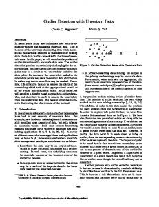
The third real data set contains 902 high-tech parts designed for consumer products and characterized by 88 electronic measures; it is available in the R package ICSOutlier (Archimbaud et al., 2016). To anonymize the data collected, the measures have been mean-centered. We do not have access to the original data, but we know that they were cleaned from univariate outliers using some preliminary standard quality control rules. No multivariate outlier detection method was applied and the parts were sold. However, two parts (denoted by R1 and R2 in what follows) among the 902 were found to be defective and returned to the manufacturer. Our objective is to check whether these two observations could have been detected before being sold, using some multivariate outlier detection method in an unsupervised way, with less than 2% of observations flagged as outliers. From Table 4, the result based on only one component (best selection) for ICS is perfect, with two outliers detected and no false detection. The results are much worse for all other methods, with too many false detections. This is especially true when considering the Mahalanobis distance with no selection of components. The results for ICS are rather mediocre when using the DA or (even worse) the PA automated selection methods which tend to select too many components. Using the scree plot, however, leads unambiguously to a more drastic selection, with three eigenvalues larger than the others. Using 24
800
600 ICSD²
100
200 0
700
700
200
400
600
800
0
ICSD2COV−1COV4(xi, k = 52) with PA: TP = 2, FP = 91
200
400
600 ICSD²
400
500
600
200
300
ICSD²
400
500
600 500 400 300 200
200
R1
100
0
0
400
600
800
0
100
100
R1
200
800
R2
R2
R1
0
600
MD2(xi) = ICSD2COV−1COV4(xi, k = p = 88): TP = 2, FP = 130
700
600
300
400
R1
0
R1
0 200
ICSD2COV−1COV4(xi, k = 14) with DA: TP = 2, FP = 39
300
400
500
600 100
200
300
ICSD²
400
500
600 500 400 ICSD²
300 200 100 0
R1
R2
ICSD²
R2
R2
R2
0
ICSD2COV−1COV4(xi, k = 3) with : TP = 2, FP = 5
700
ICSD2COV−1COV4(xi, k = 2) with : TP = 2, FP = 2
700
700
ICSD2COV−1COV4(xi, k = 1) with : TP = 2, FP = 0
0
200
400
600
800
0
200
400
600
800
Figure 5: Plots of the squared ICS distances for different numbers of invariant components selected for the HTP data set. three components leads to good performance, with five FP and all together seven detected outliers, which is less than 2% and thus acceptable. Figure 5 gives more insight on the influence of the number of selected invariant components on the detection performance and echoes Figure 1. The six scatter plots give the squared ICS distances when the number of components increases. The top-left plot corresponds to one component, which is the best possible selection. Then, the FP increases when more components are selected. The bottom-left plot corresponds to DA selection, while the bottom-middle plots correspond to PA selection. On the bottom-right plot, all 88 components are taken into account, which corresponds to the squared Mahalanobis distance, and the result is the worst. Note that for this data set, PCA performs better than the Mahalanobis distance even if the number of FP is still unacceptable. Finally, ICS is shown to be appropriate for the three data sets when using the scree plot selection method, while the performance of its competitors depends on the data set.
25
7
Conclusion and perspectives
The remarkable theoretical properties of ICS are confirmed in the context of multivariate outlier detection. Contrary to PCA, the method is scale invariant and is aimed at detecting outliers. More precisely, the present paper demonstrates the good performance of ICS, when using the scatter pair COV−COV4 and selecting the first components in a context of a small proportion of outliers. The simulation study together with the data analysis illustrates that ICS consistently detects outliers, when they are present, with a small proportion of false detections, while the success of its competitors is much less obvious. The data analysis highlights in particular the advantage of using the scree plot for selecting the number of components. For large dimensions and when outliers are contained in a small dimensional subspace, using ICS may improve greatly with respect to Mahalanobis distance as illustrated by certain theoretical properties and applications. Moreover, selecting a small number of invariant components makes outlier interpretation much easier. A perspective of the work is to consider multiple testing procedures for the choice of the cut-off for the distances as proposed by Cerioli (2010) and Cerioli and Farcomeni (2011). Another perspective is to consider the case of a large proportion of outliers. In such a context, the scatter pair choice has to be revisited together with the components choice. If outliers are contained in a small dimensional subspace, the COV − COV4 pair, even if it is not robust, may still be a good alternative given the ICS theoretical properties. However, small kurtosis values are now also of interest, and thus invariant components associated with small eigenvalues should be examined. In such a context, the recent paper by Nordhausen et al. (2016) is of particular interest.
8
Acknowledgements
The work of Klaus Nordhausen was supported by the Academy of Finland (grant 268703). The article is based upon work from COST Action (CRoNoS), supported by COST (European Cooperation in Science and Technology).
26
References Aggarwal, C. C. (2013). Outlier Analysis. Springer Publishing Company, Incorporated. Alashwali, F. and Kent, J. (2016). The use of a common location measure in the invariant coordinate selection and projection pursuit. Journal of Multivariate Analysis, 152:145– 161. Archimbaud, A., Nordhausen, K., and Ruiz-Gazen, A. (2016). ICSOutlier: Outlier Detection Using Invariant Coordinate Selection. R package version 0.1-8. Bonett, D. G. and Seier, E. (2002). A test of normality with high uniform power. Computational Statistics and Data Analysis, 40(3):435–445. Cator, E. A. and Lopuha¨a, H. P. (2012). Central limit theorem and influence function for the MCD estimators at general multivariate distributions. Bernoulli, 18(2):520–551. Caussinus, H., Hakam, S., and Ruiz-Gazen, A. (2003). Projections r´ev´elatrices contrˆol´ees: Groupements et structures diverses. Revue de Statistique Appliqu´ee, 51(1):37–58. Caussinus, H. and Ruiz, A. (1990).
Interesting projections of multidimensional data
by means of generalized principal component analyses. In Compstat, pages 121–126. Springer. Cerioli, A. (2010). Multivariate outlier detection with high-breakdown estimators. Journal of the American Statistical Association, 105(489):147–156. Cerioli, A. and Farcomeni, A. (2011). Error rates for multivariate outlier detection. Computational Statistics & Data Analysis, 55(1):544–553. Dray, S. (2008). On the number of principal components: A test of dimensionality based on measurements of similarity between matrices. Computational Statistics & Data Analysis, 52(4):2228 – 2237. Fischer, D., Berro, A., Nordhausen, K., and Ruiz-Gazen, A. (2015). REPPlab: R Interface to EPP-Lab, a Java Program for Exploratory Projection Pursuit. R package version 0.9.2.
27
Fischer, D., Berro, A., Nordhausen, K., and Ruiz-Gazen, A. (2016). REPPlab: An R package for detecting clusters and outliers using exploratory projection pursuit. Technical report, arXiv:1612.06518v1. Genz, A. and Bretz, F. (2009). Computation of Multivariate Normal and t Probabilities. Lecture Notes in Statistics. Springer-Verlag, Heidelberg. Green, C. G. (2016). CerioliOutlierDetection: Outlier Detection Using the Iterated RMCD Method of Cerioli (2010). R package version 1.1.5. Green, C. G. and Martin, R. D. (2014). An extension of a method of Hardin and Rocke, with an application to multivariate outlier detection via the IRMCD method of Cerioli. Technical report, Working Paper, 2014. Available from http://students. washington. edu/cggreen/uwstat/papers/cerioli extension. pdf. Hampel, F., Ronchetti, E., Rousseeuw, P., and Stahel, W. (1986). Robust statistics. Wiley & Sons, New York. Hubert, M., Rousseeuw, P. J., and Vanden Branden, K. (2005). ROBPCA: a new approach to robust principal component analysis. Technometrics, 47(1):64–79. Jobe, J. M. and Pokojovy, M. (2015). A cluster-based outlier detection scheme for multivariate data. Journal of the American Statistical Association, 110(512):1543–1551. Jolliffe, I. (2002). Principal component analysis. Wiley Online Library. Komsta, L. and Novomestky, F. (2015). moments: Moments, cumulants, skewness, kurtosis and related tests. R package version 0.14. Nordhausen, K., Oja, H., and Tyler, D. E. (2008). Tools for exploring multivariate data: The package ICS. Journal of Statistical Software, 28(6):1–31. Nordhausen, K., Oja, H., and Tyler, D. E. (2016). Asymptotic and bootstrap tests for subspace dimension. Technical report, arXiv:1611.04908v1. Nordhausen, K. and Tyler, D. E. (2015). A cautionary note on robust covariance plug-in methods. Biometrika, 102:573–588. 28
Penny, K. I. and Jolliffe, I. T. (1999). Multivariate outlier detection applied to multiply imputed laboratory data. Statistics in Medicine, 18(14):1879–1895. Peres-Neto, P. R., Jackson, D. A., and Somers, K. M. (2005). How many principal components? Stopping rules for determining the number of non-trivial axes revisited. Computational Statistics & Data Analysis, 49(4):974–997. R Core Team (2014). R: A Language and Environment for Statistical Computing. R Foundation for Statistical Computing, Vienna, Austria. Rousseeuw, P., Croux, C., Todorov, V., Ruckstuhl, A., Salibian-Barrera, M., Verbeke, T., Koller, M., , and M¨achler, M. (2015). robustbase: Basic Robust Statistics. 0.92-5. Rousseeuw, P. J. (1986). Multivariate estimation with high breakdown point. In Grossman, W., Pflug, G., Vincze, I., and Wertz, W., editors, Mathematical Statistics and Applications, pages 283–297. Reidel, Dordrecht. Rousseeuw, P. J. and Van Zomeren, B. C. (1990). Unmasking multivariate outliers and leverage points. Journal of the American Statistical Association, 85(411):633–639. Stahel, W. and M¨achler, M. (2013). robustX: eXperimental Functionality for Robust Statistics. R package version 1.1-4. Stahel, W. A. and M¨achler, M. (2009). Comment on “invariant co-ordinate selection”. Journal of the Royal Statistical Society B, 71(584–586). Todorov, V. and Filzmoser, P. (2009). An object-oriented framework for robust multivariate analysis. Journal of Statistical Software, 32(3):1–47. Tyler, D. E., Critchley, F., D¨ umbgen, L., and Oja, H. (2009). Invariant coordinate selection. Journal of the Royal Statistical Society: Series B (Statistical Methodology), 71(3):549– 592. Willems, G., Joe, H., and Zamar, R. (2009). Diagnosing multivariate outliers detected by robust estimators. Journal of Computational and Graphical Statistics, 18(1):73–91.
29
Yazici, B. and Yolacan, S. (2007). A comparison of various tests of normality. Journal of Statistical Computation and Simulation, 77(2):175–183.
30