Navigation and Tree Mapping in Orchards Claes L. Jaeger-Hansen1*, Hans W. Griepentrog1, Jens Christian Andersen2 1
Instrumentation & Test Engineering, Institute of Agricultural Engineering, Faculty of Agricultural Sciences University of Hohenheim, DE-70599 Stuttgart, Germany 2 Automation and Control, Department for Electrical Engineering, Technical University of Denmark, DK-2800 Kgs. Lyngby, Denmark Technical University of Denmark *E-mail:
[email protected] Abstrat In this paper an algorithm for estimating tree positions is presented. The sensors used for the algorithm is GNSS and LIDAR, and data is collected in an orchard with grapefruit trees while driving along the rows. The positions of the trees are estimated using ellipse fitting on point clouds. The average accuracy for the center point estimation is 0.2 m in the along track direction and 0.35 m in the across track direction. The goal of the tree mapping algorithm is create a database of individual trees, and be the basis for creation of a graph map that can be used for mission planning and localization for an autonomous robot. Key words: Autonomous navigation, autonomous mapping, ellipse fitting, tree detection, robotics. 1. Introduction In this paper an algorithm for estimating tree positions is presented. Based on the recorded data from a grapefruit orchard in Turkey at Cukurova University the algorithm will be derived and tested. More and more machines and robots are today relying on autonomous navigation. In orchards autonomous navigation can be a difficult task. The problem that is most often encountered is the reliability of the Global Navigation Satellite System (GNSS) receivers. Orchards come very close to being structured environments, which means that robots and autonomous vehicles have various possibilities for navigation. Already several solutions on how to navigate in orchards without a priory knowledge exists, (Barawid et al. 2007, Linker & Blass 2008 and Christensen 2011). But none of them handles the problems with headland turning efficiently. MobotWare, a software framework for controlling robots (Beck et al. 2010), has solved this problem using a combination localization of LIDAR, INS and a map of the orchard, as described in Andersen et al. 2010. The problem using MobotWare is that you need a graph map of the orchard to be able to create missions for the robot, and to do localizations without GNSS. Several researches are and have been working on solutions where the robot does not have to rely on the GNSS receivers for navigation. Instead the navigation is relying on other sensors like Inertial Measurement Unit (IMU) and laser scanner (LIDAR). The system described in Andersen et al. 2010 can perform navigation and localization in orchards based on an a priory map (graph map based on nodes and edges) and a LIDAR. A map describing the orchard has to be created, in order to define and create mission for autonomous vehicles. The goal is to create such a map automatically based on laser scanner data and GNSS position data recorded in the orchard. The data needed to create such a map is the position of the trees and an approximate value for the tree foliage radius. The foliage radius is needed for localization and to limit the available manoeuvre space for the robot.
Along with the graph map creation, the position of each tree must be calculated and exported, so it can be used in other applications like GIS and farm managing tools. In the 3DMosaic project1 the position of each tree is needed for a GIS system. Instead of measuring each position by hand the goal is to calculate an estimated position of each tree. The algorithm described in this paper is trying to use as simple tools as possible to calculate the positions and foliage radius for the trees. The algorithm is used as a proof of concept, to determine if it is possible to calculate an estimated position of the trees based on LIDAR and GNSS data only. 2. Mapping At the moment there are two ways to create a graph map. The first way is to go into the orchard with a GNSS receiver and manually measure the points which are needed to create the map. The second way is to use Google Earth to get the same data. In both cases the map has to be created manually afterwards. It is one of the goal to automate this process via a mapping algorithm. Currently the algorithm consists of four steps. 1. Combine all laser scanner data to show a row in the orchard. 2. Tree detection in the combined laser scanner data. 3. Estimate the position of each tree using ellipse fitting. 4. Export the tree position map. At this time the algorithm is not supposed to be running in real-time. It is meant for post process calculation. It needs all the laser scan data for an entire row in order to work correctly. If it is to be implemented in real-time the ellipse fitting needs to be changed, and the modified – less accurate – version could be used while driving to identify the trees and localize the robot, once the map is established. 2.1 Data collection The data used for this paper has been recorded from a Sick LSM-111 laser scanner and Trimble AgGPS-542 RTK-GNSS receiver. The sensors where mounted on a tractor (see figure 1). This setup was driven manually through each row of the orchard while recording the data. 2.2 Tree detection Figure 2 shows three different examples of what grapefruit trees looks like, when seen by a laser scanner. The noise in figure 2a is ground detection caused by terrain curvature, but it is included to test the ellipse fitting methods. In figure 2b an almost perfect tree is shown. With a point cloud like this the ellipse fitting algorithm should have no problem. In figure 2c a tree where there is a hole in the canopy closest to the track. The hole is big enough to confuse some algorithms, and maybe pose as a problem when trying to detect tree borders. As the LIDAR is forward looking, the highest amount of detections is on the front side of the trees, as can be seen on the figures. The noise from figure 2a may vary, but nevertheless these three types of point clouds are the expected shapes of grapefruit trees in the data. Based on the different detection shapes of the trees, shown in figure 2, the most effective way to detect a tree could be to find the borders of the tree and run the point cloud of each tree through an ellipse fitting algorithm.
1
http://www.atb-potsdam.de/3d-mosaic/
FIGURE 1 The tractor and the sensors used for data collection
FIGURE 2 Example of three single trees. The tractor passes the trees parallel with the vertical axis at the zero position on the horizontal axis. a) Tree cluttered with ground detection noise, b) without noise and c) without noise but with hole in the foliage closest to the track. Axes are in meters. The density of LIDAR hits is largest on front and back of the tree, relative to the track direction. This means there should be a local minimum of LIDAR hits between the trees, and maybe also in the middle of the canopy closest to the track, where there is a hole. It should then be possible to detect the borders between the tree by creating and analyzing a histogram showing the count of LIDAR hits for each meter in the tree row. 2.3 Histogram Analysis The histogram G in figure 3 is crated based on the count of measurement point’s yn within each meter at the position xn along the track at a distance across the track from 1 m to 8 m. The vertical red lines show the tree borders that were selected manually, the vertical blue lines show the borders calculated from the histogram. The borders of the trees are found in the histogram where a minimum occurs. To determine which minima to use as borders a priory knowledge is necessary. The trees are planted with a separation of about 8 m, so therefore the distance between each minimum has to be larger than 7 m. If the distance between each minimum is smaller, it might detect a hole in the middle of the tree as seen in figure 2c. Equation 1 describes how to locate each minimum. G is a vector that contains the (xn,yn) points of the histogram in figure 3. M is a vector containing all tree separation minima xm, starting from x0=0 m. ∈ |
∧
7
(1)
A comparison between the borders created manually and the borders calculated from the histogram, shown in table 1, shows this method is valid. There are several places where there is a difference of one meter between the manually created borders and the calculated
borders. Testing has shown that the difference between the centers of the resulting ellipses can be neglected.
FIGURE 3 Histogram showing the count of LIDAR hits for each meter. TABLE 1Tree border comparison along a 200m long row with 23 grape fruit trees Manual 0 9 17 26 35 43 52 61 69 78 86 95 Histogram 0 9 17 26 35 44 52 60 69 78 86 95 Manual 104 112 121 129 138 147 156 163 171 181 190 Histogram 103 112 121 129 138 147 155 164 172 180 190
198 198
2.4 Ellipse fitting algorithms Several ellipse fitting methods were considered, Taubin ellipse fitting (Taubin 1991), Direct Least Square Ellipse fitting (Fitzgibbon et al.,1996), Ransac, Hough transform, Hyper Accurate Ellipse Fitting. The methods selected for testing are Taubin and Direct Least Square Ellipse Fitting (DLS). The two methods were tested on the tree from figure 2a, with significant noise from ground detection. Figure 4 shows the result of the test, both methods are robust, and can handle the noise in this case. The black ellipse is the Taubin ellipse and the blue is the DLS. The two methods react differently on the noise as can be seen in table 2. But the center point of the ellipses is within 0.1 m of each other. Table 2 shows the parameters for the two ellipses in figure 4. The two radii in each ellipse is different, but both are reasonable representative for the tree. TABLE 2 Ellipse parameters from the ellipses in figure 4 Taubin Direct Least Square Fit R1
1.5233
R1
2.9311
R2
3.7717
R2
1.6843
X
-3.8583
X
-3.7635
Y
4.9065
Y
4.8383
The most interesting part is the center point of the ellipses. They are within 0.1 m in both the vertical and horizontal direction. The average radius is 2.65 m (Taubin) and 2.3 m (DLS), this radius is a bit exaggerated, as the data is not corrected for roll and tilt of the GNSS antenna (see figure 1). Both methods are robust enough to handle noise and both methods can be used in to estimate both the tree position and the foliage radius.
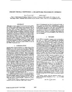
FIGURE 4 Ellipse fitting test. The black ellipse is Taubin, the blue is Direct Least Square Fitting. The comparison in figure 4 shows that DLS fitting is better for estimating the foliage radius than Taubin. The desired accuracy of the estimated center point is 1 m in across track direction, and 0.5 m in along track direction. Figure 5b shows two trees and the ellipses derived from DLS. The error in the uppermost tree is the largest error in the data set. The Taubin method give no solution for the estimation of this tree. Because DLS is better for estimating the foliage radius and it gives a solution for all trees, the DLS method is selected to estimate the tree positions.
FIGURE 5 Estimated ellipses and borders in the laser scanner data.
3. Result When applying the borders calculated from the histogram and using DLS on each point cloud, the estimated position of each tree in one row can be seen in figure 5a. Some of the estimated ellipses in figure 5a are estimated with a rather poor accuracy. An example is shown in figure 5b, where the uppermost ellipse has an across track error of approximately 1 m. The average accuracy for the center point estimation is 0.2 m in the along track direction and 0.35 m in the across track direction. The accuracy is based on a manual estimation from the trees where the tree trunk is clearly visible in the dataset. 4. Conclusion Using the algorithm described it is possible to calculate a trees position, based on the center points for the estimated ellipses. It is possible to export the positions in a format which can be imported in GIS systems. It is also possible to run the coordinates through a parser that can generate an graph map of the orchard, which can be used for mission generation and execution. The accuracy of the algorithm is at this point high enough to create a graph. But depending on the application, it may not be high enough for GIS systems. Acknowledgement We would like to thank the institutions that made the project 3D-Mosaic possible. Bundesanstalt für Landwirtschaft und Ernährung (BLE) who are funding our participation in this EU-project through ICT-AGRI and ERA-Net. Reference list Andersen, J. C., Ravn, O. , Andersen, N. (2010). Autonomous rule-based robot navigation in orchards, International Federation of Automatic Control, 2010. Aschoff, T. & Spiecker, H. (2004). Algorithms for the Automatic Detection of Trees in LaserScanner Data, ISPRS Volume XXXVI-8/W2, 2004. . Barawid, O., Mizushima, A., Ishii, K., & Noguchi, N. (2007). Development of an autonomous navigation system using a two-dimensional laser scanner in an orchard application, Biosystems Engineering (2007) 96 (2), 139–149. . Chernov, N. (2009). http://www.mathworks.com/matlabcentral/fileexchange/22683-ellipse-fittaubin-method. Christensen, M. (2011). Localization in orchards using Extended Kalman Filter for sensorfusion, University of Southern Denmark (SDU), Faculty of Engineering, Master Thesis. . Fitzgibbon, A. W., Pilu, M., Fisher, R. B. (1996). Direct Least Squares Fitting of Ellipses, Proceedings of ICPR - IEEE 1996, 253-257. . Linker, R., Blass, T. (2008). Path-planning algorithm for vehicles operating in orchards, Biosystems Engineering 101(2008) 152 – 160. . Pilu, M (1996). demo.html .
http://homepages.inf.ed.ac.uk/rbf/CVonline/LOCAL_COPIES/PILU1/
Taubin, G. (1991). Estimation of planar curves, surfaces, and nonplanar space curves defined by implicit equations with applications to edge and range image segmentation, IEEE Transactions on Pattern Analysis and Machine Intelligence — 1991, Volume 13, Issue 11, pp. 1115-1138. . Beck, A. B., Andersen, N. A., Andersen, J. C., Ravn, O. (2010). Mobotware – A Plug-in Based Framework For Mobile Robots. IAV 2010. International Federation of Automatic Control, 2010.