ments, CSEM systems were applied to groundwater prospecting in arid or hard- rock environments. ... Standard physics textbooks such as Wangsness (1986).
NEAR-SURFACE CONTROLLED-SOURCE ELECTROMAGNETIC INDUCTION: BACKGROUND AND RECENT ADVANCES MARK E. EVERETT Dept. of Geology and Geophysics, Texas A&M University College Station TX 77843 U.S.A. MAX A. MEJU Dept. of Environmental Science, Lancaster University Lancaster LA1 4YQ, U.K. 6.1. Introduction The controlled-source electromagnetic (CSEM) induction method is emerging as a leading geophysical technique in hydrogeological studies. However, the technique is quite often misunderstood compared to other common techniques of applied geophysics: namely, seismic reflection and refraction, magnetics, gravity, and ground-penetrating radar (GPR). In this chapter we review the fundamental physical principles behind the CSEM prospecting technique, with emphasis on near-surface applications, and present some recent advances in this field that have been made by the authors. CSEM methods are defined here to be those in which the experimenter has knowledge of and control over the electromagnetic field transmitted into the ground and hence excludes magnetotellurics, related natural-source methods, and the various uncontrolled–source methods involving, for example, radio transmissions. CSEM methods for investigating subsurface geology began in earnest in the 1950’s and 1960’s with the advent of airborne systems mainly for mining applications. Later, with the development of portable and inexpensive ground-based instruments, CSEM systems were applied to groundwater prospecting in arid or hardrock environments. Due to the upsurge in interest in environmental applications in the past one or two decades, the CSEM method is currently experiencing a rapid growth in use by hydrogeologists, civil and geotechnical engineers, engineering geologists, and others not trained specifically in the technique. The CSEM method is sensitive to electrical conductivity averaged over the volume of ground in which induced electric currents are caused to flow. Amongst the surface-based geophysical methods that sense bulk electrical properties of the ground, CSEM offers deeper penetration capability than GPR techniques and greater resolving power than DC resistivity methods. The CSEM method performs well in conductive soils or high radar reflectivity zones where GPR often encounters difficulties. The CSEM method also performs well in highly resistive terrains where establishing good electrode contact with the ground, as required for most DC methods, often is problematic.
CSEM techniques play an important role in hydrogeophysical investigations since the sensed physical property, electrical conductivity, is linked petrophysically to hydrological variables of interest such as moisture content, hydraulic conductivity, porosity, and so forth. This chapter focuses on the relationship between CSEM measurements and spatially-averaged subsurface electrical conductivity; it does not address the correspondence between electrical conductivity and hydrological variables. Information on this important topic can be found in Chapter 3. CSEM case histories relevant to hydrogeophysics are found in Chapter 13. The CSEM should be attractive to hydrogeologists also because it is simple to operate in the field with the current generation of inexpensive commercial instruments. A variety of data processing options are available, ranging from construction of apparent conductivity curves based on simple asymptotic formulas for rapid subsurface evaluation all the way to 1-D, 2-D and advanced 3-D forward modeling and inversion for more detailed analyses. Previous reviews of CSEM studies for near-surface applications have been carried out by Nobes (1996) and Tezkan (1999). Tutorial articles specifically concerned with the CSEM method are by McNeill (1980a,b) and West and Macnae (1991) while theoretical treatments are available in the books by Grant and West (1965), Ward and Hohmann (1987), Wait (1982) and Zhdanov and Keller (1994). Senior or graduate level exploration textbooks such as Telford et al. (1990), Sharma (1997) and Kearey et al. (2002) provide a brief overview of the CSEM method along with case studies. Standard physics textbooks such as Wangsness (1986) and Jackson (1998) are useful for review of the underlying laws of classical electromagnetism, however these texts emphasize wave propagation in dielectric media over electromagnetic induction in conducting media. The older books by Jones (1964), Stratton (1941) and Smythe (1967) treat induction in more detail and are recommended for advanced study. In order to use CSEM data for hydrogeological applications, it is important for potential practitioners to understand the basic physics of the technique and how factors such as noise, scaling, and inversion impact the interpretation. This chapter is organized as follows. After an overview of the CSEM method, the basic physics behind frequency and time-domain CSEM prospecting systems is discussed, followed by a discussion on CSEM applications to hydrogeophysical problems and a brief account of 3-D forward modeling. Then, inversion of CSEM data is treated. The paper concludes with an outlook and discussion section. The emphasis in this paper is on inductively-coupled loop-loop CSEM systems, although other configurations including those that employ a directly-coupled source will be discussed. Loop-loop systems are chosen to simplify the discussion and because they are easy to use in the field and widely employed in hydrogeophysical applications.
6.2. CSEM Overview The CSEM method of geophysical prospecting is founded on Maxwell’s equations that govern electromagnetic phenomena. Combining Ohm, Ampere and Faraday laws (Wangsness, 1986; Jackson, 1998) results in the damped wave equation ∇2 B − µ 0 σ
∂B ∂2B − µ0 � 2 = µ0 ∇ × JS , ∂t ∂t
(6.1)
where B is magnetic field, µ0 is magnetic permeability, σ is electrical conductivity, � is dielectric permittivity, JS is the source current distribution, and t is time. In the CSEM method for most hydrogeophysical applications, the earth is generally considered to be non-magnetic, such that µ0 =4π ×10−7 H/m, the magnetic permeability of free space. This assumption can break down if highly magnetic volcanic soils or ferrous metal objects are encountered, in which case the ground or target magnetic permeability influences the CSEM response and should be taken into account. The electrical conductivity of most near-surface geological materials lies in the range σ=0.0001-0.1 S/m (Palacky, 1987). The third term on the left hand side of equation (6.1) is the energy storage term describing wave propagation (Powers, 1997). The second term on the left hand side of equation (6.1) is the energy dissipation term describing electromagnetic diffusion. The CSEM method, which is the topic of our consideration, operates at low frequencies (∼100 Hz to 1 MHz), or alternatively, slow (∼1 µs to 10 ms) disturbances of the source currents. In this case, |σ∂B/∂t| is larger by several orders of magnitude than |�∂ 2 B/∂t2 |, so that the wave propagation term is safely ignored and dielectric permittivity � plays no further role in the discussion. The result is that CSEM is a purely diffusive phenomenon. If the electrical conductivity is low enough and the frequency high enough that σ∼ �ω, the electromagnetic response of the earth is properly described by equation (6.1) with all terms kept.
6.3. Basic Physics, Time Domain A physical understanding of CSEM responses can be obtained by recognizing that the induction process is equivalent to the diffusion of an image of the transmitter (TX) loop into a conducting medium. The similarity of the equations governing electromagnetic induction and hydrodynamic vortex motion, first noticed by Helmholtz, leads directly to the association of the image current with a smoke ring (Lamb, 1945; p.210). The latter is not “blown,” as commonly thought, but instead moves by self-induction with a velocity that is generated by the smoke ring’s own vorticity and described by the familiar Biot-Savart law (Arms and Hama, 1965). An electromagnetic smoke ring dissipates in a conducting medium much as the strength of a hydrodynamic eddy is attenuated by the viscosity of its host fluid (Taylor, 1958; pp.96-101). The medium property that dissipates the electromagnetic smoke ring is electrical conductivity.
An inductively-coupled time domain CSEM (TDEM) system is shown in Figure 6.1a. A typical TX current waveform I(t) is a slow rise to a steady-on value I 0 followed by a rapid shut-off, as exemplified by the linear ramp in Figure 6.1b (top). Passing a disturbance through the TX loop generates a primary magnetic field that is in-phase with, or proportional to, the TX current. According to Faraday’s law of induction, an impulsive electromagnetic force (emf) that scales with the time rate of change of the primary magnetic field is also generated. The emf drives electromagnetic eddy currents in the conductive earth, notably in this case during the ramp-off interval, as shown in Fig.6.1b (middle). After the ramp is terminated, the emf vanishes and the eddy currents start to decay via Ohmic dissipation of heat. A weak, secondary magnetic field is produced in proportion to the waning strength of the eddy currents. The receiver (RX) coil voltage measures the time rate of change of the decaying secondary magnetic field, Fig. 6.1b (bottom). In many TDEM systems, RX voltage measurements are made during the TX off-time when the primary field is absent. The off-time advantage is that the relatively weak secondary signal is not swamped by the much stronger primary signal. A good tutorial article on TDEM is by Nabighian and Macnae (1991.)
(a)
(b) V(t)~dBz/dt
TX current, I(t) I0 steady ON fast ramp-off (~ms)
slow rise (~ms)
I(t)= RX
time, t
induced emf, V(t)
TX
rectangular impulse (ms) time, t
conductivity, σ(r)
eddy currents "smoke-ring diffusion"
secondary magnetic field, H(t)
RX time gates
123 4
5 time, t
slow decay (~ms)
Fig. 6.1. (a) TX loop lying on the surface of an isotropic uniform halfspace of electrical conductivity, σ . A disturbance I(t) in the source current immediately generates an electromagnetic eddy current in the ground just beneath the TX loop. A RX coil measures the induced voltage V (t), which is a measure of the timederivative of the magnetic flux generated by the diffusing eddy current. (b) Typical TX current waveform I(t) with slow rise time and fast ramp-off; induced emf V (t), proportional to the time rate of change of the primary magnetic field; decaying secondary magnetic field H(t) due to the dissipation of currents induced in the ground. During the ramp-off, the induced current assumes the shape of the horizontal projection of the TX loop onto the surface of the conducting ground. The sense of the circulating induced currents is such that the secondary magnetic field they create tends to maintain the total magnetic field at its original steady-on value
prior to the TX ramp-off. In this case, therefore, the induced currents flow in the same direction as the TX current, i.e. opposing the TX current decrease that served as the emf source. The image current then diffuses downward and outward while diminishing in amplitude. In TDEM offset-loop soundings, the TX and RX loops are separated by some distance L. As indicated in Figure 6.2a, at a fixed instant in time t, the vertical magnetic field Hz (L) due to the underground circuit exhibits a sign change from positive to negative as distance L increases. Alternatively, the vertical magnetic field Hz (t) changes sign from positive to negative as the filament passes beneath a fixed measurement location. The “normal moveout” of the sign reversal with increasing TX-RX separation distance is shown in Figure 6.2b, Field examples from Utah and Texas showing sign reversal in the TDEM offset-loop response are shown in Figure 6.3.
(a)
(b) RX coils
σ=0.1 S/m TEM47 ramp-off voltage [mV]
flux < 0 flux = 0 flux > 0
TX
smoke-ring diffusion
L=10 m
30 60
100
TEM47 time gate
Fig. 6.2. (a) The electromagnetic smoke ring may be viewed as a system of equivalent current filaments diffusing downward and outward from the TX loop (Nabighian, 1979). The equivalent filament concept can be used to understand the spatiotemporal behavior of the voltage induced in a horizontal RX coil. The figure shows that, at a fixed instant in time t, the flux–proportional vertical magnetic field Hz (x) due to the underground circuit exhibits a sign change from positive to negative as distance x increases from the TX loop. Similarly, at a fixed location in space, the vertical magnetic field Hz (t) also changes sign from positive to negative as the filament passes beneath a RX coil. The apparent conductivity of the ground is determined by analyzing the times at which the sign reversals occur in the various RX coils. (b) Transient decays for a loop-loop CSEM system (Geonics PROTEM47) over a uniform halfspace. The time of the sign reversal increases with TX-RX separation distance L, in meters. Dashed line: negative voltage; solid line: positive voltage.
A mathematical treatment of the electromagnetic smoke ring phenomenon ap-
pears in Nabighian (1979). Hoversten and Morrison (1982) and Reid and Macnae (1998) have further explored smoke-ring diffusion into a layered conducting earth. These papers provide physical insight which can greatly assist hydrogeophysicists to understand the TDEM response in idealized situations. The description of a directly-coupled TDEM system is similar to the inductively-coupled case, but requires additional physics due to the presence of ground-contacting electrodes.
(a)
(b)
1000 σ=0.016 S/m
100
h=33 m
σ=1.0 S/m
10
1
Paria, UT
100 L=41.1 m
conductivity, S/m
TEM47 ramp-off voltage [mV]
L=57.5 m
TEM47 ramp-off voltage [mV]
1000 .13 .12 .11
σ(z)
.10 .09 10 20 30 40 50 60
depth, m
10
Brazos, TX 1
6 10 20 30 60 time after ramp-off initiation [ms]
TEM47 time gate
Fig. 6.3. (a) A transient sounding using the Geonics PROTEM47 loop-loop configuration (TX loop radius, 2 m) observed atop an eolian Page Sandstone outcrop near Paria Campground, UT. The response of the 2-layer model in the insert is also shown. (b) A similar PROTEM47 sounding observed over Brazos, TX clay-rich floodplain alluvium, after Sananikone (1998). The response of the smooth model σ(z) in the insert is also shown. The low conductivity at depths ∼9-12 m owes to a sand and gravel aquifer overlying basement shale.
6.3.1 TDEM APPARENT CONDUCTIVITY The conductivity of the ground can be estimated from TDEM offset-loop sounding responses by analyzing the times at which sign reversals occur in the various RX coils. It is sometimes convenient, on the other hand, to transform TDEM sounding data into an apparent conductivity curve. Apparent conductivity is defined (Spies and Friscknecht, 1991) as the conductivity of the uniform halfspace that would generate the observed response at each discrete measurement time after the TX ramp-off. Caution is required however since for some electrical conductivity structures at certain time gates the apparent conductivity can be non-existent or multi-valued. Examples of apparent conductivity curves for two synthetic and one actual field
TDEM offset-loop response are given in Figure 6.4. The synthetic responses were generated by forward modeling of transient EM induction in a two-layer conductivity structure. The apparent conductivity at each time gate was calculated by matching the response at that time gate to the synthetic response of a uniform half-space. The trend of an apparent conductivity curve with increasing time is roughly indicative of the trend of the subsurface electrical conductivity with increasing depth, assuming that a layered structure is a good approximation to the electrical conductivity of the underlying geological formations.
(b) apparent conductivity [S/m]
TEM47 ramp-off voltage [mV]
(a)
time gate
time gate
Fig. 6.4. (a) Geonics PROTEM47 responses. Symbols represent the Paria, UT response shown in the previous figure. The heavy line is the synthetic response of a resistive layer (0.02 S/m, 10 m thick) overlying a conductive halfspace (0.2 S/m). The lighter dashed/solid line shows the negative/positive portions of the synthetic response of a conductive layer (0.2 S/m, 10 m thick) overlying a resistive halfspace (0.02 S/m.) (b) The corresponding apparent conductivity curves, showing trends with increasing time that reflect trends of electrical conductivity with increasing depth. The gap in the apparent conductivity curve for the conductor-over-resistor model indicates that no uniform conductor can be found with a response that exactly matches the two-layer response for PROTEM47 time gates 5-8. Various asymptotic formulas for apparent conductivity that are valid at either early or late times after TX ramp-off have been developed (Spies and Frischknecht, 1991.) They yield estimates of shallow (z�L) and deep (z�L) electrical conductivity, respectively. Other TDEM sounding configurations also may be analyzed using apparent conductivity. In the popular central loop configuration, a RX coil is placed in the center of the TX loop. No sign reversal occurs. In this type of TDEM sounding, the shape and strength of the decaying transient are used to determine apparent conductivity, either by exact forward modeling or using asymptotic formulas. In the coincident loop method, the TX and RX coils are col-
located. Apparent conductivity in this case is often computed using the method of Spies and Raiche (1980).
6.4. Basic Physics, Frequency Domain In the frequency domain methods (FDEM), the TX current oscillates at a given angular frequency, ω. The emf, being proportional to the rate of change of primary magnetic field, is out of phase with the TX current. The emf drives eddy currents in the conductive earth. The secondary magnetic field due to the induction of eddy currents contains both in–phase and out–of–phase (quadrature) components owing to the complex impedance of the ground. Excellent, rigorous treatments of the frequency domain theory of CSEM induction may be found in Grant and West (1965), Wait (1982), and Zhdanov and Keller (1994). In hydrogeophysical applications, FDEM is typically applied at sufficiently low frequencies that the response is equivalent to that of a system of uncoupled electric circuits containing only passive inductive and resistive elements. This approximation is equivalent to the low-induction-number (LIN) principle upon which terrain conductivity meters such as the Geonics EM31 and EM34 instruments operate (McNeill, 1980b). The approximation is good provided the frequency is low enough that the effective penetration depth, or skin depth δ given by p δ = 2/µ0 σω, (6.2) is much greater than the TX-RX intercoil spacing L.
At LIN frequencies, each layer in the ground can be modeled to first-order as a separate wire loop. The LIN principle is equivalent to the Doll approximation (Doll, 1949) which has long formed the conceptual basis for analysis of induction logs in the petroleum industry, and assumes that the mutual inductance between each pair of underground loops is negligible. The response at the RX loop, in such case, is the sum of the primary magnetic flux from the TX loop plus the sum of the secondary magnetic fluxes generated by the induced currents flowing in the circuits. A representation of the LIN circuit approximation for a 2-layer earth is shown in Figure 6.5a. The mutual inductance M12 defined as the magnetic flux through circuit 1 caused by a unit current flow in circuit 2 (Wangsness, 1986, p.312) is assumed to be negligibly small. The primary magnetic field Hp (ω) due to timeharmonic excitation of the TX loop at frequency ω generates an out-of-phase, or quadrature, emf in each of the underground circuits, according to Faraday’s Law. The emf’s drive induced currents in the circuits. These currents each generate a secondary magnetic field that is flux-linked to the RX loop. The total secondary field Hs (ω), along with the primary magnetic field Hp (ω), is measured by the RX loop. The primary field is known precisely since the TX and RX loops are under control of the experimenter.
(a)
(b) TX
RX
R1
M12
L1
R2
L2
Fig. 6.5. (a) A conceptual view of low-frequency CSEM induction as the interaction between the time-harmonic primary magnetic flux from a TX loop and underground circuits (resistance Ri , self-inductance Li ) with vanishing mutual inductance, M12 =0. The secondary flux due to the induced currents flowing in the underground circuits is measured at the RX loop. After McNeill (1980b). (b) Field example from a gravel deposit near La Grange TX. illustrating the utility of EM34 σapp (x) profiles for lateral reconnaissance. The sharp increase in σapp near station 125 marks an abrupt transition from electrically resistive gravel of economic value to conductive, interbedded sands and clays.
The ratio of secondary to primary magnetic fields over a homogeneous halfspace, in the Doll or LIN approximation (δ�L), is derived by McNeill (1980b) as Hs/Hp = iωµ0 L2 /4,
(6.3)
which can be re-arranged to define the apparent conductivity σapp of the ground as Q
σapp = 4 [Hs/Hp] /ωµ0 L2 , where the notation [ ]
Q
(6.4)
refers to quadrature component.
The Geonics EM34 instrument can be operated in either vertical or horizontal dipole modes. In vertical dipole mode, the TX and RX coils are coplanar horizontal. As illustrated by curves in McNeill (1980b), the operating frequency (10-100 kHz range) is such that the apparent conductivity σapp in this orientation is sensitive to electrical conductivity variations in the depth range 0.3L2L.
Interpretation of FDEM responses is typically performed by analyzing the behavior of apparent conductivity σapp (x) as a function of the TX-RX midpoint position x along a profile while the TX-RX intercoil spacing L and operating frequency ω are kept fixed. Terrain conductivity meters such as EM34 provide information to a few tens of meters in depth but with limited resolving power since they operate at just a single frequency. The GEM3 system from Geophex, Ltd. operates at multiple frequencies spanning 2-3 decades in the range 100 Hz-50 kHz but depth resolution remains modest since earth’s FDEM response is a slowly varying function of frequency in this band (Huang and Won, 2003).
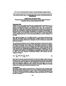
Fig. 6.6. EM34 mapping of a buried near-surface fault in a Cambrian sandstone aquifer near Mason TX, after Gorman (1998). The electrically resistive, coarsegrained Lower Hickory unit is juxtaposed to the more conductive, fine-grained Middle Hickory unit. The inferred fault location is shown by the dashed line at station 100. The various symbols indicate different TX-RX separations: L=10 m, solid dots; L=20 m, squares; L=40 m, stars. The station interval is 5.0 m.
Terrain conductivity meters are much better suited for rapid, non-invasive reconnaissance mapping of lateral changes in near-surface electrical conductivity. Figure 6.5b illustrates the use of EM34 terrain conductivity mapping to determine the lateral extent of a subsurface economic gravel deposit. This example demonstrates the use of the FDEM technique to map paleochannels comprised of coarse sediments. Roughly speaking, fine-grained material with abundant clay is conductive
while clean, coarse-grained sediment is resistive. In Figure 6.6, the EM34 method at three different frequencies is used to map faults and stratigraphic contacts in a consolidated sandstone aquifer. The faults and contacts act as barriers and conduits compartmentalizing groundwater flow in the aquifer. In both EM34 field examples, the lateral contrasts in apparent electrical conductivity are due to sharp lateral contrasts in texture.
6.5. CSEM Hydrogeophysics 6.5.1 HYDROGEOPHYSICAL TARGETS The CSEM method was originally developed and continues to be refined for natural resource prospecting and reserve evaluation applications (Meju, 2002) such as mining geophysics in which conductive ore bodies form excellent, compact targets within resistive host crystalline rocks. The CSEM method is also able to identify conductive fracture zones in crystalline bedrock aquifers for groundwater prospecting applications (Meju et al., 2001). In FDEM applications, fracture zones are typically identified by the presence of anomalously high apparent conductivity readings along a measurement profile. Typical length scales in mining and groundwater problems range from tens of meters to tens of kilometers. As Figure 6.7a dramatically illustrates, a generic hydrogeophysical site characterization problem is very difficult. The subsurface geology may contain quasilocalized features such as the weathered mantle, bedrock, bedding planes, faults, joints, fracture zones in addition to continuously distributed textural and compositional variations. In fact, due to the evident multiscale complexity, a geological medium is often viewed as a discrete hierarchy (Vogel et al., 2002), in which different length scales possess different patterns of spatial variability and correlation; or a fractal (Mandelbrot, 1988), in which each length scale possesses a similar pattern of spatial variability and correlation. The spatiotemporal CSEM response of a discrete hierarchial or fractal medium is likely to be very complicated, characterized by a broadband, power-law spatial wavenumber spectrum (Everett and Weiss, 2002). It is the difficult task of the EM hydrogeophysicist to interpret such CSEM responses in terms of the subsurface geology with its attendant spatial complexity. The presence of man-made conductors in the subsurface adds to the difficulty. However, man-made objects tend to be geometrically regular, more or less, rather than hierarchial or fractal. This offers the possibility that such objects may be detected by their band-limited wavenumber spectrum, or localized by spatial/wavenumber analysis using, for example, the continuous wavelet transform (Benavides and Everett, 2003). 6.5.2 THE SCALE EFFECT Much has been written in the hydrological literature on the effect of measurement
scale on hydraulic conductivity (Neuman, 1994; Winter and Tartakovsky, 2001). For example, due to the increased likelihood of a hydraulic test being influenced by a connected pathway from injection to monitoring well, hydraulic conductivity estimates tend to increase with increasing measurement scale, as shown in Figure 6.7b. Basin-scale hydraulic conductivity estimates are often 1-2 orders of magnitude higher than aquifer pump-test determinations, which in turn are larger than laboratory measurements on core samples of the same aquifer material. Hydraulic and electric conductivity are both transport properties of geological media that depend on geometric parameters at many length scales such as the connectivity of fracture networks and the tortuous microstructure of the pore space (see Chapter 5). Thus, electrical conductivity should exhibit a similar scale effect but field-based studies are rare (Purvance and Andricevic, 2000).
(b) TX
RX
hydraulic conductivity, K [m/s]
(a)
basin
10-2
karst 10-4 borehole
fractures 10-6 laboratory
porosity
10-1 100 101 102 103 104 scale of measurement [m]
Fig. 6.7. (a) A challenge for CSEM hydrogeophysics: sinkhole associated with coal mining subsidence at Malakoff, TX. (b) The dependence of hydraulic conductivity on measurement scale, after Person et al. (1996). 6.5.3 INCOHERENT AND COHERENT NOISE IN CSEM DATA The CSEM method measures electric or magnetic fields. For accurate and reliable interpretation of the responses in terms of subsurface geology it is important to recognize the various sources of electromagnetic noise that may be present in CSEM responses. Foremost, it is essential to differentiate between coherent and incoherent noise. Incoherent noise is temporally uncorrelated with the transmitted source current. In Figure 6.8, the main sources of environmental incoherent noise are shown. In the frequency range of interest for hydrogeophysical studies, 100 Hz-1 MHz, the predominant environmental noise sources (sferics) are caused by impulsive lightning discharges whose EM radiation can propagate over thousands of kilometers within the Earth-ionosphere waveguide. The labels TEM and TM refer to different
magnetic field, nT/(Hz)1/2
waveguide modes of propagation (Wait, 1962) while the shape of the background continuum within the sferics band is determined by the cutoff frequencies of the various modes (Porrat et al., 2001). The lower frequency continuum below 1 Hz is due to large-scale geomagnetic pulsations that arise in response to the solar wind interaction with Earth’s magnetosphere.
1
GEOMAGNETIC
SFERICS POWER LINE
10-2
10-4
VLF TEM
10-2
1
102 frequency, Hz
TM 104
Fig. 6.8. Electromagnetic noise spectrum in the frequency range of interest to CSEM hydrogeophysical investigations, after Palacky and West (1991). The spectral lines superimposed on the background continuum in Fig.6.8 are due to 50/60 Hz power line harmonics and radio signals from very low frequency (VLF) transmitters used primarily for military communication. Newman et al. (2003) describes the application of a method that utilizes VLF radio signals for hydrogeophysical investigations of the near-surface, but for the most part these transmissions are a source of noise. Other types of incoherent noise include motional noise induced in the RX coil and electronic and thermal noise in the RX amplifiers. Incoherent noise in TDEM data generally is treated by filtering and stacking the received signal. Sferics appear as irregularly spaced, high amplitude spikes of brief (ms) duration in RX voltage time series. Robust statistical methods are required for efficient sferics reduction (Buselli and Cameron, 1996). While incoherent noise sources pose a modest challenge to accurate CSEM data interpretation, much of the data processing is performed internal to the commercial instrument and hence is transparent to the user. Coherent noise however is much more problematic. Such noise is temporally correlated with the transmitted source current and can include transmitter or receiver loop misalignment or instrumental drift. These effects are reduced by careful experimental and data processing procedures. Other sources of coherent noise are currents induced in conductive structures that are not the primary target of the hydrogeophysical investigation. The two major classifications are geological and cultural noise.
Geological noise (Everett and Weiss, 2002) is defined as the electromagnetic field that is generated by induced currents flowing in fine-scale geological heterogeneities that are too small, numerous or complicated to be described in detail and hence accounted for in numerical simulations (see later section on 3-D forward modeling.) Cultural noise (Qian and Boerner, 1995) is defined as the electromagnetic field generated by currents induced in man-made conductors such as pipelines, buried tanks, steel fences, buried metal drums or other objects. These conductors must be included in numerical simulations, if possible, so that their distorting effects on the CSEM response can be properly evaluated. As an example, the effect on measured TDEM responses of a small steel sphere buried in alluvium soil is shown in Figure 6.9. Geological and cultural noise cannot be filtered or stacked out of CSEM data because of the mutual induction between the causative structures and the host geology.
(a) 2
2
t5=286 µs
0 -2 -4 -6
t1=177 µs
-8 -10
(b)
0
1 2 3 4 5 6 distance along profile [m]
sgn (f) log |f| [mV]
sgn (f) log |f| [mV]
4
0 -2 -4
no sphere sphere
-6 -8
0
2
4
6 time gate
8
10
Fig. 6.9. (a) Effect on Geonics EM63 (time-domain loop-loop metal detector; see Section 3) profile of a buried steel sphere. The hollow sphere of 0.10 m radius is buried at 0.26 m depth in clayey, organic-rich floodplain alluvium in Brazos County, TX. The sphere causes the large positive peak above the geological noise in the center of the profile for the early response at t1 =177 µs. The later response at t5 =286 µs is not affected by the sphere. (b) The effect of the sphere appears mainly in the earliest time gates, as shown by EM63 responses averaged over the 8 stations nearest the sphere (solid symbols) and the 60 other stations (open symbols) along the profile. The EM63 voltage signal f (t) [mV] is plotted in the form of sgn(f ) log|f | for convenience.
6.6. Forward Modeling Calculation of the electromagnetic field generated by a magnetic or electric dipole source situated on, above or within a layered conducting medium is a well-known boundary value problem of classical physics. CSEM operates at low frequencies such that the energy storage term proportional to |�∂ 2 B/∂t2 | in equation (6.1) can be ignored. One standard solution technique for the resulting vector diffusion
equation expresses the electric and magnetic fields in terms of Hertz vector potentials (Sommerfeld, 1964; p.236 ff). The Sommerfeld technique definitely should be studied in detail by students interested in mastering the theoretical foundations of the subject. Other analytic approaches are possible, for example Chave and Cox (1982) derive seafloor CSEM fields using a poloidal/toroidal mode decomposition. The closed-form expressions for the CSEM field components are Hankel transforms, or integrals over Bessel functions. A variety of special-purpose quadrature algorithms are available (e.g. Chave, 1983; Guptasarma and Singh, 1997) for evaluating these slowly-convergent integrals. A 1-D forward modeling code based on a fast, reliable Hankel transform subroutine should be an essential part of the EM induction geophysicist’s computational toolbox since it permits rapid, quantitative layered-earth interpretations of measured CSEM responses. An exact solution for FDEM is available and shown here for illustrative purposes in the specific case of a horizontal loop transmitter of radius a carrying current I and situated on the surface of a uniform halfspace of electrical conductivity σ. The vertical magnetic field Bz (r) on the surface at distance r from the transmitter is given by the formula (Ward and Hohmann, 1987) Bz (r) = µ0 Ia
Z
∞ 0
λ2 J1 (λa) J0 (λr) dλ, λ + iγ
(6.5)
where γ 2 ≡−iµ0 σω − λ2 and J0 , J1 are Bessel functions. Similar analytic solutions are available for layered earths excited by other TX/RX configurations. There exist specialized 1-D analytic solutions for certain anisotropic structures of relevance to hydrogeophysics. For example, an exact expression for the EM34 response of a fractured rock formation is derived by Al-Garni and Everett (2003) under the assumption that the electrical conductivity is represented by a uniaxial tensor. The effect of crossbedding anisotropy on CSEM responses has been calculated by Anderson et al. (1998) in the context of well logging, but their methodology readily applies to surface geophysical investigations. The CSEM response to 3-D subsurface conductivity distributions requires the application of numerical methods for solving the governing Maxwell partial differential equations. A good introduction to integral equation, finite element and finite difference techniques is provided by Hohmann (1987). Fully 3-D numerical simulations are now feasible on the current generation of personal computers featuring ∼2.5 GHz processors and ∼1 GB memory. These simulations involve a complete description of CSEM induction physics including galvanic and vortex contributions. The galvanic term appears when induced currents encounter spatial gradients in electrical conductivity. Electric charges accumulate across interfaces in electrical conductivity. In 1-D layered media excited by a purely inductive CSEM source such as a loop, induced currents flow horizontally and do not cross layer boundaries. In that case, only the vortex contribution is present.
The following is a very brief description of some recent advances in 3-D numerical modeling. An integral equation solution of the CSEM response to a buried plate is provided by Walker and West (1991). Badea et al. (2001) have developed a 3-D finite element approach to computing CSEM responses for arbitrary subsurface conductivity distributions. Stalnaker and Everett (2003) have made modifications to the algorithm so as to calculate 3-D loop-loop CSEM responses of direct relevance to hydrogeophysical investigations. Zhdanov et al. (2000) has emphasized fast 3-D quasi-analytic forward solutions to cut down the cost of forward solutions so that large CSEM data sets may be rapidly interpreted. Additional developments in forward modeling may be found in the book by Zhdanov and Wannamaker (2002). 6.7. Inversion of CSEM data An important goal in CSEM exploration is to determine the electrical conductivity σ(r), or its reciprocal, the electrical resistivity ρ(r) structure of the subsurface from measurements taken on, above, or below the earth’s surface. The recorded data bear the conductivity signature of the subsurface and permit inferences to be made about the structure and physico-chemical state of geological formations and anthropogenic targets. Mathematical modeling methods are used to relate these responses to hypothetical earth structures that could have generated them. In the general 3–D case, hypothetical models of the subsurface describe the lateral and vertical distribution of electrical conductivity beneath the CSEM survey area. For a stratified geological environment (i.e. the 1–D case), the subsurface is simply parameterised into a succession of plane horizontal layers of varying conductivity and thickness beneath each sounding site. The computation of the observable or theoretical responses (referred to as predicted or synthetic data) for a given susbsurface model is facilitated using the methods of the previous section. This constitutes the forward problem or direct approach in CSEM data interpretation and is formally described as: “Given the parameters of a hypothetical earth model, determine the observable responses for a given experimental setup.” The inverse problem is stated: “Given a finite collection of observations, find a conductivity model whose theoretical responses satisfactorily describe or match them.” For example, the determination of the conductivity structure of aquiferous targets and their confining formations based on CSEM measurements is the central inverse problem in hydrogeophysics. The underlying theory of inverse problems is well described in the geophysical literature (e.g. Jackson, 1972, 1979; Tarantola and Valette, 1982; Constable et al., 1987; Meju, 1994a; Newman and Alumbaugh, 1997) and there are several books available to the interested reader (e.g. Twomey, 1977; Menke, 1984; Meju, 1994b; Zhdanov, 2002). The CSEM field observations and their associated measurement errors are respectively denoted by the vectors d and e while the parameters of the sought subsurface model are grouped into another vector m. The forward model for predicting the
theoretical responses of any given earth model is a non–linear function of earth conductivity and thickness parameters, e.g. equation (6.5), and is denoted by the functional f (m). The inverse problem is thus the search for a model m whose responses best replicate the field observations in the least-squares sense but within bounds defined by the data errors. It is also desirable for the sought model to be in accord with any available and realistic geophysical, geological or well log data (dubbed a priori information or extraneous data and denoted by the vector h). The inverse problem in mathematical terms can be stated as (e.g Meju, 1994a): minimize the objective function
φ = (Wd − Wf (m))T (Wd − Wf (m)) + (β[Dm − h])T (β[Dm − h])
(6.6)
where the superscript T denotes the transposition. The first term in the right– side of equation (6.6) describes the differences between the predicted and actual field data. The second term in the right–side imposes constraints on the desired solution, namely that it should be in accord with the a priori information h unless justified by the field data. The parameter β is an undetermined multiplier that helps force the solution into conformity with h. Typically, the vector h contains the model parameters (resistivities and boundary positions) towards which we wish to bias the sought solution. Large values of β will keep m close to h, with the optimal value of β determined using a simple line search. For numerical stability and to prevent undue importance being given to poorly estimated field data, each field datum is weighted by its error. The diagonal matrix W contains the reciprocals of the standard observational errors e so as to emphasize precise data in the inversion process. The second term in the right–side of equation (6.6) helps to regularise the otherwise ill-posed inverse problem. Without this term, there are an infinite number of statistically acceptable solutions. The regularization matrix D (Constable et al., 1987) may be the identity matrix or a first or second difference operator that allows model parameters to vary either smoothly or sharply in the vertical and lateral directions. There is an extensive literature on the use of a priori or extraneous information to reduce non-uniqueness (Jackson, 1979) in CSEM inversion (see e.g. Meju, 1994a, 1996, 2004; Meju et al., 2000). The solution to equation (6.6) yields the sought parameter estimates and is (cf. Meju, 1994a) mest = [(WA)T (WA) + β 2 DT D]−1 [(WA)T dc + βDT h]
(6.7)
where dc =Wy + WAm0 . In general, y = [d − f (m0 )] is called the discrepancy vector and A = ∂f (m0 )/∂m0 is the matrix of partial derivatives evaluated at an initial model, m0 . To ensure positivity, and hence always a physical solution to the inverse problem (e.g. Meju, 1996), the logarithms of the apparent resistivity data are used, i.e., y = lnd − lnf (m0 ) so that A = ∂lnf (m0 )/∂m0 . The components of
m are taken to be the logarithms of the resistivities and interface depths or layer thicknesses. The first term in square–brackets on the right–side of equation (6.7) is referred to as the generalised inverse. It operates on the CSEM data and any prior constraints (i.e., the second term in square–brackets on the right–side) to yield the desired constrained least–squares solution (mest ) to the above-stated inverse problem. Because of its non–linear nature, the solution to the inverse problem cannot be obtained in one step but instead is found by a series of steps in which equation (6.7) is applied successively to improve an initial model, m0 . The latter is typically an informed guess of the subsurface conductivity distribution. There are simple direct data transformation or imaging schemes (e.g. Meju, 1998) that can serve for generating m0 in a first-pass interpretation process. The inversion of CSEM survey data is a time-consuming process. It is fast for idealized 1–D problems (e.g. Christensen 1995, 2000; Meju et al., 2000) but in reality the subsurface is heterogeneous and requires a 3–D approach. Fully 3–D CSEM inversion is computationally expensive. New advances in multi–dimensional numerical modeling (e.g. Newman and Alumbaugh, 1997; Sasaki, 2001) and instrumentation (e.g. Sorensen, 1997) have led to improved data acquisition (such as efficient “continuous array profiling”) and interpretation techniques. The key challenge currently facing CSEM inversionists is the development of software for fast 3–D inversion on portable computers. This will permit leaps forward in our ability to characterise hydrogeophysical targets.
6.8. CSEM and other methods of conductivity depth sounding Owing to current technical limitations, no single conductivity depth sounding technique furnishes complete, consistent and sufficient data to fully characterise the subsurface. The effectiveness of each technique varies from one geological environment to another. Electrical (i.e., DC resistivity and induced polarisation) methods are widely used for soundings to image the resistivity structure of near-surface targets (i.e. within a few tens of metres of the ground surface) due to ease of operation and low cost. High frequency CSEM tools such as the Geonics EM31, EM38 and EM34 terrain conductivity meters play important roles in shallow–depth conductivity mapping but have limited frequency bandwidth and hence poor depth sounding capability. DC resistivity methods require large electrode spacings relative to the maximum depth at which useful information can be obtained (about 5–6 times the target depth of interest) and thus are difficult to operate in some environments. In addition, large electrode array dimensions can result in significant interpretation problems due to lateral variation in resistivity. For deeper soundings, ≥500 m, magnetotelluric (MT) sounding is the mainstay of the geoelectromagnetic community, being particularly appropriate for regional hydrogeophysical studies (e.g.
Meju et al., 1999; Bai et al., 2001; Mohamed et al., 2002; see also Chapter 13). DC resistivity and IP methods (see Chapter 7) remain popular tools for resistivity characterisation of the near-surface (ca. 20m depth). To cover the depth range 20 to 500 m, the TDEM method is best in terms of: (a) the potential to give vertical and lateral resistivity information, and; (b) fewer problems in terms of ambiguity and lack of resolution. The TDEM method has the best resolution for subsurface conductivity targets (σ>2 S/m) and offers high rate of productivity. The TDEM method is an essential tool for hydrogeophysical studies in pastglaciated terrains or areas characterized by lateral changes in near–surface conductivity (e.g. an irregular weathered layer or buried glacial channels). This is because the presence of small–scale 3–D heterogeneities distorts MT and DC/IP depth sounding measurements. The resulting problem of “electrical static shift” are best corrected using TDEM data (e.g. Sternberg et al., 1988; Pellerin and Hohmann, 1990; Meju, 1996, 2004; Meju et al. 1999; Mohamed et al., 2002). Electrical static shift is caused by accumulation of charges around small–size 3D bodies and manifests itself as a vertical shift of log–apparent resistivity sounding curves for MT (see Sternberg et al., 1988) and DC resistivity (see Spitzer, 2001; Meju 2004). The inversion of distorted MT sounding curves leads to erroneous resistivities and depths (Sternberg et al., 1988; Pellerin and Hohmann, 1990; Meju 1996) and incorrect resistivities in DC geometric soundings (Meju, 2004). This has negative implications for groundwater quality or contaminant hydrogeophysical studies employing these methods. To effectively identify and remove static shift in DC and MT soundings for hydrogeophysical investigations, collocated TDEM measurements are required. It is useful to display the data in a common scale using relative space-time relations for electrical and EM depth sounding arrays (Meju et al., 2003; Meju 2004). The apparent resistivity data from TDEM and in–line four–electrode DC (Schlumberger, Wenner and dipole–dipole) arrays may be compared using the relation (Meju, 2004) t=
π µσL2 2
(6.8)
√ or equivalently, L= 711.8 tρ [m] where time t is in seconds (s), µ is the magnetic permeability (taken to be that of free-space, µ0 = 4π×10−7 H/m), L is one half the electrode array length (i.e., the distance from the center of the array to an outermost electrode), and ρ=1/σ is the homogeneous subsurface resistivity [Ω·m] which is esimated by the measured apparent resistivity ρa . Since it is shown semi– analytically and empirically (Sternberg et al. 1988; Meju 1998) that the equivalent MT period (T ) for a given transient time in seconds is T ∼4t, Meju (2004) define the scaling relation for MT and DC resistivity as
T = 2πµσL2
(6.9)
√ or L=355.9 T ρ [m]. For a given depth sounding (apparent resistivity versus time or frequency) from a TDEM or FDEM experiment, one may estimate the half– electrode array length for the appropriate in–line four–electrode configuration that will yield the equivalent relative information and vice versa. This permits ready comparison of data from CSEM, MT and electrical resistivity methods (Meju, 2004). In Figure 6.10 is presented Schlumberger DC, central loop TDEM and bidirectional MT apparent resistivity data from a single sounding acquired during a regional groundwater survey in Parnaiba basin in NE Brazil (Meju et al. 1999). The MT soundings were carried out in magnetic north–south and east–west directions (see Chapter 13). The MT and TDEM sounding positions are coincident but the DC sounding point was offset by 40 m for logistical reasons at this site. All data are presented as a function of MT frequency (inverse of period) using equations (6.8) and (6.9). Notice that all methods furnish concordant sounding curves but the MT sounding curves in both directions are shifted down by different amounts relative to the overlapping TDEM curve, i.e., they are affected by static shift. The MT curves thus require static shift correction before inversion.
apparent resistivity [Ωm]
1000
100
10 DC TEM MT-NS MT-EW
1 10000000
1000000
100000
10000
1000
100
10
1
0.1
frequency [Hz] Fig. 6.10. Examples of relative time–space scaling of TDEM, DC resistivity and MT soundings (Meju 2004). Shown are Schlumberger DC resistivity, cental-loop TEM and MT soundings at a deep borehole site in Parnaiba basin, Brazil (Meju et al. 1999). The DC and TDEM data are presented as a function of the equivalent MT frequencies. The DC sounding position is offset 40 m from the TEM and MT sounding point. The symbols NS and EW denote north-south and east-west sounding directions respectively.
In Figure 6.11 is shown collocated DC resistivity and TDEM soundings from a site in midland England where glacial deposits overlie the Mercian Mudstone group (Meju, 2004). The DC and IP apparent resistivity sounding curves show marked parallelism to, and vertical displacement from, the overlapping TDEM curve and thus require correction before reliable inversion.
apparent resistivity [Ωm]
100
DC-NS DC-EW IP-NS TEM47 SiroTEM
10 1
10
100
1000
half electrode array length, L [m]
Fig. 6.11. Comparison of collocated bi-directional DC resistivity and centralloop TDEM soundings at a glacial-covered test site in Leicester, England (after Meju 2004). The DC electrode arrays were deployed in both the north-south (NS) and east-west (EW) directions at this station. The TDEM soundings employed a loop size of 100m×100m (with the SiroTEM equipment) and 50m×50m (with the Geonics TEM47 equipment). Meju (2004) presents joint DC resistivity and TDEM inversion that corrects for a shift in the DC field curves to produce an isotropic model. Previously it would have been necessary to incorporate anisotropy (Christensen, 2000) to explain these data. The model resulting from the joint inversion is shown in Figure 6.12a and the fit of the model responses is shown in Figure 6.12b. Numerous examples of joint inversion of TDEM and distorted DC resistivity soundings from borehole sites in past glaciated terrains all point towards improved hydrogeophysical characterisation of the subsurface (Meju 2004).
6.9. Outlook for the Future Technical, logistical and conceptual difficulties often arise in the acquisition, interpretation and inversion of CSEM data. For example, better methods for treating distortion due to induction in cultural conductors are required. Most hydrogeophysical surveys are located at or near developed sites that contain metal objects and other artifacts. The occurrence of man-made features often impacts survey design. Establishment of portable, user-friendly multiple TX-multiple RX
configurations with on-board real-time navigation, processing and modeling software packages is required to seriously attack many hydrogeophysical problems and should be made a high priority. The paper by Nelson and McDonald (2001) provides a useful perspective on the possibilities.
70
(a)
60
resistivity [Ωm]
50 40 30 20 Joint 1D h-DC h-TEM47 h-SiroTEM
10 0 0
50
100
150
200
depth [m]
100 apparent resistivity [Ωm]
(b)
DC-NS TEM47 SiroTEM DC-mod TEM47-mod SiroTEM-mod DC-corrected
10 1
10 100 half electrode array length, L [m]
1000
Fig. 6.12. Summary of the result of 1D joint inversion of the DC and TEM data from the Leicester test site (after Meju, 2004). The north-south DC resistivity, TEM47 and SiroTEM data were jointly inverted. (a) Shown are the 7-layer model for the most-squares plus solution (blocky structure) and the resistivity-depth transform of the apparent resistivity data (Meju 1995, 1998) that served as h term in equation (6.7) after accounting for static shift in DC sounding data. From top to bottom in the 1D inversion model, the layer resistivities are: 27, 18, 13.5, 65, 30, 38 and 11 m; and the depths–to–base of the layers are: 0.9, 2, 18, 55, 90 and 181 m. (b) The fit between field and model responses. The model responses (-mod), the observed DC curve (DC–NS) and the resulting DC curve from joint inversion (DC–corrected) are shown for comparison. Other challenges confront hydrogeophysicists interested in using CSEM techniques to address hydrological problems. Foremost is the need to closely examine the ap-
plicability of conventional 3-D forward modeling techniques (finite element, finite difference and integral equation) that are based on piecewise constant electrical conductivity models of the subsurface. Field studies and theoretical considerations continue to indicate that geological media exhibit heterogeneity arranged in hierarchial patterns spanning wide ranges of spatial scales, reflecting the geological processes that generated the rock formations over vast periods of time. This type of spatial structure is not well-represented by piecewise constant functions. New forward modeling strategies are required to solve electromagnetic diffusion problems in fractal media. One promising line of inquiry involves continuous-time random walk methods (e.g. Metzler and Nonnenmacher 2002.) It is also worthwhile to reconsider the role of conventional inversion in CSEM data analysis. It is well known that conductivity models obtained by inversion are non-unique and ad hoc constraints must be imposed to provide stability. Further, field-scale mappings between electrical conductivity and the hydrological variables of interest remain tenuous, at best. The role of pattern recognition methods such as machine learning and target feature extraction, as an alternative to inversion, is gaining rapid acceptance in areas such as unexploded ordnance (UXO) and landmine detection. An important early paper in classification of buried spheroids by their CSEM response is by Chesney et al. (1984). It would be interesting to explore whether such concepts can be applied to hydrogeophysical settings in which the subsurface target is not necessarily an isolated, well-defined man-made object but instead could be a subtle, finely-distributed and irregular variation in the subsurface electrical conductivity distribution.
References Al-Garni, M. and M.E. Everett 2003. The paradox of anisotropy in electromagnetic loop-loop responses over a uniaxial halfspace, Geophysics 68, 892-899. Anderson, B., T.D. Barber and S.C. Gianzero 1998. The effect of crossbedding anisotropy on induction tool response, Transactions Soc. Prof. Well Logging Assoc. 39th Annual Meeting, Paper B, 14pp. Arms, R.J. and F.R. Hama 1965. Localized-induction concept on a curved vortex and motion of an elliptic vortex ring, Physics of Fluids 8, 553-559. Benavides, A. and M.E. Everett 2003. Target signal enhancement in near-surface controlled source electromagnetic data, Geophysics, to appear. Badea, E.A., M.E. Everett, G.A. Newman and O. Biro 2001. Finite element analysis of controlled-source electromagnetic induction using Coulomb gauged potentials, Geophysics 66, 786-799. Buselli, G. and M. Cameron 1996. Robust statistical methods for reducing sferics noise contaminating transient electrmagnetic measurements, Geophysics 61, 1633-1646. Chave, A.D. and C.S. Cox 1982. Controlled electromagnetic sources for measuring electrical conductivity beneath the oceans. 1. Forward problem and model study, Journal of Geophysical Research 87, 5327-5338. Chave, A.D. 1983. Numerical integration of related Hankel transforms by quadrature
and continued fraction expansion, Geophysics 48, 1671-1686. Chesney, R.H., Y. Das, J.E. McFee and M.R. Ito 1984. Identification of metallic spheroids by classification of their electromagnetic induction responses, I.E.E.E. Transactions on Pattern Analysis 6, 809-820. Christensen, N. B., 1995. 1D imaging of central loop transient electromagnetic soundings, J. Eng. Environ. Geophys. 2, 53-66. Christensen, N. B., 2000. Difficulties in determining electrical anisotropy in subsurface investigations, Geophys. Prospecting 48, 1-19. Constable, S.C., R.L. Parker and C.G. Constable 1987. Occam’s inversion: a practical algorithm for generating smooth models from electromagnetic sounding data. Geophysics 52, 289-300. deGroot-Hedlin, C. and S. Constable 1990. Occam’s inversion to generate smooth two dimensional models from magnetotelluric data. Geophysics 55, 1613-1624. Doll, H.G. 1949. Introduction to induction logging and application to logging of wells drilled with oil base mud, Petroleum Transactions AIME 186, 148-162. Everett, M.E. and C.J. Weiss 2002. Geological noise in near-surface electromagnetic induction data, Geophysical Research Letters 29, 2001GL014049. Gorman, E.. 1998. Controlled-source electromagnetic mapping of a faulted sandstone aquifer in central Texas, MS Thesis, Texas A&M University. Grant, F.S. and G.F. West 1965. Interpretation Theory in Applied Geophysics, McGrawHill, 583pp. Guptasarma, D. and B. Singh 1997. New digital linear filters for Hankel J0 and J1 transforms, Geophysical Prospecting 45, 745-762. Hohmann, G.W. 1987. Numerical modeling for electromagnetic methods of geophysics, in Nabighian, M.N. (editor), Electromagnetic Methods in Applied Geophysics, vol.1, Society of Exploration Geophysics, 313-363. Hoversten, G.M. and H.F. Morrison 1982. Transient fields of a current loop source above a layered Earth, Geophysics 47, 1068-1077. Huang, H. and I.J. Won 2003. Real-time resistivity sounding using a hand-held broadband electromagnetic sensor, Geophysics 68, 1224-1231. Jackson, D.D.,1972. Interpretation of inaccurate, insufficient, and inconsistent data, Geophys. Journal of the Royal Astron. Soc. 28, 97-109. Jackson, D.D.,1979. The use of a priori information to resolve non-uniqueness in linear inversion, Geophys. Journal of the Royal Astron. Soc. 57, 137-157. Jackson, J.D. 1998. Classical Electrodynamics, 3rd Edition, John Wiley & Sons, 808pp. Jones, D.S. 1964. Theory of Electromagnetism, Macmillan, 807pp. Kearey, P., M. Brooks and I. Hill 2002. An Introduction to Geophysical Exploration, 3rd Edition, Blackwell Science Ltd., 262 pp. Lamb, H. 1945. Hydrodynamics, by Sir Horace Lamb, 6th Edition, Dover Publications, 738pp. Mandelbrot, B.B. 1988. The Fractal Geometry of Nature, W.H. Freeman, 468 pp. McNeill, J.D. 1980a. Electromagnetic terrain conductivity measurement at low induction number, Geonics Ltd. Technical Note TN-6. McNeill, J.D. 1980b. Applications of transient electromagnetic techniques, Geonics Ltd. Technical Note TN-17. Meju, M.A, S.L. Fontes, E.U. Ulugergerli, E.F. La Terra, C.R. Germano, and R.M.
Carvalho 2001. A joint TEM-HLEM geophysical approach to borehole siting in deeply weathered granitic terrains, Ground Water 39, 554-567. Meju M.A. and V.R.S. Hutton 1992. Iterative most-squares inversion: application to magnetotelluric data. Geophysical Journal International 108, 758-766. Meju, M.A. 1994a. Biased estimation: a simple framework for parameter estimation and uncertainty analysis with prior data. Geophysical Journal International 119, 521-528. Meju, M.A.,1994b. Geophysical Data Analysis: Understanding Inverse Problem Theory and Practice. Society of Exploration Geophysicists Course Notes Series, Vol. 6, SEG Publishers, Tulsa, Oklahoma, 296pp. Meju M.A., Fenning P.J. & Hawkins T.R.W., 2000. Evaluation of small-loop transient electromagnetic soundings to locate the Sherwood Sandstone aquifer and confining formations at well sites in the Vale of York, England. J. Applied Geophysics 44, 217-236. Meju M.A., Denton P. & Fenning P., 2002. Surface NMR sounding and inversion to detect groundwater in key aquifers in England: comparisons with VES-TEM methods. J. Applied Geophysics 50, 95-112. Meju, M.A., Gallardo, L.A., and Mohamed, A.K., 2003. Evidence for correlation of electrical resistivity and seismic velocity in heterogeneous near-surface materials. Geophys. Res. Lett. 30, 1373-1376. Meju, M.A., 1996. Joint inversion of TEM and distorted MT soundings: Some effective practical considerations. Geophysics 61, 56-65. Meju, M.A. 1998. A simple method of transient electromagnetic data analysis. Geophysics 63, 405-410. Meju, M.A. 2002. Geoelectromagnetic exploration for natural resources: Models, case studies and challenges, Surveys of Geophysics 23, 133-205. Meju, M.A., 2004. Simple relative space-time scaling of electrical and electromagnetic depth sounding arrays. Geophysical Prospecting, submitted. Menke, W., 1984. Geophysical Data Analysis: Discrete Inverse Theory, Academic Press, Orlando, Florida. Metzler, R. and T.F. Nonnenmacher 2002. Space and time fractional diffusion and wave equations, fractional Fokker-Planck equations, and physical motivation, Chemical Physics 284, 67-90. Mohamed, A.K., Meju, M.A. and Fontes, S.L., 2002. Deep structure of the northeastern margin of Parnaiba basin, Brazil, from magnetotelluric imaging, Geophysical Prospecting 50, 589-602. Nabighian, M.N. 1979. Quasi-static transient response of a conducting half-space : an approximate representation, Geophysics 44, 1700-1705. Nabighian, M.N. and J.C. Macnae 1991. Time domain electromagnetic prospecting methods, in Nabighian, M.N. (editor), Electromagnetic Methods in Applied Geophysics, vol.2A, Society of Exploration Geophysics, 427-520. Nelson, H.H. and J.R. McDonald 2001. Multisensor towed array detection system for UXO detection system, I.E.E.E. Transactions on Geoscience and Remote Sensing 39, 1139-1145. Neuman, S.P. 1994. Generalized scaling of permeabilities - validation and effect of support scale, Geophysical Research Letters 21, 349-352.
Newman, G.A., S. Recher, B. Tezkan and F.M. Neubauer 2003. 3-D inversion of a scalar radio magnetotelluric field data set, Geophysics 68, 791-802. Newman G.A. and Alumbaugh D.L., 1997. Three-dimensional massively parallel electromagnetic inversion 1, Theory. Geophys. J. Int. 128, 345-354. Nobes, D.C. 1996. Troubled waters: environmental applications of electrical and electromagnetic methods, Surveys of Geophysics 17, 393-454. Palacky, G.J. 1987. Resistivity characteristics of geological targets, in Nabighian, M.N. (editor), Electromagnetic Methods in Applied Geophysics, vol.1, Society of Exploration Geophysics, 53-129. Palacky, G.J. and G.F. West 1991. Airborne electromagnetic methods, in Nabighian, M.N. (editor), Electromagnetic Methods in Applied Geophysics, vol.2B, Society of Exploration Geophysics, 811-879. Pellerin L. and Hohmann G.W. 1990. Transient electromagnetic inversion: A remedy for magnetotelluric static shift. Geophysics 55, 1242-1250. Porrat, D., P.R. Bannister and A.C. Fraser-Smith 2001. Modal phenomena in the natural electromagnetic spectrum below 5 kHz, Radio Science 36, 499-506. Person, M., J.P. Raffensperger, S. Ge and G. Garven 1996. Basin-scale hydrogeologic modeling, Reviews of Geophysics 34, 61-87. Powers, M.H. 1997. Modeling frequency-dependent GPR, The Leading Edge 16, 16571662. Purvance, D.T. and R. Andricevic 2000. Geoelectric characterization of the hydraulic conductivity field and its spatial structure at variable scales, Water Resources Research 36, 2915-2924. Qian, W. and D.E. Boerner 1995. Electromagnetic modeling of buried line conductors using an integral equation, Geophysical Journal International 121, 203-214. Reid, J.E. and J.C. Macnae 1998. Comments on the electromagnetic ”smoke ring” concept, Geophysics 63, 1908-1913. Sananikone, K. 1998. Subsurface characterization using time-domain electromagnetics at the Texas A&M University Brazos River hydrological field site, Burleson County, Texas, MS Thesis, Texas A&M University. Sasaki, Y., 2001, Full 3-D inversion of electromagnetic data on PC, J. Applied Geophys. 46, 45-54. Sharma, P.V. 1997. Environmental and Engineering Geophysics, Cambridge University Press, 475pp. Smythe, W.R. 1967. Static and Dynamic Electricity, McGraw-Hill, 623pp. Sommerfeld, A. 1964. Partial Differential Equations in Physics, Lectures on Theoretical Physics Vol. VI, Academic Press, 335pp. Sorensen K.I., 1997. The pulled array transient electromagnetic method. Proc. 3rd Meeting of EEGS-ES, Aarhus, Denmark, 135-138. Spies, B.R. and A.P. Raiche 1980. Calculation of apparent conductivity for the transient electromagnetic (coincident loop) method using an HP-67 calculator, Geophysics 45, 1197-1204. Spies, B.R. and F.C. Frischknecht 1991. Electromagnetic sounding, in Nabighian, M.N. (editor), Electromagnetic Methods in Applied Geophysics, vol.2A, Society of Exploration Geophysics, 285-425. Spitzer K., 2001. Magnetotelluric static shift and direct current sensitivity. Geophys. J.
Int. 144, 289-299. Stalnaker, J. and M.E. Everett 2003. Finite element analysis of controlled-source electromagnetic induction for near-surface geophysical prospecting, Geophysics, to appear. Sternberg B. K., Washburne J.C. and Pellerin L. 1988. Correction for the static shift in magnetotellurics using transient electromagnetic soundings. Geophysics 53, 14591468. Stratton, J.A. 1941. Electromagnetic Theory, McGraw-Hill, 615pp. Tarantola, A. and Valette, B., 1982. Generalized nonlinear inverse problems solved using least squares criterion, Reviews of Geophysics & Space Physics 20, 219-232. Taylor, G.I. 1958. On the dissipation of eddies, in G.K. Batchelor (editor), Scientific Papers. Edited by G.K. Batchelor, vol.2, Cambridge University Press, 96-101. Telford, W.M., L.P. Geldart and R.E. Sheriff 1990. Applied Geophysics, 2nd Edition, Cambridge University Press, 770pp. Tezkan, B. 1999. A review of environmental quasi-stationary electromagnetic techniques, Surveys of Geophysics 20, 279-308. Twomey, S. 1977. An introduction to the mathematics of inversion in remote sensing and indirect measurements, Elsevier Scientific Publishing Company. Vogel, H.J., I. Cousin and K. Roth 2002. Quantification of pore structure and gas diffusion as a function of scale, European Journal of Soil Science 53, 465-473. Wait, J.R. 1962. Electromagnetic Waves in Stratified Media, Pergamon. Wait, J.R. 1982. Geo-electromagnetism, Academic Press, 268pp. Walker, P.W. and G.F. West 1991. A robust integral equation solution for electromagnetic scattering by a thin plate in conductive media, Geophysics 56, 1140-1152. Wangsness, R.K. 1986. Electromagnetic Fields, 2nd Edition, John Wiley & Sons, 608pp. Ward, S.H. and G.W. Hohmann 1987. Electromagnetic theory for geophysical applications, in Nabighian, M.N. (editor), Electromagnetic Methods in Applied Geophysics, vol.1, Society of Exploration Geophysics, 131-311. West, G.F. and J.C. Macnae 1991. Physics of the electromagnetic induction exploration method, in Nabighian, M.N. (editor), Electromagnetic Methods in Applied Geophysics, vol.2A, Society of Exploration Geophysics, 1-45. Winter, C.L. and D.M. Tartakovksy 2001. Theoretical foundation for conductivity scaling, Geophysical Research Letters 28, 4367-4369. Zhdanov, M.S., V.I. Dmitriev, S. Fang and G. Hursan 2000. Quasi-analytical approximations and series in electromagnetic modeling, Geophysics 65, 1746-1757. Zhdanov, M.S. and G.V. Keller 1994. The Geoelectrical Methods in Geophysical Exploration, Elsevier, 884pp. Zhdanov, M.S. and P.E. Wannamaker 2002. Three-dimensional Electromagnetics, Elsevier, 304pp. Zhdanov, M.S. 2002. Geophysical Inverse Theory and Regularization Problems, Elsevier, 628pp.