Draft Manuscript http://www.complexity.org.au/ Please note that this manuscript has yet to be accepted by Complexity International
Network-based visualisation: exploring case studies of bat roost networks and benthic assemblages 1
Ben Raymond1 , Monika Rhodes2 , Grant Wardell-Johnson3 , and Jonathan Stark1 Australian Government, Department of the Environment and Heritage, Australian Antarctic Division, Channel Highway, Kingston 7050 Australia Email: {ben.raymond, jonny.stark}@aad.gov.au 2 Australian School of Environmental Studies, Griffith University, Nathan Campus, 170 Kessels Road, Nathan, Brisbane 4111 Australia Email:
[email protected] 3 School of Natural and Rural Systems Management, The University of Queensland, Gatton Campus, Gatton 4343 Australia Email:
[email protected]
Abstract Networks provide an intuitive framework for visualising and exploring scientific data. The structure of the network can be used to represent relationships within the data, and provides insights that complement more conventional exploratory approaches. The topologies of these networks offer new perspectives on the way complex real-world systems operate. We present a prototype application for network-based exploration and visualisation, with particular emphasis on scientific data. The application is browser-based and has been designed to allow a user to easily construct a network-based representation of a data set. Data from a variety of sources (local and remote databases and files) can be integrated, and networks explored using an interactive visual browser or through network-analytic algorithms. We demonstrate the approach with two case studies. The first used radio-tracking data from a study of white-striped freetail bats to construct a network of roosts used by the bats. This network displays scale-free structure, and provokes questions regarding the role of that structure in information exchange amongst individuals in the colony and the robustness of the network to habitat (roost) loss. The second case study used networks as a method for exploring the community structure of fauna in marine sediments. We show that differences in benthic species compositions in two Antarctic bays are related to heavy metal contamination.
1. Introduction Networks — structured graphs consisting of a set of nodes connected by edges — have been recognised as an effective framework for scientific data mining and exploratory analyses ([1, 2]). In the simplest case, each node represents an entity of interest, and edges between nodes represent relationships between entities. Networks thus provide a natural framework for investigatReceived: Accepted: Pending
–1–
c Copyright ° http://www.complexity.org.au/ci/sub//
Complexity International
Draft Manuscript,Volume
ing relational, spatial, temporal, and geometric data [2]. Network structures have been found in a variety of fields, including social networks [3, 4], trophic webs [5], and the structures of chemical compounds [6, 7, 8]. The topological properties of such networks (e.g. small-world character, distribution of node degree) has been of recent interest. Approaching exploratory analyses from a network perspective provides insights into these properties that are not easily assessed using other exploratory techniques. The Australian Antarctic Data Centre (AADC) is responsible for archiving and disseminating all scientific data collected by Australia’s Antarctic programme. We sought a network-based visualisation and exploration tool that could be used both as a component of in-house analytical activities, as well as by clients undertaking scientific analyses. Broadly speaking, we wanted a software tool to assist in the construction, viewing, and exploration of network structures. The tool needed to be able to access data from a number of sources, so that users would be able to integrate their own data with that held by the AADC, and also that available in web-accessible databases such as the Global Biodiversity Information Facility (GBIF) [10]. We wished the tool to be browser-based, so that it could be embedded within the AADC’s existing web pages and thus allow clients to explore the data sets before downloading. This would also allow any bandwidth-intensive activities to be carried out at the server end, an important consideration for scientists on Antarctic bases wishing to use the tool. To allow the interface to be as simple as possible, we needed to make use of the existing data structures and environments in the AADC. For example, the AADC keeps a data dictionary, which provides limited semantic information (such as measurement scale type) about AADC data. This information would allow the application to make informed processing decisions (such as which dissimilarity metric or measure of central tendency to use for a particular variable) and thus minimise the complexity of the interface. We did not find any existing software that met all of these requirements (some existing network software tools are listed in the Discussion, below). This paper describes a prototype tool that can be used to create and explore network structures from a variety of data sources. The tool has been written as a Flash application and can be used with any web browser. The serverside code is written in ColdFusion, which is our primary application development environment. The interface is graphical but can also accept text-based commands for users wishing additional flexibility.
2. Methods The exploratory analysis process can be divided into three main stages — network construction; visual, interactive exploration; and the application of specific analytical algorithms. In practice, these components would be used in an interactive, cyclical exploratory process. We discuss each of these aspects in turn.
2.1 Network construction Currently, data can be accessed from one or more local or remote databases (local in this context means “within the AADC”) or user files. Accessing multiple data sources allows a user to integrate their data with other databases, but is predictably made difficult by heterogeneity across sources. We extract data from local databases using SQL statements; either directly or mediated by graphical widgets. User files can be uploaded using http/get and are expected to be in comma-separated text format. Users are encouraged to use standardised column names (as defined by the AADC data dictionary), allowing the semantic advantages of the data dictionary to be realised for file data. Remote databases can be accessed using web services. Initially we have provided access only to GBIF data [10] through the DiGIR protocol. Data from web –2–
c °Copyright
Complexity International
Draft Manuscript,Volume
service sources are described by XML schema, which can be used in a similar manner to the data dictionary to provide limited semantic information. To construct a network representation of these data, the user must specify which variables are to be used to form the nodes, and a means of forming edges between nodes. Nodes are formed from the discrete values (or n-tuples) of one or more variables in the database. The graphical interface provides a list of available data sources, and once a data source is selected, a list of all variables provided by that data source. This information comes from the column names in a user file or database table, or from the “concepts” list of a DiGIR XML resource file. Available semantic information is used to decide how to discretise the node variables. Continuous variables need to be discretised to form individual nodes. A simple equal-interval binning option is provided for this purpose. Categorical or ordinal (i.e. discrete) variables need no discretisation, and so this dialogue is not shown unless necessary. Once defined, each node is assigned a set of attribute data. These data are potentially drawn from all other columns in the database, or from a different data source using SQL-like ’join’ syntax. Attribute data are used to create the connectivity of the network. Nodes that share attribute values are connected by edges, which are optionally weighted to reflect the strength of the linkage between the nodes. The application automatically chooses a weighting scheme that is appropriate to the attribute data type; this choice can be overridden by the user if desired. Once data sources and variables have been defined, the application parses the node attributes to create edges, and builds an XML [11] document that describes the network. The network can be either visually explored, or processed with one of many network-based analytic algorithms.
2.2 Network visualisation Network structures are displayed to the user in an interactive network browser. The browser is a modified version of the Touchgraph LinkBrowser [12], which is an open-source Java tool for network layout and interaction. Layout is accomplished using a spring-model method, in which each edge is considered to be a spring, and the node positions are chosen to minimise the global energy of the spring system. Nodes also have mutual repulsion in order to avoid overlap in the layout. While small networks can reasonably be displayed in their entirety, large networks often cannot be displayed in a comprehensible form on a computer display. We solve this problem by allowing large networks to be explored as a dynamic series of smaller networks (see below). We discuss alternative approaches, such as hierarchical views with varying level of detail, in the discussion. Interaction with the user is achieved through three main processes: node selection, neighbourhood adjustment, and edge manipulation. The displayed network is focused on a selected node. The neighbourhood setting determines how much of the surrounding network is displayed at any one time. This mechanism allows local regions of a network to be displayed. Edge manipulation can be done using a slider that sets the weight threshold below which edges are not displayed. It is difficult to judge a priori which edges to filter out, as weak edges can obscure the network structure in some cases but may be crucial in others. A practical solution is to create a network with relatively high connectivity (many weak links), and then allow the user to remove links in an interactive manner. The network layout is dynamic, and changes smoothly as the user varies the interactive settings. The network layout uses various visual properties of the nodes and edges to convey information, including colour, shape, label, and mouse-over popup windows. We also allow attributes of the nodes to set the network layout. This is particularly useful with spatial and temporal data. An alternative visualisation option is to save the XML document and import it into the user’s preferred network software. We currently provide an export option to Pajek’s net format. –3–
c °Copyright
Complexity International
Draft Manuscript,Volume
Exporting might be appropriate with extremely large networks, since this visualisation tool does not work well with such networks. Exporting would also allow external analytical packages to be used, as discussed below.
2.3 Analytical tools The fields of network theory and data mining have developed a range of algorithms that assess specific properties of network structures, including small-world properties, node degree distribution, subgraph analyses (e.g. [13, 14, 15, 16, 17]), connectivity and flow [8], network simplification [5, 18], clustering, and outlier detection [19, 20]. Many of the properties assessed by these algorithms have interpretations in terms of real-world phenomena (e.g. [21, 22, 23]) that are not easily assessed from non-network representations of the data. These provide analytical information to complement existing scientific analyses, and also the possibility of building networks based on analyses of other networks. A simple but very useful example is an operator that allows the similarity between two networks to be calculated. This provides both direct information on relationships between networks, but also a mechanism for using networks as building blocks for further analyses. Given a set of networks, one can construct another network G in which each network in the set is represented by a node. One can calculate the similarity between each pair of networks in the set, and use this similarity information to create weighted edges between the nodes in G. We demonstrate these ideas in the Results section, below. We have implemented only a limited number of algorithms at this stage, concentrating instead on the graph construction and visual exploratory aspects. We raise future algorithm development options in the Discussion section, below.
3. Results We demonstrate the network construction and visualisation tools with two case studies.
3.1 Bat roost networks Nineteen white-striped freetail bats (Tadarida australis) were trapped and radio-tagged over a three-year period in metropolitan Brisbane. All individuals were captured from the same communal roost tree with a colony size of around 300. Radio tracking revealed that each individual trapped at the communal roost subsequently moved into separate smaller (< 21 individuals) or solitary colonies before returning at regular intervals (10.6±7.9 days) to the communal roost [24]. The tracking data were tabulated, containing rows with entries date-time stamp, bat identifier, and location identifier. A network of bat roosts was constructed by selecting location identifier as the node variable and bat identifier as the attribute (Fig. 1a&b). Roosts used by a particular bat are thus linked by edges in the resulting network (Fig. 1c). The network topology clearly shows that the communal roost (labelled “Yeronga” in Fig. 1c) forms a hub in the network. It is also central in a geographic context (the node layout in Fig. 1c shows the approximate geographic relationships of the roosts). Even when not roosting at this location, bats were observed to visit during night-time activity and exchange vocalisations with other bats. The network covers a geographic area of approximately 700 km2 , and individuals can travel 100 km or more in a night. Thus, it would appear that the communal roost forms an important hub for information-exchange among the individuals of the colony. The degree distribution of the network appears to follow a power law (P (k) ≈ k −0.88 ) and so could be considered to be a scale-free network. However, the data are limited and the node –4–
c °Copyright
Complexity International
Draft Manuscript,Volume
(a)
(b)
(c) Figure 1. A network of roosts used by white-striped freetail bats (Tadarida australis) in metropolitan Brisbane. The network was created simply by (a) selecting roost location as the nodes and (b) selecting bat identifier as attribute data for forming links between nodes. The resulting network is shown in (c), in which nodes are individual roosts and edges indicate movements of bats between roosts. The network clearly shows the importance of the communal “Yeronga” roost degree only spans a single decade (range 1–14). For larger networks it would be likely that the tail of the distribution (for large node degree) would be cut off because of the physical limit to the number of bats able to visit a roost. This might lead to broad-scale [25] or similar distributions in larger networks. Scale-free networks are well known for their robustness to random node removal and susceptibility to selective removal of nodes with large numbers of edges [26]. This has direct consequences for conservation of bat habitat. Communal roosts in suburban areas tend to be old trees with large hollows, and it is these same trees that are often removed by councils due to safety concerns. The ability to identify important nodes in the network therefore has particular conservation significance.
3.2 Benthic marine assemblages Australia has an on-going research programme into the environmental impacts of human occupation in Antarctica (see http://www.aad.gov.au/default.asp?casid=13955). A recent component of this programme was an investigation into the relationships between benthic species assemblages and pollution near Australia’s Casey station [27]. Marine sediment samples were collected from two sites in Brown Bay, which is adjacent to a disused rubbish tip and is known to have high levels of many contaminants. Samples were collected at approximately 30 m and 150 m from the tip. Control samples were collected from two sites in nearby, uncontaminated –5–
c °Copyright
Complexity International
Draft Manuscript,Volume
Figure 2. A network of Antarctic marine sample sites, linked by their species attribute data. Sites are clearly separated into two clusters on the basis of their species, indicating two distinct types of species assemblage. Node labels are of the form XBySsPpr and denote the position of the sample in the nested experimental hierarchy. BBy denotes samples from one of two locations in contaminated Brown Bay and OBy denotes uncontaminated O’Brien Bay; s denotes the site number within location; p denotes the plot number within site; and r denotes the core replicate number within plot O’Brien Bay. Four replicate samples were collected from two plots at each site, giving a total of 32 samples. Sediment samples were collected by divers using plastic corers and analysed for fauna (generally identified to species or genus level) and heavy metal concentrations (Pb, Cd, Zn, As, Cr, Cu, Fe, Ni, Ag, Sn, Sb). These metals are found in man-made products (e.g. batteries and steel alloys) and can be used as indicators of anthropogenic contamination. Details of the experimental methods are given in [27]. This data set has a very simple structure, comprising a total of 14 variables: site name, species id, species abundance, and measured concentrations of the 11 metals listed above. Site latitude and longitude were not recorded but the site name string provides information to the site/plot/replicate level (see Fig. 2 caption). All of the above information appears in one database table. The species id identifier links to the AADC’s central biodiversity database, which provides additional information about each species (although we do not use this additional information in the example presented here). Despite the simplicity of the data set, there are a large number of networks that can be generated. The key questions to be answered during the original investigation related to spatial patterns in species assemblages, and the relationships of any such patterns to contamination (heavy metal concentrations). Spatial patterns in species assemblages can be explored using sites as nodes, and edges generated on the basis of species attribute data. To create this network, we needed only to select site name as nodes, and species id as attributes in the graphical interface. Both of these variables were recognised by the data dictionary as categorical, and so no discretisation was needed. Furthermore, an edge weighting function based on the Bray-Curtis dissimilarity (suitable for species data) was automatically selected. The resultant network is shown in Fig. 2. Weak edges have been pruned, leaving a core structure of two distinct clusters of sites: the left-hand cluster corresponds to sites from O’Brien Bay; the right-hand cluster Brown Bay. This strong clustering suggests that the species assemblages of the two bays are distinct. Furthermore, each cluster shows spatial autocorrelation — that is, samples from a given site in a given bay are most similar to other samples from the same site (e.g. BB3 nodes are generally linked to other BB3 nodes). We generated an alternative view of the data by swapping the definitions for node and attribute, giving a network of species id nodes with edges calculated on the basis of site id attribute data (Fig. 3). This network confirms the presence of two broadly distinct species assemblages, but suggests that there are several outlier species that may diverge from this bimodal pattern of spatial distribution. A convenient method for exploring the relationships between species patterns and measured metal contamination is through the network similarity operator. We generated a second network –6–
c °Copyright
Complexity International
Draft Manuscript,Volume
Figure 3. A network of Antarctic marine species, linked by their site attribute data. This network provides complementary information to that shown in Fig. 2, and confirms that two distinct species assemblages exist, with possible outliers GammIIA, GammI, and nephty. Eight other disconnected outlier species are not shown of sites, using chromium as attribute data (network not shown), and made an edge-wise weight comparison between the site-species network and the site-chromium network. The result is shown in Fig. 4. The structure of this network is identical to that in Fig. 2, but the colouring of the edges indicates the weight similarity. Darker grey indicates edges that have similar weights in both the site-species and site-chromium networks. Samples from the uncontaminated O’Brien Bay have similar chromium values (in fact, mostly near zero). More notably, the single edge linking the O’Brien Bay cluster to the Brown Bay cluster is not well explained in terms of chromium, suggesting that the clustering might be related to differences in chromium values. (The general dissimilarity between chromium values in the Brown Bay cluster is an artefact of their high but variable values, which have fallen into different bins during the discretisation process. We discuss the problem of discretising attributes below). Similar results were obtained using the other metal variables, supporting the notion that the benthic species assemblages of these bays is related to heavy metal contamination. Finally, we use a network of networks to explore the similarities between the spatial patterns of the various heavy metals. We generated 11 networks, one for each metal, using sites as nodes and the metal as attribute data. The pairwise similarities between each of these networks were calculated. Fig. 5 shows the resultant network, in which each node represents an entire sitemetal network, and the edges indicate the similarities between those networks. The network suggests that copper, lead, iron, and tin are distributed similarly, and that their distribution is different to that of nickel, chromium, and the other metals. This was confirmed by inspecting histograms of metal values at each location: values of copper, lead, iron, and tin were higher at one of the Brown Bay locations (the one closest to the tip) than the other, whereas the remaining metals showed similar levels at each of the two Brown Bay locations.
4. Discussion Networks have been previously been recognised for their value in data mining and exploratory analyses. However, existing software tools for such analyses (that we were aware of) did not meet our requirements. We have outlined a prototype web-based tool that builds network structures from data contained in databases or files, and presents the networks for visual exploration or algorithmic analysis. The tool allows web-based data to be explored online and integrated with a user’s own data. The construction phase requires the user to define the variables that will be used to form the network nodes. While there may be certain definitions that are logical or intuitive in the context of a particular database (for example, it is probably intuitive to think of species as nodes when exploring a database of wildlife observations), the nodes can in fact be an arbitrary combination of any of the available variables. This is a powerful avenue for interaction and flexibility, as allows the user to interpret the data from a variety of viewpoints [28]. –7–
c °Copyright
Complexity International
Draft Manuscript,Volume
Figure 4. The same network as Fig. 2, but with edge colouring changes to indicate similarity of chromium between sites. Darker edges are those that are better “explained” by chromium patterns (see text for details). The O’Brien Bay cluster (left) has a strong similarity of chromium values within it, whereas the Brown Bay cluster has dissimilar values both within itself and to the O’Brien Bay cluster. These results, and similar results with other metal variables, suggest that species differences between the two bays may be related to heavy metal concentrations One of the notable limitations of our current implementation is the requirement that attribute data be discrete. (Edges are only formed between nodes that have an exact match in one or more attributes). Continuous attributes must be discretised, which is both wasteful of information and can lead to different network structures with different choices of discretisation method. Discretisation is potentially particularly problematic for Antarctic scientific and many other biological data, which tend not only to be relatively small but also sparse. Sparsity will lead to few exact matches in discretised data, and to networks that may have too few edges to convey useful information. Future development will therefore focus on continuous attribute data. The visualisation tool that we have discussed is best suited to relatively small networks. This is generally not an issue with Antarctic scientific data sets, which tend to be of manageable size, but conventional data mining of very large data sets would be problematic. Other visualisation tools, specifically designed for large networks (e.g. [18, 29, 30]) might be useful for visualising such networks. FADE [18] and MGV [29] use hierarchical views that can range from global structure of a network with little local detail, through to local views with full detail. Many other packages for network-based data exploration exist, and we have incorporated the features of some of these into our design. The GGobi package [31] has a plugin that allows users to work directly with databases. GGobi also ties into the open-source statistical package R to provide network algorithms. Zoomgraph [32] takes the same approach. This is one method of providing network algorithms without the cost of re-implementation. Another is simply to pass the network to the user, who can then use one of the many freely-available network software packages (e.g. [33, 34, 35, 36]).
References [1] T. Washio and H. Motoda, State of the art graph-based data mining, SIGKDD Explorations: Newsletter of the ACM Special Interest Group on Knowledge Discovery & Data Mining, 5(1) (2003), pp. 59–68 [2] M. Kuramochi, M. Desphande, and G. Karypis, Mining Scientific Datasets Using Graphs, in Next Generation Data Mining, H. Kargupta, A. Joshi, K. Sivakumar, and Y. Yesha (eds), MIT Press (2003) [3] R.L. Brieger, The analysis of social networks, in Handbook of Data Analysis, M. Hardy and A. Bryman (eds), London, SAGE Publications (2004), pp. 505–526 [4] D. Lusseau and M.E.J. Newman, Identifying the role that individual animals play in their social network, Biology Letters, in press
–8–
c °Copyright
Complexity International
Draft Manuscript,Volume
Figure 5. A network of networks. Each node represents an entire subnetwork — in this case, a network of sites linked by a metal attribute. This network of networks indicates that the spatial distributions of copper, lead, iron, and tin are similar, and different to those of nickel, chromium, and the other metals [5] J.J. Luczkovich, S.P. Borgatti, J.C. Johnson, and M.G. Everett, Defining and measuring trophic role similarity in food webs using regular equivalence, Journal of Theoretical Biology, 220(3) (2003), pp. 303–321 [6] S.-H. Yook, Z.N. Oltavai, and A.-L. Barab´asi, Functional and topological characterization of protein interaction networks, Proteomics, 4 (2004), pp. 928–942 [7] J. Gonzalez, L. B. Holder, and D. J. Cook, Application of graph-based concept learning to the predictive toxicology domain, in Proceedings of the Predictive Toxicology Challenge Workshop (2001) [8] L. De Raedt and S. Kramer, The level wise version space algorithm and its application to molecular fragment finding, in Proceedings of the Seventeenth International Joint Conference on Artificial Intelligence (2001) [9] J. Comiso, Bootstrap sea ice concentrations for NIMBUS-7 SMMR and DMSP SSM/I, Boulder, CO, USA: National Snow and Ice Data Center (1999, updated 2002) [10] Global Biodiversity Information Facility, http://www.gbif.net [11] A. Winter, B. Kullbach, and V. Riediger, An overview of the GXL graph exchange language, Software Visualization, S. Diehl (ed.), Springer-Verlag (2001) [12] A. Shapiro, Touchgraph, http://www.touchgraph.com. [13] D.J. Cook and L.B. Holder, Graph-based data mining, IEEE Intelligent Systems, 15(2) (2000), pp. 32-41 [14] M. Kuramochi and G. Karypis, Finding frequent patterns in a large sparse graph, in Proceedings of the SIAM International Conference on Data Mining, Florida (2004) [15] C. Cortes, D. Pregibon, and C. Volinsky, Computational methods for dynamic graphs, J. Computational and Graphical Statistics, 12 (2003), pp. 950–970 [16] A. Inokuchi, T. Washio, and H. Motoda, Complete mining of frequent patterns from graphs: mining graph data, Machine Learning, 50 (2003), pp. 321–354 [17] X. Yan and J. Han, CloseGraph: Mining closed frequent graph patterns, in Proceedings of the 9th ACM SIGKDD International Conference on Knowledge Discovery and Data Mining (2003)
–9–
c °Copyright
Complexity International
Draft Manuscript,Volume
[18] A. Quigley and P. Eades, FADE: graph drawing, clustering, and visual sbstraction, Proceedings of the 8th International Symposium on Graph Drawing (2000), pp. 197–210 [19] S. Shekhar, C.-T. Lu, p. Zhang, Detecting graph-based spatial outliers: algorithms and applications (a summary of results), in Proceedings of the Seventh ACM SIGKDD International Conference on Knowledge Discovery and Data Mining (2001), pp. 371–376 [20] C.C. Noble and D.J. Cook, Graph-based anomaly detection, in Proceedings of the Ninth ACM SIGKDD International Conference on Knowledge Discovery and Data Mining (2003), pp. 631–636 [21] M. Girvan and M.E.J. Newman, Community structure in social and biological networks, Proc. Natl. Acad. Sci. USA 99 (2002), pp. 7821–7826 [22] B. Drossel, A.J. McKane, Modelling food webs, in Handbook of Graphs and Networks: From the Genome to the Internet, S. Bornholdt and H.G. Schuster (eds), Wiley-VCH, Berlin (2003) [23] J. Moody, Peer influence groups: identifying dense clusters in large networks, Social Networks, 23 (2001), pp. 216–283 [24] M. Rhodes, Roost fidelity and fission-fusion behaviour in the white-striped freetail bat (Tadarida australis, Microchiroptera: Molossidae), Journal of Mammalogy, submitted [25] L.A.N. Amaral, A. Scala, M. Barth´el´emy, H.E. Stanley, Classes of small-world networks, Proceedings of the National Academy of Sciences, 97 (2000), pp. 11149–11152 [26] R. Albert, H. Jeong, A.-L. Barab´asi, Error and attack tolerance in complex networks, Nature, 406 (2000), pp. 378–382 [27] J.S. Stark, M.J. Riddle, I. Snape, R.C. Scouller, Human impacts in Antarctic marine softsediment assemblages: correlations between multivariate biological patterns and environmental variables at Casey Station, Estuarine, Coastal and Shelf Science, 56 (2003), pp. 717–734 [28] J. Neville and D. Jensen, Supporting relational knowledge discovery: lessons in architecture and algorithm design, Proceedings of the International Conference on Machine Learning Workshop on Data Mining Lessons Learned (2002) [29] J. Abello and J. Korn, MGV: a system for visualizing massive multi-digraphs, IEEE Transactions on Visualization and Computer Graphics, 8 (2002), pp. 21–38 [30] G.J. Wills, NicheWorks — interactive visualization of very large graphs, J. Computational and Graphical Statistics, 8(2) (1999), pp. 190–212 [31] D.F. Swayne, A. Buja, and D. Temple Lang, Exploratory visual analysis of graphs in GGobi, in Proceedings of the 3rd International Workshop on Distributed Statistical Computing, Vienna, 2003 [32] E. Adar and J.R. Tyler, Zoomgraph, http://www.hpl.hp.com/research/idl/projects/graphs/ [33] V. Batagelj and A. Mrvar, Pajek - Program for Large Network Analysis, http://vlado.fmf.uni-lj.si/pub/networks/pajek/
– 10 –
c °Copyright
Complexity International
Draft Manuscript,Volume
[34] S. Borgatti and R. Chase, UCINET: http://www.analytictech.com/ucinet.htm
social
network
analysis
software,
[35] B. Bongiovanni, S. Choplin, J.F. Lalande, M. Syska, and Y. Verhoeven, Mascotte Optimization project, http://www-sop.inria.fr/mascotte/mascopt/index.html [36] S. White, J. O’Madadhain, D. Fisher, Y.-B. Boey, Java Universal Network/Graph Framework, http://jung.sourceforge.net [37] D. Auber, Tulip — A Huge Graph Visualization Framework, http://www.tulipsoftware.org/ [38] A.T. Adai, S.V. Date, S. Wieland, and E.M. Marcotte, LGL: creating a map of protein function with an algorithm for visualizing very large biological networks, Journal of Molecular Biology, 340 (1) (2004), pp. 179–190 [39] J. Ellson and S. North, Graphviz - Graph Visualization Software, http://www.graphviz.org/
– 11 –
c °Copyright