transformed into an affine form via mean value theorem. Then, a direct adaptive control strategy is developed by utilizing. NNs universal approximation theory.
Neural Network-Based Adaptive Control of Uncertain Multivariable Systems: Theory and Experiments Kasra Esfandiari1 , Esmaeil Mehrabi1 , Farzaneh Abdollahi1,2 , and Heidar Ali Talebi1,3 Abstract— This paper is concerned with design of an adaptive neural network (NN)-based controller for a class of multiinput multi-output (MIMO) nonlinear systems. Unlike most of the previous methods, the MIMO system under study is assumed to be in nonaffine form with unknown nonlinear functions in which the nonlinearities are completely coupled with system states and inputs. The system dynamics are first transformed into an affine form via mean value theorem. Then, a direct adaptive control strategy is developed by utilizing NNs universal approximation theory. In the proposed control scheme, the common assumption on fixing the NN hidden weights is removed. Hence, the suggested controller uses full approximation capabilities of NNs and is applicable to systems with higher degrees of nonlinearity. The tracking error and NN weights errors are ensured to be bounded via Lyapunov’s direct method. Finally, experimental results are performed on a 6 degree of freedom (DoF) robotic system to illustrate performance of the proposed control scheme when applied to a completely unknown nonlinear system.
I. I NTRODUCTION Adaptive control of uncertain nonlinear systems has been a challenging task and attracted a great deal of interest. Most of classic adaptive techniques have been developed based on some ideal and non-practical assumptions [1]. Owing to the fact that achieving a precise dynamical model of the system satisfying these assumptions is not always possible, many efforts have been directed towards the development of control schemes which do not rely on availability of an accurate model of the system. NNs approximation capabilities have been widely used in this field and valuable adaptive control strategies have been developed [2]-[5]. Most of the aforementioned control schemes are applicable to single-input singleoutput (SISO) affine nonlinear systems, the control of which is much simpler than MIMO systems. Control of MIMO nonlinear systems is also in progress and valuable control schemes have been reported [6]-[8]; however they are usually applicable to systems whose dynamics are not completely coupled. For instance, the ith subsystem of the considered system in [6] is just affected by first ith inputs. Due to the coupling effects among the system dynamics in practice, e.g., robotic systems, these schemes fail to ensure tracking performance. In this regard, by using some nice properties of 1 The authors are with the Center of Excellence on Control and Robotics, Department of Electrical Engineering, Amirkabir University of Technology (Tehran Polytechnic), Tehran, Iran, Email: {k.esfandiari, ismaiel.mehrabi, f abdollahi,alit}@aut.ac.ir. 2 The author is with the Department of Electrical and Computer Engineering, Concordia University, Montreal, QC, Canada. 3 The author is with the Department of Electrical and Computer Engineering, University of Western Ontario, London, ON, Canada.
robotic systems, several NN-based adaptive controllers have been reported [9], [10]. On the other hand, it is well known that there exist practical systems, such as aircraft dynamics, chemical processes, etc., in which the nonlinear functions are implicit functions of the control signal. There are a few tools for coping with nonaffine appearance of the control signal. Furthermore, designed controllers for affine nonlinear systems are not applicable to nonaffine systems. During the past decades, this field of study has received much attention and some successful control strategies have been proposed [11]-[15]. By utilizing NNs approximation capabilities and availability of an approximation of nonlinear terms, an adaptive controller for SISO nonaffine nonlinear systems has been introduced in [11]. In [13] and [14], implicit function and mean value theorems have been used to solve the tracking problem of nonaffine nonlinear systems. However, boundedness of the time derivative of control effectiveness term, partial of nonlinear function with respect to control signal, is required to be known a priori [12], [13]. Moreover, the considered systems in [13] and [14] are SISO systems in canonical form. On the other hand, most of the presented schemes in the literature have just concentrated on theoretical aspects of tracking control problem and they are not simple and easy to implement. In [16] and [17], the suggested NN-based controllers have been experimentally verified. However, their schemes suffer from lack of mathematical proof of stability. Hence, it is necessary to bridge up this gap by proposing a stable and easy to implement control methodology and evaluating its performance via experiments. Motivated by the aforementioned observations, an adaptive NN-based control approach is proposed for a class of uncertain multivariable nonaffine nonlinear systems. In the control design, mean value theorem is first employed to convert the multivariable nonaffine system into an equivalent affine form. Then NNs approximation capabilities are used to provide a control strategy that does not require a lot of a priori knowledge about nonlinear functions and coupling terms, specifically the system is completely coupled and interconnected. The theoretical discussions are experimentally verified, which shows that the presented scheme is reliable and easy to implement. The remainder of this paper is organized as follows. The problem formulation and system description are discussed in Section II. Section III provides the controller architecture and stability analysis. The experimental results performed on a 6 DoF Whole Arm Manipulator (WAM) are shown in Section IV. Section V contains conclusions.
II. S YSTEM D ESCRIPTION AND P RELIMINARIES Consider the following multivariable nonaffine nonlinear system x˙ = f (x, u), y = h(x),
(1)
T
where x = [ x1 ⋯ xn ] ∈ Rn , y ∈ Rp , u ∈ Rp are measurable state variables, system outputs, and control inputs, respectively; f (.) ∈ Rn and h(.) ∈ Rp denote unknown nonlinear functions. System (1) covers a wide class of nonlinear systems including MIMO/SISO nonaffine/affine nonlinear systems in non-canonical/canonical form. The control goal is to design a state feedback controller for system (1) such that the system outputs follow the desired trajectory vector yd = T [ y1d y2d ⋯ ypd ] . The following commonly assumption are presented and will be used throughout the design procedure. Assumption 1: The nonlinear system (1) has a full relative degree vector ρ = [ ρ1
p
⋯ ρp ], hence n = ∑ ρi . i=1
According to Assumption 1, there exists a diffomorphism transformation which transforms the system into normal form [18]. Therefore, system (1) can be expressed in the new coordinate as follows: µ˙ ij = µi(j+1) , µ˙ iρi = ψi (µ, u),
(2)
yi = µi1 ,
⋯
= [ hi (x)
III. P ROPOSED C ONTROLLER D ESIGN AND S TABILITY A NALYSIS In this section, existence of the desired control signal for MIMO nonaffine system (1) is firstly ensured. Then, an NNbased control scheme and stability analysis are provided. To achieve these goals, let us define the tracking error as ei = y¯i − y¯id = [ ei1
T
⋯ eiρi ] , i = 1, ⋯, p,
where y¯i = µi , and y¯id = µ ¯id = [ yid ⋯ Denote the filtered tracking error as follows
(ρ −1)
yid i
(3) T
] .
ρi −1
esi = ∑ cij eij + eiρi ,
where i = 1, ⋯, p, j = 1, ⋯, ρi − 1, and µi = [ µi1
practical meanings. Assumption 2 can be seen as controllability condition, the lower bound is set to avoid singularity problem and the upper bound is set to guarantee that the control effectiveness term does not go to infinity. Furthermore, Assumption 3 means that change rate of the desired trajectory vector is bounded. It is important to note that in comparison to the most of the previously developed methods, there is no need to have some a priori information about boundedness of g(µ, ˙ u), availability of an approximation of h(x), bounds of g(µ, u), availability of g(µ, u), etc. [2], [5], [8], [11], [13]. Furthermore, the presented method in [6] is applicable to the systems in which the ith subsystem is just affected by the first i control signals; in [7] and [8] system inputs are assumed to be decoupled and the states of the subsystems are interconnected by bounded terms. Hence, the suggested scheme is applicable to a wider class of nonlinear systems without requiring a lot of a priori knowledge about the system dynamics.
(4)
j=1
T
µiρi ]
T
⋯ Lρfi −1 hi (x) ] ∈ Rρi ,
where Lf h denote the Lie derivative of the function h(x) with respect to the vector field f (x, u), i.e., Lf h(x) = ∂h(x) f (x, u). Higher order Lie derivatives can be expressed ∂x in a similar manner as Lkf h = L(Lk−1 f h). Assumption 2: The sign of nonlinear function g(µ, u) = T ∂ψ(µ,u) with ψ(.) = [ ψ1 ⋯ ψp ] is known and satis∂u fies 0 < ∥g(µ, u)∥ ≤ g¯, where g¯ denotes an unknown positive constant term. Without loss of generality, it is assumed that g(µ, u) is positive definite and the controller is designed for this case. It should be pointed out that by performing small modifications, the designed controller can be also applied to the systems with negative definite control effectiveness term. Assumption 3: For all t > 0, the desired trajectory vector and its time derivative are bounded. Many practical systems can be expressed in form (1). For instance robotic systems, chemical processes, aircraft dynamics, etc. Assumptions 2-3 are also reasonable and have
where cij ∈ R is a constant parameter which is chosen such that the roots of polynomial sρi −1 +ci(ρi −1) sρi −2 +⋯+ci1 = 0 be in the left half plane. The time derivative of the filtered tracking error (4) along with (3), yields e˙ si = −li esi + ψi (µ, u) + γid , ρi −1
(5)
(ρ )
where γid = ∑ cij ei(j+1) + li esi − yid i , i = 1, 2, ⋯, p and j=1
li > 0 is a positive design parameter. It is worth noting that when the control signals are appeared in nonaffine form, standard techniques such as feedback linearization are not directly applicable. In addition, in MIMO nonaffine systems there is no guarantee for existence of a control signal which steers the system states to track the desired trajectory. Hence in what follows, first existence of the desired control signal is ensured. From definition of γid in (5), it can be easily checked that T ∂γd = 0 with γd = [ γ1d ⋯ γpd ] . Using this fact and ∂u Assumption 2, one can conclude that ∂(γd + ψ(µ, u)) ≠ 0. ∂u Now based on the implicit function theorem [18], there exists a continuous smooth function u∗ such that γd + ψ(µ, u∗ ) = 0.
(6)
By incorporating the two preceding equations, it is valid to say E˙ s = −LEs , T
where Es = [ es1 ⋯ esp ] , L = diag(li ), i = 1, ⋯, p, and diag(.) denotes a block diagonal matrix with blocks of (.). Thereore, asymptotical convergence of the filtered tracking error and existence of the desired control signal are ensured. Since the system is in nonaffine form and nonlinear functions are assumed to be unknown, the desired control signal u∗ is also unknown and unavailable. Towards this end, let us use mean value theorem [18]. Using this theorem, there exists u ¯i = λi u + (1 − λi )u∗ , 0 < λi < 1 such that ∗
ψi (µ, u) = ψi (µ, u ) +
∂ψi (µ,u) ∣u=¯ui (u − u∗ ). ∂u
(7)
Substitution of (7) into (5), yields ∂ψi (µ, u) ∣u=¯ui (u − u∗ ) + γid . ∂u According to (6), the preceding equation can be rewritten in the following compact form, e˙ si = −li esi + ψi (µ, u∗ ) +
E˙ s = −LEs + ψu (u − u∗ ),
(8)
where L = diag(li ) and ⎡ ⎢ ⎢ ψu = ⎢⎢ ⎢ ⎢ ⎣
∂ψ1 (µ,u) ∣u=¯u1 ∂u1
⋮
∂ψp (µ,u) ∣u=¯up ∂u1
⋯ ⋱ ⋯
∂ψ1 (µ,u) ∣u=¯u1 ∂up
⋮
∂ψp (µ,u) ∣u=¯up ∂up
⎤ ⎥ ⎥ ⎥ . ⎥ ⎥ ⎥ ⎦p×p
Note that when one uses mean value theorem for multivariable function vectors, there does exist no unique u ¯ for different elements of that vector. In other words, the equality ∣ u does not necessarily hold. of ψu = ∂ψ ∂u u=¯ Till now, existence of the desired control signal is ensured and an affine form of system (1) is obtained. In order to approximate the ideal control signal u∗ , NNs approximation capabilities are utilized. Based on the universal approximation theorem, given arbitrary εM , a continuous nonlinear function u∗ can be estimated by using a two-layered NN with sufficient hidden neurons. The structure of which can be expressed as follows: u∗ = W ∗ σ(V ∗ xN N ) + ε(xN N ), ∥ε(.)∥ ≤ εM , ∥W ∗ ∥ ≤ WM ,
(9)
where W ∗ , V ∗ are unknown ideal output and hidden layers weight matrices, respectively; WM denote an unknown constant upper bound; xN N is the NN input vector; σ(.) is a sigmoidal function which can be described as follows: σi (Vi∗ xN N ) = −1 +
2
, 1+e represent the ith elements of σ(.) and −2Vi∗ xN N
where σi (.) and Vi∗ V ∗ , respectively. As the ideal weights W ∗ and V ∗ are unknown, the implemented control signal is an approximation of u∗ in (9). Hence, one has ˆ σ(Vˆ xN N ), u=W (10)
ˆ and Vˆ are approximations of the ideal weight where W matrices, which should be adapted appropriately. It is also worth noting that there is no general solution for choosing number of hidden neurons. In this paper, number of neurons is initialized arbitrarily and then it is gradually increased to enhance the acceptable tracking performance. Let the output and hidden weights of NN be adapted by updating rules (11) and (12), ˆ˙ = α1 (EsT Π1 A−1 B)T σ T (Vˆ xN N ) − α2 ∥Es ∥W ˆ, (11) W ˙ ˆ (I − Π2 ))T xT − α4 ∥Es ∥Vˆ , (12) Vˆ = α3 (EsT Π1 A−1 B W NN where αj > 0, for all 1 ≤ j ≤ 4 is a design parameter; Π1 = diag([ ci1 ⋯ ci(ρi −1) 1 ]), i = 1, ⋯, p and Π2 = diag(σi2 (.)); A = diag(Ai ) and B = diag(Bi ) with Ai and Bi defined as ⎡ 0 1 ⎢ ⎢ ⋮ ⋱ ⎢ Ai = ⎢ ⎢ 0 ⋯ ⎢ ⎢ −li ci1 −li ci2 − ci1 ⎣ T Bi = [ 0 0 ⋯ 1 ] .
⋯ 0 ⋱ ⋮ ⋯ 1 ⋯ −li − cρi −1
⎤ ⎥ ⎥ ⎥ ⎥, ⎥ ⎥ ⎥ ⎦ (13)
In comparison to linear in parameter NNs, considering both weights tunable yields a more reliable scheme which benefits from full approximation capabilities of NNs. Now by substituting (9) and (10) into (8), the dynamics of filtered tracking error can be expressed as ˆσ E˙ s = −LEs + ψu (W ˆ − W ∗ σ ∗ − ε(xN N )), ∗
(14)
∗
where σ and σ ˆ are the notations of σ(V xN N ) and σ(Vˆ xN N ), respectively. Now by adding W ∗ σ ˆ to and subtracting it from (14), one can obtain ˜σ E˙ s = −LEs + ψu (−W ˆ − W ∗σ ˜ − ε(xN N )) ,
(15)
˜ = W∗ − W ˆ and σ where W ˜ = σ∗ − σ ˆ. So far, the dynamics of the filtered tracking error and the structure of the neuro controller have been stated. The following theorem summarizes the control design and proves stability of the closed-loop system. Theorem: Consider the nonaffine multivariable system (1) for which Assumptions 1-3 hold. Let the control signal be provided by (10) and its weights matrices be adapted by updating rules (11) and (12). Then, the filtered tracking and NN weights approximation errors are uniformly ultimately bounded (UUB). Proof: Define the Lyapunov’s function candidate as follows 1 1 ˜ TW ˜ ), V = EsT Es + Tr(W 2 2α2 where Tr(.) denotes trace of (.). The time derivative of V along the trajectory will be 1 ˜ TW ˜˙ ). V˙ = EsT E˙ s + Tr(W α2
Substitution of (11) and (15) into the preceding equation, yields ˜σ V˙ = −EsT LEs − EsT ψu (W ˆ + W ∗σ ˜ + ε(xN N )) 1 ˜ T (−α1 (EsT Π1 A−1 B)T σ ˆ )) . + Tr (W ˆ T + α2 ∥Es ∥W α2 (16) L is a positive definite diagonal matrix as li > 0 (see (8)). Hence, its eigenvalues are real and positive, and the following inequalty always holds 0 < λmin (L)∥Es ∥2 ≤ EsT LEs ≤ λmax (L)∥Es ∥2 ,
(17)
Therefore, the following condition ensures negative semidefiniteness of V˙ √ F2 ˜ ∥W ∥ > . F1 ˜ ∥ is ultimately bounded. To complete the In other words, ∥W proof, it is necessary to show that V˜ is also belong to L∞ . Towards this end, rearrange (12) as follows ˆ (I − Π2 ))T xT V˜˙ = −α3 (EsT Π1 A−1 B W NN + α4 ∥Es ∥(V ∗ − V˜ ),
(21)
where V˜ = V ∗ − Vˆ , and V ∗ is the unknown ideal weights matrices, the norm of which is bounded by VM , i.e., ∥V ∗ ∥ ≤ VM [?]. Now, according to universal approximation theorem (∥W ∗ ∥ ≤ WM ) and boundedness of ˜ T (EsT Π1 A−1 B)T σ ˜ T (EsT Π1 A−1 B)T , Tr (W ˆT ) ≤ σ ˆT W ˜ = W∗ − W ˆ , it can be concluded that W ˆ belongs W to L∞ . It is not also difficult to verify the boundedness and performing some basic manipulations, one can obtain T T T −1 ∗ ˆ ˜ ∥∥ˆ V˙ ≤ −λmin (L)∥Es ∥2 + ∥Es ∥∥ψu ∥ (∥W σ ∥ + WM ∥˜ σ ∥ + εM ) of −α3 (Es Π1 A B W (I − Π2 )) xN N + α4 ∥Es ∥V as the ˆ, filtered tracking error Es , output layer weight matrix W α1 ˜ ˜ T (W ∗ − W ˜ )) , ∥W ∥∥Es ∥∥Π1 A−1 B∥∥ˆ σ ∥ + ∥Es ∥Tr (W + activation function σ(.), and NN input vector x are NN α2 (18) bounded. It is obvious that system (21) is stable as eigenvalues of A = −α4 ∥Es ∥ are on the left half plane and its where WM is an unknown bounded constant as in (9). T T T −1 ∗ ˆ Using the fact that σ(.) is always bounded regardless of input B = −α3 (Es Π1 A B W (I − Π2 )) xN N + α4 ∥Es ∥V is always bounded. In other words, (21) can be seen as a boundedness of its argument, Assumption 2, and inequality stable linear system with bounded input B, which guarantees ˜ T (W − W ˜ )) ≤ WM ∥W ˜ ∥ − ∥W ˜ ∥2 , Tr(W boundedness of V˜ . This completes the proof.
where λmax (L) and λmin (L) denote the largest and smallest eigenvalues of L, respectively. By substitution of (17) into (16), using inequality
(18) becomes ˜ ∥2 + ∥Es ∥∥W ˜ ∥(¯ V˙ ≤ −λmin (L)∥Es ∥2 − ∥Es ∥∥W g k1 α1 ∥Π1 A−1 B∥k1 + WM ) + g¯∥Es ∥ (WM k1 + εM ) , + α2 (19) where k1 is an unknown upper bound of σ ˜ and σ ˆ , i.e., ∥ˆ σ ∥, ∥˜ σ ∥ ≤ k1 . Completing the squares in (19), yields ˜ ∥ − F1 )2 + F2 ) , (20) V˙ ≤ −λmin (L)∥Es ∥2 + ∥Es ∥ (−(∥W where g¯k1 α2 + α1 ∥Π1 A−1 B∥k1 + WM , 2α2 g¯k1 α2 + α1 ∥Π1 A−1 B∥k1 + WM 2 F2 = g¯ (WM k1 + εM ) + ( ) . 2α2 ˜ ∥ − F1 )2 is always negative, one can neglect this Since −(∥W term and rewrite (20) as follows F1 =
V˙ ≤ ∥Es ∥ (−λmin (L)∥Es ∥ + F2 ) . This equation implies that V˙ is negative semi-defenite as norm of the filtered tracking error Es becomes greater than F2 , which results in reducing V and Es . In other words, λmin (L) Es is ultimately bounded. ˜ , let us neglect In order to show the boundedness of W 2 −λmin (L)∥Es ∥ < 0 and rearrange (20) as ˜ ∥ − F1 )2 + F2 ) , V˙ ≤ ∥Es ∥ (−(∥W
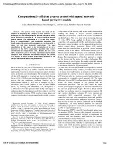
Remark: The achieved bounds on the filtered tracking error can be kept small enough by proper selection of design parameters αq , cij , li , q = 1, ⋯, 4, i = 1, ⋯, p, j = 1, ⋯, ρi − 1, and hidden layer neuron numbers. Increasing the design parameters α2,4 may lead to a more stable control scheme; however it may worsen the tracking performance. Furthermore, increasing cij and α1,3 improve the tracking performance; however it yields more oscillations in transition period. In addition, increasing the NN node numbers cause higher accuracy; however too much increment of node numbers increases the computational burden and it may also cause over fitting. To sum up, one solution for achieving good tracking performance is selecting large values for α1,3 and cij , small values for α2,4 , and using trial and error method for choosing the neuron numbers. IV. E XPERIMENTAL R ESULTS In order to evaluate effectiveness of the proposed control methodology, a WAM robot in real time robotic laboratory of Amirkabir university is considered as a case study Fig. 1. WAMs are good examples of multivariable nonlinear systems with completely coupled dynamics, parameter variations, and high degrees of nonlinearity. The considered WAM is a 6 DoF robot with two arms. Each arm is equipped with three MAXON EC motors. The first two joints motors are placed on the main body of the robot. The third joints motors are also placed on the first links and their signals are transmitted to the joints via crank mechanism.
1.5
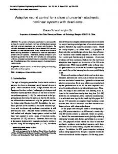
q1 and q1d
1
q13 q13d
q11
0.5
q11d
0 −0.5 −1 0
Fig. 1: Real time laboratory of Amirkabir university of technology’s whole arm manipulator.
q12d q12
10
20 T ime[sec]
30
40
Fig. 2: Tracking performance of the first arm joint positions; dashed lines joint positions q1j , solid lines desired joint positions q1jd .
Dynamics of each arm can be expressed as, 1.5
q¨i = −Mi−1 (qi )Ci (qi , q˙i )q˙i − Mi−1 (qi )gi (qi ) + Mi−1 (qi )τi ,
if t ≤ 30 ∶ ⎡ q ⎢ i1d ⎢ qid = ⎢ qi2d ⎢ ⎢ qi3d ⎣
⎤ ⎡ −0.4 sin(0.5t) ⎥ ⎢ ⎥ ⎢ −0.63 ⎥=⎢ ⎥ ⎢ ⎥ ⎢ 0.174 + 0.002326t2 − 0.000051703t3 ⎦ ⎣
⎤ ⎥ ⎥ ⎥, ⎥ ⎥ ⎦
if t > 30 ∶ ⎡ q ⎤ ⎡ ⎤ ⎢ i1d ⎥ ⎢ −0.4 sin(0.5t) ⎥ ⎢ ⎥ ⎢ ⎥ −0.63 ⎥, qid = ⎢ qi2d ⎥ = ⎢ ⎢ ⎥ ⎢ ⎥ ⎢ qi3d ⎥ ⎢ ⎥ 0.872 ⎣ ⎦ ⎣ ⎦ where qijd , i = 1, 2, j = 1, 2, 3, denote the desired trajectory of the jth joint position of the ith arm. Initial conditions of the arms are selected arbitrarily. The employed NN is assumed to have 15 neurons in the hidden layer and weights of the NN are initialized by random numbers. Other design parameters of the designed controller are selected as α1,3 = 65, α2,4 = 0.1, c11 = 110, c21 = 70, c31 = 110, c41 = 110, , c51 = 70, , c61 = 110, li = 5, i = 1, ⋯, 6. The designed controller is implemented and experimental results are depicted in Figs. 2-5. From Fig. 2, it can be
1 q2 and q2d
where i = 1, 2; Mi (qi ) ∈ Rni ×ni denotes the inertia matrix of ith robot; Ci (qi , q˙i ) ∈ Rni ×ni represents the Coriolis and centrifugal forces matrix; gi ∈ Rni and τi ∈ Rni are the gravitational forces vector and the control generalized, respectively. Note that since the suggested controller does not rely on analytical model of the robot, there is no need for deriving its model. It is also woth pointing out that since the robot inertia matrix is positive definite, its inverse is also positive definite. As a result, Assumption 2 is satisfied and the proposed control scheme is applicable. The desired trajectories of the arms joints are selected identical, which are given by:
q23 q23d
q21
0.5
q21d
0 −0.5 −1 0
q22d q22
10
20 Time [sec]
30
40
Fig. 3: Tracking performance of the second arm joint positions; dashed lines joint positions q2j , solid lines desired joint positions q2jd .
seen that the positions of the first, second, and third joints of the first arm track the desired trajectory vector accurately. Tracking performance of the second arm is also illustrated in Fig. 3. Figs. 2-3 indicate that the tracking errors converge to small neighborhood of the origin, while the robot dynamics are assumed to be unknown. Furthermore, the implemented torques of the motors of the first and second arms are shown in Fig. 4 and Fig. 5, respectively. For uncertain nonlinear systems some valuable schemes have been developed. However, a fundamental assumption underlying most of these schemes is that the system states and inputs are not completely coupled or the system nonlinearities are known a priori [2], [6]-[8]. On the other hand, the proposed control methodologies in the field of robotic systems are also designed based on some nice properties of robotic systems; therefore they are just applicable to special robotic systems [16]. Moreover, experimental results demonstrate superiority of the suggested approach in both theoretical and practical aspects and its easy implementation
10
u21
u11
10 0 −10 0
10
20 Time [sec]
30
0 −10 0
40
10
(a) u12
u22 10
20 Time [sec]
30
30
40
30
40
0 −10 0
40
10
(b)
20 Time [sec]
(b)
10
10
u23
u13
40
10
0
0 −10 0
30
(a)
10
−10 0
20
Time [sec]
10
20 Time [sec]
30
40
(c)
0 −10 0
10
20
Time [sec]
(c)
Fig. 4: Torque inputs of the first arm; (a) first joint, (b) second joint, (c) third joint.
Fig. 5: Torque inputs of the second arm; (a) first joint, (b) second joint, (c) third joint.
and reliability.
[7] T. Li, R. Li, and D. Wang, ”Adaptive neural control of nonlinear MIMO systems with unknown time delays,” Neurocomputing, vol. 78, no. 1, pp. 83-88, Feb. 2012. [8] B. Karimi and M. B. Menhaj, ”Non-affine nonlinear adaptive control of decentralized large-scale systems using neural networks,” Info. Sci., vol. 180, no. 17, pp. 3335-3347, Sep. 2010. [9] V. Panwar, N. Kumar, N. Sukavanam, and J. Borm, ”Adaptive neural controller for cooperative multiple robot manipulator system manipulating a single rigid object,” Applied Soft Comput., vol. 12, no. 1, pp. 216-227, Jan. 2012. [10] L. Yu, S. Fei, L. Sun, and J. Huang, ”An adaptive neural network switching control approach of robotic manipulators for trajectory tracking,” Int. J. Comput. Math., vol. 91, no. 5, 2014. [11] B. Yang and A. J. Calise, ”Adaptive control of a class of nonaffine systems using neural networks,” IEEE Trans. Neural Netw., vol. 18, no. 4, pp. 1149-1159, 2007. [12] S. S. Ge and J. Zhang, ”Neural network control of nonaffine nonlinear systems with zero dynamics by state and output feedback,” IEEE Trans. Neural Netw., vol. 14, no. 4, pp. 900-918, 2003. [13] M. Chen and S. S. Ge, ”Direct adaptive neural control for a class of uncertain nonaffine nonlinear systems based on disturbance observer,” IEEE Trans. Cybern., vol. 43, no. 4, pp. 1213-1225, Aug. 2013. [14] K. Esfandiari, F. Abdollahi, and H. A. Talebi, ”Adaptive control of uncertain nonaffine nonlinear systems with input saturation using neural networks,” IEEE Trans. Neural Netw. Learn. Syst., vol. 26, no. 10, pp. 2311-2322, Oct. 2015. [15] K. Esfandiari F. Abdollahi, and H. A. Talebi, ”Stable adaptive output feedback controller for a class of uncertain non-linear systems,” IET Control Theory Appl., vol. 9, no. 9, pp. 1329 1337, Jun. 2015. [16] H. A. Talebi, R. V. Patel, and H. Asmer, ”Neural network based dynamic modeling of flexible-link manipulators with application to the ssrms,” J. Robotic Syst., vol. 17, no. 7, pp. 385-401, Jul. 2000. [17] J. Mahdavi, M. R. Nasiri, A. Agah, and A. Emadi, ”Application of neural networks and state-space average to dc/dc pwmconverters in sliding-mode operation,” IEEE/ASME Trans. Mechatron., vol. 10, no. 1, pp. 60-67, Feb. 2005. [18] H. Khalil, Nonlinear Systems, 3rd ed. Englewood Cliffs, NJ: PrenticeHall, 2001.
V. C ONCLUSIONS In this research, an adaptive neural controller was designed for a class of multivariable nonaffine nonlinear systems. The considered class covered MIMO/SISO nonaffine/affine systems with complete/partial interconnections which exhibits no internal dynamics. In order to use full capabilities of NNs, weights of both layers were assumed to be adjustable. The suggested control scheme ensured that all signals of the closed-loop system were ultimately bounded, and the tracking error converged to an adjustable neighborhood of the origin. Finally, the suggested methodology was implemented on a completely coupled MIMO robotic system, and the experimental results verified the effectiveness of the presented theoretical discussions. R EFERENCES [1] M. Krstic, I. Kanellakopoulos, and P. V. Kokotovic, Nonlinear and Adaptive Control Design. New York: Wiley, 1995. [2] W. Gao and R. Selmic, ”Neural network control of a class of nonlinear systems with actuator saturation,” IEEE Trans. Neural Netw., vol. 17, no. 1, pp. 147-156, Jan. 2006. [3] C. Hua, C. Yu, and X. Guan, ”Neural network observer-based networked control for a class of nonlinear systems,” Neurocomputing, vol. 133, pp. 103-110, Jun. 2014. [4] K. Esfandiari, F. Abdollahi, and H. A. Talebi, ”A stable nonlinear in parameter neural network controller for a class of saturated nonlinear systems,” in Proc. 19th IFAC World Congress, pp. 2533-2538, Aug. 2014. [5] Y. Wen and X. Ren, ”Neural networks-based adaptive control for nonlinear time-varying delays systems with unknown control direction,” IEEE Trans. Neural Netw. , vol. 22, no. 10, pp. 1599-1612, Oct. 2011. [6] S. Tong, S. Sui, and Y. Li, ”Fuzzy adaptive output feedback control of mimo nonlinear systems with partial tracking errors constrained,” IEEE Trans. Fuzzy Syst., vol. 23, no. 4, pp. 729-742, Aug. 2015.