Neural Network-Based Control Strategies Applied to a Fed-Batch ...

INTERNATIONAL JOURNAL OF COMPUTATIONAL INTELLIGENCE VOLUME 3 NUMBER 3 2006 ISSN 1304-2386

Neural Network-Based Control Strategies Applied to a Fed-Batch Crystallization Process P. Georgieva and S. Feyo de Azevedo1 crystallization industry, modern model-based control strategies attract more industrial attention as being potentially capable of overcoming the problem of repeatability and driving the process to its optimal state [1], [2]. However, the crystallisation occurs through the complex mechanisms of particle nucleation, subsequent particle growth and agglomeration or aggregation, phenomena that are physically not well understood therefore their reliable modelling is still a challenging task [3]. For example many of the reported crystallizer models neglect the agglomeration effect but it leads in general to biased estimation of CV and MA [4]. Development of a reliable model facilitates effectively all subsequent steps in process optimization, control and operation monitoring. There are two main modelling paradigms - analytical (based on the first principles rules) which has been the traditional way of process modelling since many years and data-driven (based on the process data) which became nowadays practically meaningful due to the rapid growth of computational resources. One of the most successful data-driven modelling techniques are the artificial neural networks (ANNs). Their ability to approximate complex non-linear relationships without prior knowledge of the model structure makes them a very attractive alternative to the classical modelling techniques [5]- [7]. The purpose of this paper is twofold. On one hand we discuss the benefits of applying hybrid strategy for dynamic modelling of an industrial fed-batch evaporative sugar crystallization process combining analytical and ANN approaches. This mixed strategy is termed as Knowledge Based Hybrid Modelling (KBHM). On the other hand, we introduce two control alternatives based on an ANN nonlinear model to regulate the process such that the supersaturation tracks a desired, process-dependent reference signal. Model Predictive Control (MPC) and Feedback Linearizing Control (FLC) are comparatively considered and evaluated with respect to closed loop performance, constrains feasibility and computational efforts.

Abstract—This paper is focused on issues of process modeling and two model based control strategies of a fed-batch sugar crystallization process applying the concept of artificial neural networks (ANNs). The control objective is to force the operation into following optimal supersaturation trajectory. It is achieved by manipulating the feed flow rate of sugar liquor/syrup, considered as the control input. The control task is rather challenging due to the strong nonlinearity of the process dynamics and variations in the crystallization kinetics. Two control alternatives are considered – model predictive control (MPC) and feedback linearizing control (FLC). Adequate ANN process models are first built as part of the controller structures. MPC algorithm outperforms the FLC approach with respect to satisfactory reference tracking and smooth control action. However, the MPC is computationally much more involved since it requires an online numerical optimization, while for the FLC an analytical control solution was determined.

Keywords— artificial neural networks, nonlinear model control, process identification, crystallization process I. INTRODUCTION

T

HE phenomenon of crystallisation occurs in a large group of pharmaceutical, biotechnological, food and chemical processes. These kind of industrial productions are usually performed in a batch or fed-batch mode which is related with the formulation of a control problem in terms of economic or performance objective at the end of the process. The crystallisation quality is evaluated by the particle size distribution (PSD) at the end of the process which is quantified by two parameters - the average (in mass) particle size (MA) and the coefficient of particle variation (CV). The main challenge of the batch production is the large batch to batch variation of the final PSD. This lack of process repeatability is caused mainly by improper control policy and results in final product recycling and loss increase. Due to the highly competitive nature of the today’s P. Georgieva is with the Department of Electronics and Telecommunications/IEETA, University of Aveiro, 3810-193 Aveiro, Portugal (corresponding author, phone: +351-234-370531; fax: +351-234370-545; e-mail: [email protected]). S. Feyo de Azevedo is with the Department of Chemical Engineering, Faculty of Engineering, University Porto, Rua Dr. Roberto Frias s/n, 4200-465 Porto, Portugal (e-mail: [email protected]).

IJCI VOLUME 3 NUMBER 3 2006 ISSN 1304-2386

II. PROCESS OPERATION Crystallisation occurs through the mechanisms of nucleation, growth and agglomeration. The process is characterised by strongly non-linear and non-stationary dynamics and can be divided into several sequential phases. Charging. During the first phase the pan is partially filled

224

© 2006 WORLD ENFORMATIKA SOCIETY

INTERNATIONAL JOURNAL OF COMPUTATIONAL INTELLIGENCE VOLUME 3 NUMBER 3 2006 ISSN 1304-2386

with a juice containing dissolved sucrose (termed liquor). Concentration. The next phase is the concentration. The liquor is concentrated by evaporation, under vacuum, until the supersaturation reaches a predefined value. At this stage seed crystals are introduced into the pan to induce the production of crystals. This is the beginning of the third (crystallisation) phase. Crystallisation (main phase). In this phase as evaporation takes place further liquor or water is added to the pan in order to guarantee crystal growth at a controlled supersaturation level and to increase total contents of sugar in the pan. In most cases, due to economical reasons, the liquor is replaced by other juice of lower purity (termed syrup). Tightening. The fourth phase consists of tightening which is principally controlled by the evaporation capacity. The pan is filled with a suspension of sugar crystals in heavy syrup, which is dropped into a storage mixer. At the end of the batch, the final massecuite undergoes centrifugation, where final refined sugar is separated from the (mother) liquor. The unit contains 15 sensors for the following properties and operating variables: i) inside the pan - massecuite temperatures at three locations; brix of solution; level; massecuite consistency; stirrer current; vacuum pressure and temperature. ii) feed conditions - temperature, brix and flow rate of feed liquor and feed syrup. iii) steam conditions temperature, pressure and flow rate of steam. Brix is the concentration of total dissolved solids (sucrose plus impurities) in the solution. Supersaturation is not a measured variable but can be determined from the available measurements. More details about the process can be found elsewhere [8], [9], [10].

dM c = J cris dt

where Pur f and ρ f

process input. Energy balance The general energy balance model is

dTm = aJ cris + bF f + cJ vap + d dt

parameters incorporating the enthalpy terms and specific heat capacities derived as functions of physical and thermodynamic properties [8].

Population balance Mathematical representation of the crystallization rate can be achieved through basic mass transfer considerations [11] or by writing a population balance represented by its moment equations [12]. Employing a population balance is generally preferred since it allows to take into account initial experimental distributions and, most significantly, to consider complex mechanisms such as those of size dispersion and/or particle agglomeration/aggregation. Hence, the population balance is expressed by the leading moments of PSD in ~ ) since agglomeration must obey mass volume coordinates ( µ i conservation low,

(2)

dM s = Ff ρ f B f Purf − J cris dt

(3)

IJCI VOLUME 3 NUMBER 3 2006 ISSN 1304-2386

d µ% 0 % 1 = B0 − β ′µ% 02 dt 2

(6)

d µ%1 = Gν µ% 0 dt

(7)

d µ% 2 = 2Gν + β ′µ%12 dt

(8)

and the crystallisation rate is determined as

Mass balance The mass of water ), impurities ( M i ), dissolved sucrose ( M s ) and crystals ( M c ) are included in the following set of conservation mass balance equations

dM i = F f ρ f B f (1 − Purf ) dt

(5)

where J vap is the evaporation rate and a, b, c, d are

A. Analytical prior knowledge approach (white box model) The traditional way of process modelling for many years has been by mathematical equations. Since the analytical models capture physical behaviour they have the potential to extrapolate beyond the regions for which the model was constructed. The general first principles model describing a batch crystallisation process consists of three parts [8].

(1)

are the purity (mass fraction of

sucrose in the dissolved solids) and the density of the incoming feed. F f is the feed flowrate considered as the

III. CRYSTALIZATION PROCESS MODELLING

dM w = F f ρ f (1 − B f ) + Fw ρ w − J vap dt

(4)

J cris = ρ c

~ dµ 1 . dt

(9)

~ B0 , Gv and β’ are the kinetic variables nucleation rate,

volume growth rate and the agglomeration kernel, respectively. It is difficult to formulate physically based analytical models for the kinetic variables (Fig. 1). Here, the empirical correlations have a long tradition and there exist in the literature a large number of empirical equations for them [4], [8], [13]. The decision which of them provides the best approximation of the crystallisation process in hand is very difficult.

225

© 2006 WORLD ENFORMATIKA SOCIETY

INTERNATIONAL JOURNAL OF COMPUTATIONAL INTELLIGENCE VOLUME 3 NUMBER 3 2006 ISSN 1304-2386

energy and population balances (1-9) with a feed-forward ANN for modelling the nucleation rate ( B NN ), the growth rate (G NN) and the agglomeration kernel (βNN) (see Fig. 3). The ANN has 4 inputs, 3 outputs and one hidden layer with 9 sigmoid activation functions. The temperature of masecute ( Tm ), the supersaturation (S), the purity of the solution ( Pursol ) and the volume fraction of crystals ( υ c ) are considered as the networks inputs because they all affect directly the kinetic parameters.

G,B, β

Process inputs

Empirical Kinetic model

Population balance (CSD moments)

Mass &energy process outputs balance analytical models

Fig. 1 Analytical model

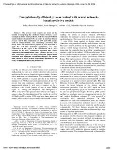
B. ANN (black box model) An obvious advantage of the ANN modelling is its universal character in approximating different physical phenomena with similar computational structure. It saves time and efforts for identifying parameters, in contrast to the case when an analytical model is designed. Therefore ANNs are nowadays known as powerful computing structures for data processing and information storage. However, they have some remarkable disadvantages. The ANN approach suffers of the lack of transparent structure and physical understanding of the network parameters. The resulting black-box (input-output) model in general does not provide the transparency desired to enhance the process understanding. It relies only on the recorded data and does not exploit any other source of knowledge available for the process in hand. A complete FFNN model of the sugar crystallisation was also developed. It has single input single output structure and one hidden layer with 7 sigmoid activation functions (Fig. 2). The input is related to on-line collected physical measurements of the feed flow rate. The network output is the supersaturation for which historical data are also available. The FFNN parameters were tuned applying the LevenbergMarquart optimisation procedure [14].

Process inputs

GNN, BNN, βNN

Hybrid ANN training – sensitivity approach The training of an ANN requires that the network weights are determined in such a way that the error between the network output and the corresponding target output becomes minimal. In the hybrid system, however, the target outputs are not available since the kinetic parameters are not measured. Therefore, an alternative training procedure was required. Our solution was to build a hybrid ANN training structure where the network outputs go through some fixed (known) part of the analytical model and to compare this hybrid model output with the available data (Fig. 4).

Pursol ANN process model

Tm Supersaturation

GNN ~ hyb µ 0

BNN

ANN

βNN

υc

Fig. 2 FFNN model

(

dMc hyb ~ hyb = f 2 GNN ,µ 0 dt

Mchyb

Sensitivity equations

~ hyb, GNN, BNN,βNN µ 0

eobs =Mc −Mc obs

)

dµ~0 hyb = f1 (B NN , β NN ) dt

⎡∂Mchyb / ∂G⎤ ⎢ ⎥ etr = eobs ⎢∂Mchyb / ∂B⎥ ⎢ ∂Mchyb / ∂β ⎥ ⎣ ⎦

C. Knowledge-based hybrid modeling (grey box model) Knowledge-based hybrid modelling (KBHM) is a quite efficient alternative of the two modelling techniques discussed above [15]. The idea of KBHM is to complement the analytical model with the data-driven approach. In the design of such models it is possible to combine theoretical and experimental knowledge as well as process information from different sources: theoretical knowledge from physical and mass conservation laws; experimental data from laboratory plant experiments; experimental data from real plant experiments; data from regular process operation; knowledge and experience from qualified process operators. The clear advantages of KBHM compared with the data-based modelling are first with respect to more physical transparency of the model parameters and secondly less training data is required [16]. Our solution for a KBHM of the crystallization process combines a partial analytical model reflecting the mass,

IJCI VOLUME 3 NUMBER 3 2006 ISSN 1304-2386

Mass &energy process outputs balance analytical models

Fig. 3 KBHM

S

Feed flowrate

Population balance (CSD moments )

ANN

hyb

Mcobs

Fig. 4 Hybrid ANN training procedure

The error for updating the network weights is a function of the observed error and the gradient of the hybrid model output with respect to the ANN output. The mass of crystals is considered as most appropriate to serve as a target output in the hybrid ANN training. According to equations (4), (6) and (9), the mass balance of crystals can be rewritten as

dM c hyb ~ hyb )1 / 3 ( M hyb ) 2 / 3 G NN = 3(k v ρ c )1 / 3 (µ 0 c dt

(10)

(10) is incorporated in the hybrid training structure but in

226

© 2006 WORLD ENFORMATIKA SOCIETY

INTERNATIONAL JOURNAL OF COMPUTATIONAL INTELLIGENCE VOLUME 3 NUMBER 3 2006 ISSN 1304-2386

order to integrate it the zero moment ( µ~0 ) is required. Therefore its balance equation is also involved in the network training stage ( see also (6) ) , 2 hyb dµ~0 hyb 1 = B NN − β NN ⎛⎜ µ~0 ⎞⎟ . dt 2 ⎝ ⎠

dχ B ∂f ∂f = ~1 χ B + 1 , dt ∂B ∂µ 0 dχ β

(11)

dt

Superscripts hyb and NN are used to point out variables obtained during the hybrid network training. The network outputs give estimates of the growth rate, nucleation and agglomeration kinetic parameters. These estimates are propagated through (10-11). The error signal for updating the network parameters is

[

etr = eobs λ G

λB

λβ

]

T

∂f ∂f = ~1 χ β + 1 , ∂µ0 ∂β f 1 = B NN −

where

χβ =

∂µ~0 . ∂β

(12)

λG =

∂M chyb ∂G

(14)

λB =

∂M chyb ∂B

(15)

λβ =

∂M chyb . ∂β

(16)

min

The gradients (14-16) can be computed through integration of the sensitivity equations

dλG ∂f 2 ∂f = λ + 2 , λ G (0) = 0 hyb B dt ∂G ∂M c

dt

=

∂M c hyb

u min ≤u (t ) ≤u max

(17)

~ hyb ∂µ ( 0 ) , λ B (0) = 0 ∂B

(18)

~ hyb ∂f 2 ∂µ 0 , λ β (0) = 0 , λβ + ~ hyb ∂β ∂µ 0

0

χB =

∂µ~0 , ∂B

and

J = ϕ ( x(t ), u (t ), P),

(22)

x& = f ( x(t ), u (t ), P ), 0 ≤ t ≤t f , x(0) = x0

(23.1)

y (t ) = h( x(t ), P)

(23.2)

g j ( x) = 0,

j = 1,2,...... p

(24.1)

v j ( x) ≤ 0,

j = 1,2,......l

(24.2)

(19) where (22) is the performance index, (23) is the process model, function f is the state-space description, function h is the relationship between the output and the state, P is the vector of possibly uncertain parameters and t f is the final

0

batch time. x(t ) ∈ R n , u (t ) ∈ R m and y (t ) ∈ R p are the state, the manipulated input and the control output vectors, respectively. The manipulated inputs, the state and the control outputs are subject to the following constraints,

β´, respectively. In order to determine them the same strategy is applied leading to integration of the following sensitivity equations with zero initial conditions

IJCI VOLUME 3 NUMBER 3 2006 ISSN 1304-2386

1 ˆ NN ⎛ ~ hyb ⎞ 2 β ⎜ µ0 ⎟ , 2 ⎝ ⎠

subject to:

Note, that while λ G can be straightforward obtained, λ B ~ and λ depend on the gradients of µ~ with respect to B and β

(21)

A. Problem formulation Nonlinear model predictive control (NMPC) is an optimisation-based multivariable constrained control technique that uses a nonlinear dynamic model for the prediction of the process outputs [17]. At each sampling time the model is updated on the basis of new measurements and state variables estimates. Then the open-loop optimal manipulated variable moves are computed over a finite (predefined) prediction horizon with respect to some performance index, and the manipulated variables for the subsequent prediction horizon are implemented. Then the prediction horizon is shifted or shrunk by usually one sampling time into the future, and the previous steps are repeated. The optimal control problem in the NMPC framework can be mathematically formulated as:

(13)

with the gradient of the hybrid model output with respect to the network outputs

∂f 2

χ β ( 0) = 0 ,

IV. ANN-BASED MODEL PREDICTIVE CONTROL

eobs = M c obs − M c hyb

dλ β

(20)

The network parameters were tuned applying the LevenbergMarquart optimization procedure [12].

It is obtained by multiplying the observed error

dλ B ∂f 2 ∂f 2 = λB + hyb ~ dt ∂M c ∂µ 0 hyb

χ B (0) = 0

227

© 2006 WORLD ENFORMATIKA SOCIETY

INTERNATIONAL JOURNAL OF COMPUTATIONAL INTELLIGENCE VOLUME 3 NUMBER 3 2006 ISSN 1304-2386

x(t ) ∈ Χ, u (t ) ∈ Ζ, y (t ) ∈ Υ in which Χ , Z and Y are convex n

m

descent algorithm is the conjugate gradient algorithm (with many variations) [23] where a search is performed along conjugate directions, which produces generally faster convergence than steepest descent directions

p

and closed subsets of R , R and R . g j and v j are the equality and inequality constrains with p and l dimensions respectively.

wk +1 = wk + α k rk

B. Identification stage – ANN learning algorithms

All of the conjugate gradient algorithms start out by searching in the steepest descent direction (negative of the gradient) on the first iteration

ANNs have been successfully applied in the modelling, estimation, monitoring and control of dynamical systems. Their approximation capabilities make them a promising alternative for modelling nonlinear systems and for implementing general-purpose nonlinear controllers [18], [19],[20]. There are typically two stages involved when using ANN for control: process identification and control design. At the identification stage, an ANN model of the process dynamics is developed. The ANN model uses previous inputs and previous process outputs to predict future values of the process output. The prediction error between the process output and the ANN output is used as an ANN training signal. The network is trained usually offline in batch mode, using data collected from the operation of the plant or generated by a reliable model. At the control design stage, the ANN plant model is used to design the controller. Among various ANN training algorithms the backpropagation (BP) algorithm is the most widely implemented for modeling purposes [21]. In fact, BP is a generalization of least mean square (LMS) algorithm of Widrow and Hoff, [22] for multilayer feedforward ANN. Standard BP is a gradient descent algorithm in which the network weights are moved in the steepest descent direction i.e. along the negative of the gradient of the performance index. This is the direction in which the performance index is decreasing most rapidly. The term backpropagation refers to the manner in which the gradient is computed for nonlinear multilayer networks. Properly trained BP networks tend to give reasonable answers when presented with inputs that they have never seen. This generalization property makes it possible to train a network on a representative set of input/ target pairs and get good results without training the network on all possible input/output pairs. One (k) iteration of the gradient steepest descent algorithm can be written as wk +1 = wk − α k g k , g k =

∂Pk , ∂wk

r01 = − g 0

(27)

A line search is then performed to determine the optimal distance to move along the current search direction. Then the next search direction is determined so that it is conjugate to previous search directions. The general procedure for determining the new search direction is to combine the new steepest descent direction with the previous search direction rk = − g k + β k rk −1 .

(28)

The various versions of conjugate gradient are distinguished by the manner in which the constant β k is computed. For the Fletcher-Reeves update the procedure is

βk =

g kT g k . g kT−1 g k −1

(29)

This is the ratio of the norm squared of the current gradient ( g k ) to the norm squared of the previous gradient ( g k −1 ). For the Polak-Ribiére update, the constant β k is computed by

βk =

∆g kT−1 g k . g kT−1 g k −1

(30)

This is the inner product of the previous change in the gradient ( ∆g kT−1 ) with the current gradient divided by the norm squared of the previous gradient. A third alternative to the steepest descent algorithm for fast optimization is the Newton’s method [14]. The basic step of Newton’s method is

(25)

wk +1 = wk − H k−1 g k , H k =

where wk is a vector of current weights and biases, gk is the current gradient of the performance index Pk and αk is the learning rate. There are two different ways in which this algorithm can be implemented: incremental mode and batch mode. In the incremental mode, the gradient is computed and the weights are updated after each input is applied to the network. In the batch mode all of the inputs are applied to the network before the weights are updated. It turns out that, although the performance function decreases most rapidly along the negative of the gradient, this does not necessarily produce the fastest convergence. An alternative to the steepest

IJCI VOLUME 3 NUMBER 3 2006 ISSN 1304-2386

(26)

∂Pk2 ∂wk ∂wk

(31)

where H k is the Hessian matrix (second derivatives) of the performance index Pk at the current values (k) of the weights and biases. Newton’s method often converges faster than steepest descent and conjugate gradient methods. Unfortunately, it is complex and expensive to compute the Hessian matrix for feedforward ANN. There is a class of algorithms that is based on Newton’s method, but which doesn’t require calculation of second derivatives. These are

228

© 2006 WORLD ENFORMATIKA SOCIETY

INTERNATIONAL JOURNAL OF COMPUTATIONAL INTELLIGENCE VOLUME 3 NUMBER 3 2006 ISSN 1304-2386

action over a specified (control) horizon that minimize the following performance index

called quasi-Newton methods. They update an approximate Hessian matrix at each iteration of the algorithm. The update is computed as a function of the gradient. LevenbergMarquardt algorithm, implemented in our application, is one of the celebrating quasi-Newton methods. It is designed to approach second-order training speed without having to compute the Hessian matrix. When the performance function has the form of a sum of squares of the errors (as it is typical in training a feedforward NN), then the Hessian matrix can be approximated as

H k = J kT J k

NN MPC

Optimization procedure

ANN process model

(32) Process (KBHM)

where J k is the Jacobian matrix that contains first derivatives of the network errors ( ek ) with respect to the weights and biases ∂e J k = k ; ek = y m − t . ∂wk

Fig. 5 ANN-based model predictive control (ANN-MPC)

min

u min ≤ [u (t + k ), u (t + k +1,.....u (t + c )) ]≤ u max

(33)

p

k =1

]

−1

J Tk ek

future control signal, which are limited by u min and u max and

(35)

parameterized as peace wise constant. λ1 and λ2 determine the contribution of the sum of the squares of the output error and the control increments over the performance index. The length of the prediction horizon is crucial for achieving tracking and stability. For small values of p the tracking deteriorates but for high p values the bang-bang behaviour of the process input might be a real problem. The MPC controller requires a significant amount of on-line computation, since the optimization (36) is performed at each sample time to compute the optimal control input. At each step only the first control action is implemented to the process (in this case to the simulation KBHM).

When the scalar µ is zero, this is just Newton’s method, using the approximate Hessian matrix. When µ is large, this becomes gradient descent with a small step size. Newton’s method is faster and more accurate near an error minimum, so the aim is to shift towards Newton’s method as quickly as possible. Thus, µ is decreased after each successful step (reduction in performance function) and is increased only when a tentative step would increase the performance function. In this way, the performance function will always be reduced at each iteration of the algorithm.

V. NUMERICAL IMPLEMENTATION OF ANN-MPC

C. Closed loop ANN-MPC structure The particular closed loop MPC structure considered in this work is illustrated in Fig. 5. For the simulation purposes the KBHM process model introduced in section III was implemented as the simulation model (see Fig. 3). The controller consists of the feed forward ANN process model discussed also in section III (see Fig. 2) and an optimization block. The ANN model predicts future process responses to potential control signals over the prediction horizon. The predictions are supplied to the optimization block to determine the values of the control

IJCI VOLUME 3 NUMBER 3 2006 ISSN 1304-2386

k =1

The prediction horizon p is the number of time steps over which the prediction errors are minimized and the control horizon c is the number of time steps over which the control increments are minimized, yr is the desired response and ym is the network model response. u (t + k ), u (t + k + 1),.....u (t + c) are tentative values of the

The computation of the Jacobian matrix is less complex than computing the Hessian matrix. The LevenbergMarquardt algorithm updates the weights in the following way

[

2

(36)

(34)

wk +1 = wk − J Tk J k + µI

c

λ1 ∑ ( yr (t + k ) − ym (t + k ) ) − λ2 ∑ (u (t + k − 1) − u (t + k − 2) )

where ym is the network output vector and t is the target vector. Then the gradient can be computed as

g k = J k ek

2

P =

The numerical implementation of ANN-MPC control is schematically presented in Fig. 6. The control problem is simulated in Matlab/Simulink framework as a set of modules. The Matlab NN Toolbox is also required. The controller is designed as an independent block and the process is simulated as a KBHM model. The KBHM model is coded as an Sfunction required by Simulink. First, the ANN process model is identified in a specific Plant Identification window (Fig. 7). In this window are specified the network architecture (number of inputs, outputs, layers, type and number of neurons in a

229

© 2006 WORLD ENFORMATIKA SOCIETY

INTERNATIONAL JOURNAL OF COMPUTATIONAL INTELLIGENCE VOLUME 3 NUMBER 3 2006 ISSN 1304-2386

Simulation results are summarized in Fig. 10 and Fig. 11. The process manipulated input (the feed flow rate) is depicted in subplot (a) and the process controlled output (the supersaturation) is depicted in subplot (b) for control horizon c=4 and prediction horizon p=10 (Fig. 10) and p=4 (Fig. 11). The peace-wise constant output reference was determined based on the optimal profile derived by an off-line dynamic optimization [24]. During the stages of concentration and feeding with liquor, the reference was set at Sref=1.15 and afterwards was reduced to Sref=1.05. A smooth transition between the two levels was determined to overcome possible overreaction of the tracking controller. The graphics show satisfactory reference tracking with an acceptable smooth behaviour of the control input which stays within the technological constrains defined with umax=0.015 [m3/s]. Higher the prediction horizon better is the tracking but to the expense of more vivid manipulated input. For higher values of p (>10), the control action faced saturation problems.

layer), training data limitations and training parameters (number of epochs, training algorithm).

Fig. 6 ANN MPC – simulation scheme

M PC

(a) Training (input-output) data; ANN error and output Fig. 7 Plant Identification block

The ANN is trained in a batch mode by LevenbergMarquardt algorithm (35). An example of data generated by applying a series of random step inputs to the KBHM and recording the model output (the supersaturation) is depicted in Fig. 8. Data is divided into training, validation and simulation portions. Before introducing to the ANN, it is normalized in the range (-1,1) and after processing over the network, the network outputs are denormalized. On the same figure one can observe the ANN response and error to the different data sets. On Fig 9 is summarised the learning process. While the training and the validation errors are significantly different (Fig.9a), the generalization properties of the network are not reliable and the training has to continue. The learning is stopped when the training and the validation errors are sufficiently close (Fig.9b). The identified ANN model (which is part of the final MPC structure) consists of one hidden layer with 7 sigmoid squashing activation functions and one output linear layer.

IJCI VOLUME 3 NUMBER 3 2006 ISSN 1304-2386

(b) Validation (input-output) data; ANN error and output

230

© 2006 WORLD ENFORMATIKA SOCIETY

INTERNATIONAL JOURNAL OF COMPUTATIONAL INTELLIGENCE VOLUME 3 NUMBER 3 2006 ISSN 1304-2386

b) Supersaturation profile and its ref. trajectory Fig. 10 ANN-MPC simulations p=10, c=4

(c) Simulation (input-output) data; ANN error and output Fig. 8 Data generation and ANN processing

a) a) Feed rate profile and its max allowed value

b)

Fig. 9 Testing and validation error

b) Supersaturation profile and its ref. trajectory Fig. 11 ANN-MPC simulations p=4, c=4

VI. ANN FEEDBACK LINEARISING CONTROL In this section we report the numerical realization of the second control structure, an ANN-based feedback linearising control (FLC). The central idea is to design a controller that can transform nonlinear system dynamics into linear dynamics by canceling the nonlinearities. It is assumed that the process

a) Feed rate profile and its max allowed value

IJCI VOLUME 3 NUMBER 3 2006 ISSN 1304-2386

231

© 2006 WORLD ENFORMATIKA SOCIETY

INTERNATIONAL JOURNAL OF COMPUTATIONAL INTELLIGENCE VOLUME 3 NUMBER 3 2006 ISSN 1304-2386

u ( k + 1) =

can be reliably represented by the general Nonlinear Autoregressive-Moving Average (NARMA) model:

ref (k + d ) − f [ y (k ),..... y (k − n + 1), u (k ),...u (k − m + 1)] g [ y (k ),..... y (k − n + 1), u ( k ), u ( k − 1)...u (k − m + 1)]

y (k + d ) = N [ y ( k ), y (k − 1),..... y ( k − n + 1), u ( k ), u ( k − 1),...u (k − m + 1)] (37)

(42) The numerical implementation of ANN-FLC is schematically presented in Fig. 13. Similar to the ANN-MPC it is simulated in Matlab/Simulink. The “best” results obtained are depicted in Fig. 14. Attempts to improve the tracking lead to bang-bang control input behaviour.

where u (k ) is the system input, y (k ) is the system output and N(.) is a nonlinear functional relationship. The first step in the procedure is to find an ANN that approximates N(.). The next step is to develop a nonlinear controller u (k ) = G[ y (k ),..... y ( k − n + 1), ref ( k + d ), u (k − 1),...u (k − m + 1)] (38) such that the system output follows some reference trajectory

y (k + d ) = ref (k + d )

(39)

However, the training of an ANN to approximate the function N(.) requires the use of dynamic backpropagation. It appeared to be a quite slow procedure that provoked computational and convergence problems. Therefore to reduce the computational burden we had to apply a different scenario. The solution, proposed by Narendra [20], is to assume an approximate NARMA model of the system in a companion form

Fig. 12 ANN approximation of f(.) and g(.)

ANN FeedbackLinearizing Control

~ y (k + d ) = f [ y (k ), y (k − 1),..... y (k − n + 1), u (k ), u (k − 1),...u (k − m + 1)] + g [ y (k ), y (k − 1),..... y (k − n + 1), u (k − 1),...u (k − m + 1)]u (k ) (40) and train two ANNs to approximate the two nonlinear functions f(.) and g(.), as it is shown in Fig. 12. The main advantage of (40) is that analytical solution exists for the control input that causes the system output to follow the reference signal. The resulting controller has the following form

S_REF.mat

Clock1 0.015

Reference

Ff Clock

Const1

From File1 f Plant Output

g

Control Signal Feed Flow

Ff

S

Supersaturation

crystal_smodel

Fig. 13 ANN feedback linearizing control – simulation scheme

u (k ) =

ref (k + d ) − f [ y (k ),..... y (k − n + 1), u (k − 1),...u (k − m + 1)] g [ y (k ),..... y (k − n + 1), u (k − 1),...u ( k − m + 1)] (41)

Using directly (41) can cause realization problems, because one must determine the control input u (k ) based on the output at the same time y (k ) . To avoid this implementation obstacle d must be equal or higher than 2 and the control action in this case is a) Feed rate profile and its max allowed value

IJCI VOLUME 3 NUMBER 3 2006 ISSN 1304-2386

232

X(2Y) Graph

© 2006 WORLD ENFORMATIKA SOCIETY

INTERNATIONAL JOURNAL OF COMPUTATIONAL INTELLIGENCE VOLUME 3 NUMBER 3 2006 ISSN 1304-2386

REFERENCES [1] [2] [3] [4] [5] [6] [7]

b) Supersaturation profile and its ref. trajectory

[8]

Fig. 14 ANN feedback liberalizing control simulations [9]

VII. CONCLUSIONS

[10]

The application of ANNs at two stages of sugar crystallization process automation, namely modelling and control, is presented in this paper. At the modelling stage, a knowledge based hybrid model (KBHM) of the process was designed that possesses the advantages of both analytical and pure data based process models. The KBHM offers a reasonable compromise between the extensive efforts to get a fully parameterised structure, as are the analytical models and the poor generalisation of the complete data-based modelling approaches. At the control stage, two ANN-based control algorithms were studied - model predictive control (MPC) and feedback linearizing control (FLC). MPC algorithm outperforms the FLC approach with respect to satisfactory reference tracking and smooth control action. However, the MPC is computationally much more involved since it requires an online numerical optimization, while for the FLC, an analytical control solution was determined. Since the ANN models capture the nonlinear process nature, both methods have the potential advantage over the control methods based on linear models. It should, however, be pointed out that variations of initial conditions and disturbances during the batch are not treated in this paper but they are most probably to appear in the reality. Work on it is now in progress.

[11] [12] [13] [14] [15] [16] [17] [18]

[19] [20] [21] [22]

ACKNOWLEDGMENT This work was pursued in the framework Project BatchPro HPRN-CT-2000-0039. It financed by the Portuguese Foundation for Technology within the activity of the Research Aveiro, which is gratefully acknowledged.

[23]

of EC RTN was further Science and Unit IEETA-

IJCI VOLUME 3 NUMBER 3 2006 ISSN 1304-2386

[24]

233

J. B. Rawlings, S. M. Miller, and W. R. Witkowski., “Model identification and control of solution crystallization processes: a review”, Ind. Eng. Chem. Res., 32(7):1275-1296, July 1993. Nagy Z. K. and R. D. Braatz,. Robust nonlinear model predictive control of batch processes. AIChE J., 49:1776-1786, 2003. Fujiwara, M. Z. K. Nagy, J. W. Chew, and R. D. Braatz First-principles and direct design approaches for the control of pharmaceutical crystallization. J. of Process Control, 15:493-504, 2005 (invited). Feyo de Azevedo, S., Chorão, J., Gonçalves, M.J. and Bento, L., 1994, On-line Monitoring of White Sugar Crystallization through Software Sensors. Int. Sugar JNL., 96:18-26. S. Haykin S. (1994), Neural Networks: A comprehensive foundation, Prentice Hall, UK. Russell N.T. and H.H.C. Bakker (1997), Modural modelling of an evaporator for long-range prediction, Artificial Intelligence in Engineering, 11, 347-355. Zorzetto L.F.M., R. Maciel Filho and M.R. Wolf-Maciel (2000), Process modelling development through artificial neural networks and hybrid models, Computers and Chemical Engineering, 24, 1355-1360. Georgieva P., Meireles, M. J. and Feyo de Azevedo, S., 2003, KBHM of fed-batch sugar crystallization when accounting for nucleation, growth and agglomeration phenomena. Chem Eng Sci, 58:3699-3711. Georgieva P., Feyo de Azevedo, M. J. Goncalves, P. Ho (2003a). Modelling of sugar crystallization through knowledge integration. Eng. Life Sci., WILEY-VCH 3 (3) 146-153. Georgieva P., J. Peres, R. Oliveira, S. Feyo de Azevedo (2003c): Process Modelling Through Knowledge Integration Competitive and Complementary Modular Principles. Workshop on Modeling and Simulation in Chemical Engineering, 30 June-4 July, Coimbra, Portugal, Proc. CIM 22, 1-8. Ditl, P., Beranek L., & Rieger, Z. (1990). Simulation of a stirred sugar boiling pan. Zuckerind., 115, 667-676. A.D. Randolph, M.A. Larson, Theory of Particulate Processes – Analyses and Techniques of Continuous Crystallization, Academic Pres, 1988. P. Lauret, H. Boyer, J.C. Gatina, Hybrid modelling of a sugar boiling process, Control Engineering Practice, 8, 2000, 299-310. Hagan M. T., M. Menhaj (1994), “Training feedforward networks with the Marquardt algorithm,” IEEE Transactions on Neural Networks, vol. 5, no.6, pp. 989–993. D.C. Psichogios, L. H. Ungar, A hybrid neural network - first principles approach to process modelling, AIChE J., 38(10), 1992, 1499-1511. Graefe, J., Bogaerts, P., Castillo, J., Cherlet, M., Werenne, J., Marenbach, P., & Hanus, R. (1999). A new training method for hybrid models of bioprocesses. Bioprocess Engineering, 21, 423-429. Mayne D.Q., J.B. Rawlings, C.V. Rao, P.O.M. Scokaert (2000), Constrained model predictive control: stability and optimality, Automatica, 36 789-814. Cabrera J.B.D., K.S. Narendra (1999), Issues in the Application of Neural Networks for Tracking Based on Inverse Control, IEEE Transactions on Automatic Control Special Issue on Neural Networks for Control, Identification, and Decision Making, 44(11), 2007-2027. Haykin S. (1994), Neural Networks: A comprehensive foundation, Prentice Hall, UK. Lingji Ch., K.S. Narendra (2001), Nonlinear Adaptive Control Using Neural Networks and Multiple Models, Automatica, Special Issue on Neural Network Feedback Control, 37(8), 1245-1255. Rumelhart, D.E., & McClelland, J. L., (1986). Parallel Distributed Processing, Cambridge, MA: MIT Press. Widrow B., & M.E. Hoff, Adaptive switching circuits, IRE WESCON (New York. Convention Record.), 96--104, 1966. Hagan M. T., H. B. Demuth, M. H. Beale (1996), Neural NetworkDesign, Boston, MA: PWS Publishing. V. Galvanauskas, P. Geogieva, S. Feyo de Azevedo, Dynamic optimization of industrial sugar crystallization process based on a hybrid (mechanistic +ANN) model, accepted for publication to IJCNN, Vancouver, Canada, June 2006.

© 2006 WORLD ENFORMATIKA SOCIETY