Nat. Hazards Earth Syst. Sci., 11, 2341–2353, 2011 www.nat-hazards-earth-syst-sci.net/11/2341/2011/ doi:10.5194/nhess-11-2341-2011 © Author(s) 2011. CC Attribution 3.0 License.
Natural Hazards and Earth System Sciences
Neural network based tomographic approach to detect earthquake-related ionospheric anomalies S. Hirooka1 , K. Hattori1 , M. Nishihashi2 , and T. Takeda3 1 Graduate
School of Science, Chiba University, Chiba, Japan Research Institute, Tsukuba, Japan 3 Department of Computer Science, The University of Electro-Communications, Tokyo, Japan 2 Meteorological
Received: 27 November 2010 – Revised: 23 February 2011 – Accepted: 4 July 2011 – Published: 26 August 2011
Abstract. A tomographic approach is used to investigate the fine structure of electron density in the ionosphere. In the present paper, the Residual Minimization Training Neural Network (RMTNN) method is selected as the ionospheric tomography with which to investigate the detailed structure that may be associated with earthquakes. The 2007 Southern Sumatra earthquake (M = 8.5) was selected because significant decreases in the Total Electron Content (TEC) have been confirmed by GPS and global ionosphere map (GIM) analyses. The results of the RMTNN approach are consistent with those of TEC approaches. With respect to the analyzed earthquake, we observed significant decreases at heights of 250–400 km, especially at 330 km. However, the height that yields the maximum electron density does not change. In the obtained structures, the regions of decrease are located on the southwest and southeast sides of the Integrated Electron Content (IEC) (altitudes in the range of 400–550 km) and on the southern side of the IEC (altitudes in the range of 250– 400 km). The global tendency is that the decreased region expands to the east with increasing altitude and concentrates in the Southern hemisphere over the epicenter. These results indicate that the RMTNN method is applicable to the estimation of ionospheric electron density.
1
Introduction
Liu et al. (2006a) statistically examined the relationship between foF2 by ionosonde in Taiwan and 184 M ≥ 5.0 earthquakes in Taiwan that occurred during the period from 1994 to 1999. They found a significant decrease in foF2 in the Correspondence to: S. Hirooka (
[email protected])
afternoon one to five days before the investigated earthquakes. They also reported that significant decreases in Total Electron Content derived by GPS (GPS-TEC) appeared one to five days prior to M ≥ 6.0 earthquakes in Taiwan (Liu et al., 2004). The GPS-TEC results can also provide a spatial distribution of anomalous regions that may be associated with earthquakes. However, it is difficult to obtain information on vertical distributions of electron density. In order to clarify the physical mechanism of earthquakerelated ionospheric anomalies, the investigation of threedimensional electron density distributions is very important. This requires a tomographic approach (Garcia-Fernandez et al., 2003; Saito et al., 2007). These methods require an ionospheric model and/or a large amount of data for computation, although model-free reconstruction is essential in the case of disturbed ionospheric problems. In this sense, the Residual Minimization Training Neural Network (RMTNN) tomography proposed by Ma et al. (2005a, b) and Takeda et al. (2007) is a good algorithm because it does not require a model for an initial value and requires only a small number of data. Therefore, the RMTNN algorithm is used in the present paper. Sumatra island is one of the most seismically active regions in the world. Numerous large earthquakes occur along the Sumatra trench every year. A total of 70 M > 6.0 earthquakes have occurred along the Sumatra trench after the 2004 Sumatra-Andaman Earthquake (Mw = 9.2). A number of researchers have reported various anomalous electromagnetic phenomena that may be associated with large earthquakes in the Indonesia region. These anomalous changes are classified into two types: co-/post-seismic phenomena and pre-seismic phenomena (Hattori, 2009). Here, we introduce a number of aspects related to the large earthquakes around the Sumatra island. First, co-/post-seismic phenomena have been reported. Iyemori et al. (2005) reported geomagnetic pulsations that may have been caused by the 2004
Published by Copernicus Publications on behalf of the European Geosciences Union.
2342 Sumatra-Andaman earthquake. The observed geomagnetic pulsations suggest the existence of a large current in space caused by acoustic waves based on surface displacements. Otsuka et al. (2006) reported the enhancement of GPS-TEC on the north side of the epicenter 14 to 40 min after the 2004 Sumatra-Andaman earthquake. They concluded that the enhancement is caused by acoustic waves generated by the earthquake. Heki et al. (2006) also suggested that the vertical displacement of the ruptures propagates to the ionosphere by means of an acoustic wave and generates TEC anomalies. Liu et al. (2006b) detected two giant ionospheric disturbances by a digital Doppler sounder network in Taiwan. They reported that the first disturbance was excited primarily by Rayleigh waves and that the second disturbance was attributable to the coupling of the atmospheric gravity waves (AGW) excited by broad crustal uplift together with the subsequent large tsunami waves. Balasis and Mandea (2007) investigated magnetic and electron density data observed by CHAMP for the 2004 and 2005 Sumatra earthquakes. They observed some specific features after two earthquakes having periods of approximately 16 and 30 s. The results favored an external source origin for the 30 s pulsation. Hasbi et al. (2009) observed TEC oscillations with periods of 5 to 10 min approximately 10 to 24 min after the 2005 Sumatra Earthquakes (M = 8.6 and M = 6.7), which had horizontal propagation velocities of 922 to 1259 m s−1 . In addition, magnetic field measurements revealed rapid fluctuations of 4 to 5 s shortly after the earthquake, followed by a Pc5 pulsation of 4.8 min approximately 11 min after the event. A good correlation was found between the filtered TEC and Pc5 pulsation, suggesting that the acoustic pulse generated near the epicenter propagates upward to ionospheric heights and induces disturbances in the ionospheric E and F regions. The pre-seismic phenomena around Sumatra island are described in the following. Anomalous TEC changes possibly preceding large earthquakes around Taiwan have been described above, and similar results have been reported by Hattori et al. (2009), who statistically examined the relationship between TEC by global ionosphere map (GIM) and 184 M ≥ 5.0 earthquakes around Sumatra island that occurred during the period from 1998 to 2008. They found a significant decrease in TEC at 3 to 17 days before the earthquakes of interest. They also reported that significant decreases in TEC appeared five days prior to the 2004 Sumatra-Andaman earthquake. Furthermore, the anomalous propagation of VLF radio waves has been investigated. For example, Horie et al. (2007) investigated data for subionospheric VLF waves from the Australian VLF transmitter NWC (19.8 kHz) at the Japanese receiving stations at Chofu, Chiba, and Kochi. The VLF amplitude data at Japanese stations indicated a reduction in amplitude and an enhancement of the nighttime amplitude fluctuation before the earthquake. Molchanov et al. (2006) investigated the reception on board the DEMETER satellite of the VLF signals transmitted by the NWC. They found a drop in the signals (scattering spot) connected Nat. Hazards Earth Syst. Sci., 11, 2341–2353, 2011
S. Hirooka et al.: Neural network based tomographic approach with the occurrence of the 2004 Sumatra-Andaman Earthquake. The extension of the “scattering spots” zone was significantly large (1000–5000 km). As mentioned above, although the 2004 SumatraAndaman Earthquake is a very interesting target, the number of useful GPS data is insufficient for the present study. Therefore, we consider herein the 2007 Southern Sumatra earthquake (M = 8.5) because of the availability of GPS network data and because significant decreases in GIM-TEC have been detected (Hattori et al., 2009). In the present paper, we demonstrate the performance of the developed RMTNN method and investigate the 3D structure of possible earthquake-related ionospheric anomalies associated with the 2007 Southern Sumatra earthquake (M = 8.5) by GPS-TEC. In order to verify the reliability of results obtained by the developed RMTNN method, we compared estimated electron densities with occultation data observed by FORMOSAT-3/C. 2
Ionospheric tomography using a neural network
The residual minimization training neural network (RMTNN) is a multilayer neural network that is trained by minimizing an object function composed of an appropriately prepared residual of equations (Ma et al., 2000; Liaqat et al., 2003). In this method, we reconstruct three-dimensional ionospheric electron density distributions as a computer tomographic image by using the ability of a multilayer neural network system to approximate an arbitrary function. 2.1
Basic function
A slant TEC (Mannucci et al., 1998) along a ray path between a GPS satellite and a ground receiver is defined as the integrated value of ionospheric and plasmaspheric electron density, including instrumental bias, as follows: Z rj j N (r)ds + Bi + B j Ii = (1) ri
j
where Ii is the slant TEC, N (r) is the electron density, and Bi and B j are the instrumental bias of the i-th ground receiver and the j -th satellite bias, respectively. In order to determine N (r), which represents the electron density at a position r, a neural network is constructed. The input parameter of the proposed neural network is r, and the output is N (r). In order to evaluate the residuals of the integral equation, the equation is discretized as j
Ii ≈
Q X
j
αq N (r) + Bi + B j + Pi
(2)
q=1
where q and α denote a sampling point and the corresponding weight for the numerical integration, respectively, Q is www.nat-hazards-earth-syst-sci.net/11/2341/2011/
S. Hirooka et al.: Neural network based tomographic approach
2343
Fig. 2. Ionospheric electron density distribution at longitude 100◦ E. (a) Original electron density distribution using the NeQuick model. (b) Reconstructed electron density distribution.
hmF2, and Nsion is the observed NmF2 value. Therefore, the overall objective function E is derived as (5)
E = gE1 + E2 Fig. 1. Schematic diagram of the data flow for ionospheric tomography using RMTNN. In the figure, 1w is the update value for the main neural network, and 1Bi and 1B j are the instrumental bias of the ith ground receiver and the j -th satellite bias, respectively.
the total number of sampling points on a ray path, and P is the contribution of the plasmaspheric electron density to the slant TEC I . We herein define altitudes of 100 to 700 km as the ionosphere and altitudes above 700 km as the plasmasphere modeled by the simple diffusive equilibrium model (Angerami and Thomas, 1964). In order to estimate the electron density N (r), we take the squares of the residuals of the above integral equations as the objective function of the neural network. The objective function E1 is given as
E1 =
Q X
j
j
(αq N (r) + Bi + B j + Pi − Ii )2 .
2.3
Procedure
Figure 1 shows a schematic diagram of the data flow for ionospheric tomography by RMTNN. The RMTNN system is composed of the main neural network for reconstruction and additional neural networks consisting of single neurons for instrumental bias (Bi , B j ). The receiver bias Bi and the satellite bias B j are estimated at the time of the reconstruction. The procedure used to obtain the electron density is as follows: 1. Provide initial weights with random values. 2. Provide the input data (coordinates) and the desired output data (observed STEC values) for the neural network.
(3)
q=1
2.2
where g is a balance parameter between the GPS and ionosonde data.
Assimilation of ionosonde data
The disadvantage of ionospheric tomography using the ground GPS receivers is the difficulty in obtaining sufficient vertical resolution due to a lack of paths. In order to solve this problem, we use information on the peak electron density (NmF2) and the corresponding height (hmF2) observed by an ionosonde station for restriction. The neural network was trained using these data through the conventional supervised back propagation algorithm (Rumelhart et al., 1986). The object function E2 for the ionosonde data is given by
3. Compute the output value of the main neural network and evaluate the objective function E1. 4. Update the weight values by the back propagation method (for RMTNN) as follows. For the objective function E1, the weight updating process of the main neural network is derived in clusters for the n-th path as 1w = −η ∂E1 ∂w Q P ∂I N N j ≈ −η (InN N + Bi + B j + Pi − In ) ∂Nn q = −η
q=1 Q P
q=1
E2 =
S X
(Ns (r s ) − Nsion )2
(4)
s=1
where S is the number of ionosondes, Ns is the output of the neural network for the corresponding position that gives www.nat-hazards-earth-syst-sci.net/11/2341/2011/
j (InN N + Bi + B j + Pi
− In )αq
∂N q ∂w
(6)
∂N q ∂w
where n represents the ray path (i, j ), InN N is a line integral along the numerically obtained n-th path using the output data of the neural network, w is the weight of the main neural network, and η is the learning rate. Return to Step 2 until the all ray path is processed. Nat. Hazards Earth Syst. Sci., 11, 2341–2353, 2011
2344
Fig. 3. Differences in the integrated electron content (IEC) between the original and the reconstructed data at 150 km intervals from altitudes of 100 to 700 km. (a) IEC at altitudes of 100 to 250 km, (b) IEC at altitudes of 250 to 400 km, (c) IEC at altitudes of 400 to 550 km altitudes, and (d) IEC at altitudes of 550 to 700 km.
5. Provide the input data (a coordinate of hmF2 above the ionosonde station) and the desired output data (an observed NmF2 value). 6. Compute the output values and evaluate the objective function E2. 7. Update the weight values by the general back propagation method (Rumelhart et al., 1986) for objective function E2. 8. Return to Step 2 until a criterion is satisfied. In the present paper, the number of iterations is fixed as 10 000. Regarding the error E, after 10 000 iterations, E < 10−2 . The criterion of E is empirically determined by numerical simulations. If the iteration process is not convergent, change the initial weight values and retry the iteration process. In the present paper, we used data for a period of 15 min for the reconstruction. Therefore, we assume that the electron density distribution is constant during this period. We also assume that the electron density is constant within an area of 0.5 degrees latitude by 0.5 degrees longitude and 30 km in altitude. 3
Simulation
Ma et al. (2005b) demonstrated the effectiveness of reconstructing the electron density using the RMTNN algorithm Nat. Hazards Earth Syst. Sci., 11, 2341–2353, 2011
S. Hirooka et al.: Neural network based tomographic approach
Fig. 4. Map of the epicenter of the 2007 Southern Sumatra earthquake, GPS ground receivers, and Kototabang ionosonde station.
for the GEONET in Japan for quiet periods. The target of the present study is the Sumatra region, Indonesia, and the reconstruction is difficult because of the small number of GPS receivers. Therefore, we investigated the numerical simulation. For the simulations, the actual positions of the GPS receivers and the ionosonde station around Sumatra and model STEC values are used. The model STEC values are generated by the NeQuick model (Radicella et al., 2001; Nava et al., 2008). NeQuick model is a threedimensional, time-dependent ionospheric electron density model developed by the Aeronomy and Radiopropagation Laboratory of the Abdus Salam International Centre for Theoretical Physics (ICTP) and the Institute for Geophysics and Meteorology of the University of Graz. We compared the reconstructed electron density distribution with that derived from the NeQuick model. In this simulation, the dataset of 18:00–18:15 UT, 9 September 2007 is prepared. For the RMTNN, 22 GPS receivers from SuGAr, two GPS receivers from IGS, and the observation from the ionosonde station located in Kototabang are used. The reconstructed region is 10◦ S–10◦ N and 90◦ E–110◦ E in latitude and longitude and 100 to 700 km in altitude. The model and reconstructed distributions are shown in Fig. 2a and b, respectively. These figures are drawn for a vertical cross section at a fixed longitude of 100◦ E. The reconstruction data agrees well with the model data. Figure 3 shows the integrated electron content (IEC) at altitude intervals of 150 km from 100 to 700 km for a detailed comparison of the model and the reconstruction. The IECs at altitude ranges of 250 to 400 km, 400 to 550 km, and 550 to 700 km exhibit only slight errors, except at the www.nat-hazards-earth-syst-sci.net/11/2341/2011/
S. Hirooka et al.: Neural network based tomographic approach
2345
Fig. 5. Variations of GIM-TEC*, Kp index, and Dst index from 1 September to 13 September 2007 for various longitudes. The solid green line shows the time at which the earthquake occurred. The blue areas indicate periods during which a significant decrease in GIM-TEC* over −2σ occurred at multiple stations. Red frames mark significant decreases in GIM-TEC* around the epicenter.
edge of the reconstruction area. The IEC at altitudes in the range of 100 to 250 km is underestimated compared to other altitudes and appears to be latitude dependent. This seems to be due to a lack of restrictions on electron density at lower altitudes. However, the difference is within ±1 TECU at all IECs. Therefore, it is safe to say that the RMTNN reconstruction is applicable for sparse conditions.
receivers, and the ionosonde is shown in Fig. 4. Before applying the proposed RMTNN method, we confirm the existence of possible TEC anomalies before the earthquake. After reconstruction of the electron density, we compare the results with GPS occultation data obtained by satellite.
4
In order to estimate the TEC anomaly associated with the 2007 Southern Sumatra earthquake, we used TEC data sets from the GIM published by the Center for Orbit Determination in Europe (CODE). We hereinafter refer to GIM-TECas TEC from GIM data and GPS-TEC as TEC from GPS data. The computation of the GIM-TEC is performed as follows. The original spatial resolution of GIM is 2.5◦ in latitude and
Application to the 2007 Southern Sumatra earthquake
The Southern Sumatra earthquake (M = 8.5 and depth 34 km) occurred on 12 September 2007. The epicenter was located at 4.520◦ S, 101.374◦ E, off the south coast of Sumatra, Indonesia. A map of the epicenter, the selected GPS www.nat-hazards-earth-syst-sci.net/11/2341/2011/
4.1
TEC anomalies before the 2007 Southern Sumatra earthquake
Nat. Hazards Earth Syst. Sci., 11, 2341–2353, 2011
2346
S. Hirooka et al.: Neural network based tomographic approach
Fig. 6. Variations of GIM-TEC*, Kp index, and Dst index from 1 September to 13 September 2007 for various latitudes. The solid green line shows the time at which the earthquake occurred. The blue areas indicate periods during which a significant decrease in GIM-TEC* over −2σ occurred at multiple stations. Red frames mark significant decreases in GIM-TEC* around the epicenter.
5.0◦ in longitude, and the temporal resolution is 2 h. We performed linear interpolation to obtain a resolution of 1 hour at a certain resolution. We computed the mean GIM-TEC values for the previous 15 days and the associated standard deviation as a reference at specific times. Then, the normalized GIM-TEC (GIM-TEC*) was defined as follows: GIM TEC(t) − GIM TECmean (t) GIM TEC ∗ (t) = σ (t)
4.2 (7)
where GIM TEC(t) is the extracted GIM data at time t, GIM TECmean (t) is the mean value for the previous 15 days, and σ (t) is the associated standard deviation. Figures 5 and 6 show the variations in GIM TEC* in terms of the longitude and latitude, respectively. The corresponding variations in the Kp and Dst indices are also shown in both figures. Geomagnetic conditions were found to be relatively quiet during the analyzed period. The GIM TEC* around the epicenter exceeded the lower threshold of −2σ on 4 and 9 September, which was eight and three days before the earthquake. In particular, the decrease at 07:00–08:00 UT (14:00–15:00 LT) on 9 September was significant. Figure 7 indicates the disturbed area derived from GIM-TEC and GPS-TEC investigations, and the disturbed area is found to extend 10 degrees Nat. Hazards Earth Syst. Sci., 11, 2341–2353, 2011
in latitude and 40 degrees in longitude. Based on the above results, there was a possible TEC anomaly before the earthquake. Therefore, the proposed RMTNN method was applied to the earthquake in order to investigate the structure of pre-seismic ionospheric anomaly. Results of RMTNN tomography
The 24 selected GPS receivers, including 22 stations from SuGAr and two stations from IGS, and the ionosonde station (Kototabang) for the restriction, are shown in Fig. 4. In the present paper, we focus on the period of 07:30–07:45 UT (14:30–14:45 LT) on 9 September 2007, during which an abnormal TEC decrease was detected by GIM-TEC*. In order to clarify the anomalous changes in three-dimensional electron density distributions, we computed the difference between the reconstructed data on 9 September and the model data that is constructed by the median value through 15-day backward computations. The reconstructed region is 10◦ S– 10◦ N in latitude and 90◦ E–110◦ E in longitude and 100 to 700 km in altitude, which is the same area used in the simulation.
www.nat-hazards-earth-syst-sci.net/11/2341/2011/
S. Hirooka et al.: Neural network based tomographic approach
Fig. 7. Spatial distribution of anomalous GIM-TEC* and GPSTEC* on 9 September 2007. The red star and the solid red line indicate the epicenter and magnetic equator, respectively. Pink circles and orange triangles indicate points/stations at which GIM-TEC* and GPS-TEC* values, respectively, produced anomalies. Purple circles and blue triangles indicate positions at which GIM-TEC* and GPS-TEC* values, respectively, did not produce anomalies. Note that GPS-TEC* was calculated directly by data observed from the GPS receiver as well as GIM-TEC*.
Figure 8 shows the difference in the IEC at altitudes of 100 to 700 km between the observed data and the model data. The IEC (100–700 km) is found to decrease significantly in the Southern Hemisphere, including over the epicenter. This region corresponds to the regions of Figs. 5 through 7 derived by GIM-TEC*. Furthermore, a region in which the IEC increased exists in the northwest region. Figure 9 shows the IEC at altitude intervals of 150 km from 100 to 700 km. The IEC over altitudes of 100 to 250 km indicates that the density decreases in the southwest region, including the epicenter. On the other hand, an increase occurs over the Sumatra-Java islands. The IECs at altitudes of 250 to 400 km and 400 to 550 km decrease significantly around the epicenter. The IEC at altitudes of 550 to 700 km decreases slightly, except in the southwest and in regions east of the epicenter. The ionospheric electron density profile above the epicenter obtained from the tomographic data is shown in Fig. 10. The solid line indicates the profile on 9 September, and the dashed line represents the median profile computed from the reconstructed data during 25 August and 8 September. The observed electron density on September 9 is 40 % of the median value at the peak electron density. And, hmF2 is similar in both cases at an altitude of 330 km. Moreover, the electron density profile observed on 9 September is lower than first quartile value except below 230 km altitude. Figure 11 shows the longitude-altitude and latitude-altitude cross sections, www.nat-hazards-earth-syst-sci.net/11/2341/2011/
2347
Fig. 8. Difference in the integrated electron content (altitudes of 100 to 700 km) between the observed data and the reference data with the 15-day backward median.
which include the epicenter. In addition, Fig. 12 shows only the region in which the difference exceeded the Inter Quartile Range (IQR) in Fig. 11. The results also show a significant decrease in the electron density at approximately 330 km. The area of this decrease expands eastward with altitude and is concentrated in the Southern Hemisphere over the epicenter. Moreover, in order to determine whether the outliers arise from incidental errors, we performed tomography around the period of 07:30–07:45 UT. Figures 13 (1) and 13 (2) show the anomalous features (i.q. Fig. 11) for the periods of 07:15–07:30 UT and 07:45–08:00 UT, respectively. These distributions of anomalies are similar to those shown in Fig. 11, which suggests that the obtained results (Figs. 9 through 12) are reasonable. 4.3
Evaluation of the electron density estimated by FORMOSAT-3 data
In order to validate the electron density distribution obtained by the RMTNN algorithm, we compare the vertical electron density profiles derived by tomography with FORMOSAT-3/C radio occultation measurements (Lei et al., 2007). FORMOSAT-3/C is composed of six microsatellites, each of which houses a GPS occultation experiment. The accuracy of the ionospheric electron density profile observed by FORMOSAT-3/C is extremely high (Lei et al., 2007). However, the observable time and space depends on the positional relationship of the satellites. In the present study, we analyze the occultation data for the afternoon period of 06:00–09:00 UT (13:00–16:00 LT) during 25 August and 9 September. These data provide the electron density profile for the 9 September and the 15-day backward median Nat. Hazards Earth Syst. Sci., 11, 2341–2353, 2011
2348
S. Hirooka et al.: Neural network based tomographic approach
Fig. 9. Differences in the integrated electron content (IEC) between the observed and the reference data at 150 km intervals from altitudes of 100 to 700 km. (a) IEC at altitudes of 100 to 250 km, (b) IEC at altitudes of 250 to 400 km, (c) IEC at altitudes of 400 to 550 km altitudes, and (d) IEC at altitudes of 550 to 700 km.
for the day. The investigated orbits of the satellite are in the region of 5◦ S–15◦ N and 80◦ E–120◦ E, as shown in Fig. 14. In this region, a significant decrease in GIM-TEC* was detected, as shown in Fig. 15, which shows the electron density profiles obtained by FORMOSAT-3/C. The F2 peak density on 9 September was found to be decreased significantly (by approximately 25 %) compared to the median density. The hmf2 is approximately the same in both cases and at 340 km. The tendency of this profile is consistent with that derived using the RMTNN method (Fig. 10). However, the estimations by the RMTNN tomography and by FORMOSAT-3/C below 200 km are different, and the RMTNN estimation provides lower values. This tendency is also in agreement with the results of previous studies (Hsiao et al., 2009, 2010). Fig. 10. Ionospheric electron density profile obtained using the RMTNN method. The solid line indicates the profile from the reconstructed data at 07:30–07:45 UT on 9 September 2007. The dashed and dotted lines indicate the median and the first and third quartile values, respectively, of the reconstructed data at 07:30– 07:45 UT from 25 August to 8 September 2007.
Nat. Hazards Earth Syst. Sci., 11, 2341–2353, 2011
5
Conclusion and discussion
In the present paper, we applied the RMTNN method to estimate the electron density distribution of the ionosphere using STEC and ionosonde data. The analyzed day is three days before the 2007 Southern Sumatra earthquake. Regions of significantly reduced 15-day backward median values of electron density at the same local time are recognized in the www.nat-hazards-earth-syst-sci.net/11/2341/2011/
S. Hirooka et al.: Neural network based tomographic approach
2349
Fig. 11. Example of electron density distributions (07:30–07:45 UT). The red dots indicate the projection of the epicenter. Left panel indicates the IECs. (a) Longitudinal difference in electron density between the observed data and the reference data at the same latitude of epicenter (4.520◦ S). (b) Latitudinal difference in electron density between the observed data and the reference data at the same longitude of the epicenter (101.374◦ E).
Fig. 12. Example of electron density distribution in which the electron density exceeds the IQR (07:30–07:45 UT). Black areas indicate region in which the electron density is smaller than the IQR. Left panel indicates the IECs. (a) Longitudinal difference in electron density between the observed data and the reference data at the same latitude of epicenter (4.520◦ S). (b) Latitudinal difference in electron density between the observed data and the reference data at the same longitude of the epicenter (101.374◦ E).
TEC, IEC, and profile analyses using reconstructed tomographic data. The characteristic of the reduction for the TEC analysis is consistent with the characteristics of the GIMTEC and GPS-TEC. The results for the IEC indicate that significant decreases occur at altitudes of 250 to 400 km, especially at 330 km. However, the height that yields the maximum electron density remains the same. The obtained structure is such that a region of significantly reduced 15day backward median values of electron density exists in the southwest and southeast side of the IEC (altitude: 400 to 550 km) and in the southern side of the IEC (altitude: 250 to 400 km). The global tendency is that this region expands to the east with increasing altitude and is concentrated in the Southern Hemisphere over the epicenter.
www.nat-hazards-earth-syst-sci.net/11/2341/2011/
Anomalous pre-seismic features obtained by GIM/GPSTEC and tomographic TEC/ IEC exhibited good agreement with the results of previous studies. Hattori et al. (2009) reported GPS/GIM-TEC anomalies during the 2004 SumatraAndaman Earthquake. They found an anomalous reduction in GPS/GIM-TEC during the afternoon five days before the earthquake, and reported that the region of decreased electron density expanded 30 degrees in latitude and 40 degrees in longitude from the epicenter. Meanwhile, Liu et al. (2009) reported a reduction in GIM-TEC during the afternoon of 6–4 and three days before the 2008 Wenchuan earthquake (Mw = 7.9) and that the region spread 10–15 degrees in latitude and 15–30 degrees in longitude. Similarly, we observed anomalous decreases in GIM/GPS-TEC around the epicenter during the afternoon 3 days before the earthquake and
Nat. Hazards Earth Syst. Sci., 11, 2341–2353, 2011
2350
S. Hirooka et al.: Neural network based tomographic approach
Fig. 13. Example of electron density distributions (1) 07:15–07:30 UT, (2) 07:45–08:00 UT. The red dots indicate the projection of the epicenter. Left panel indicates the IECs. (a) Longitudinal difference in electron density between the observed data and the reference data at the same latitude of epicenter (4.520◦ S). (b) Latitudinal difference in electron density between the observed data and the reference data at the same longitude of the epicenter (101.374◦ E).
that the anomalous area spread 10 degrees in latitude and 40 degrees in longitude. The tendency for disturbed areas in time and space is found to be common. Although the reconstruction area obtained by tomography is not sufficient for the estimation of the spatial extent of the anomalous area, the obtained results are consistent with the result of GPS/GIMTEC. In addition, the electron density at hmF2 exhibits a significant decrease, which agrees with previous results obtained by ionosonde (Liu et al., 2006a). The profile obtained from the tomographic reconstruction is compared with that obtained from FORMOSAT-3/C in order to evaluate the performance of the proposed RMTNN method. The results indicate good agreement, with the exception of altitudes in the range of 100 to 200 km. The tendency of the decrease in electron density at approximately 300 km before the occurrence of large earthquakes has been reported (Hsiao et al., 2009, 2010), which suggests the high applicability of the RMTNN method to the estimation of ionospheric electron density.
Nat. Hazards Earth Syst. Sci., 11, 2341–2353, 2011
Differences between the results of the present study and the results of previous studies were also found. Hsiao et al. (2009) reported the three-dimensional ionospheric structures obtained prior to the 2006 Pingtung earthquake using FORMOSAT-3/C. They found decreases in the F2 peak height, significant decreases in the electron density at altitudes of from 300 to 350 km, and increases in the lower altitudes within five days prior to the earthquakes. Similar results have been reported for the 2008 Wenchuan earthquake (Liu et al., 2009; Hsiao et al., 2010). On the other hand, the RMTNN results of the present study indicate no enhancement at lower altitudes. The simulation results also revealed that the IEC at altitudes of 100 to 250 km are slightly underestimated compared to the model. With respect to the peak height, no obvious reduction was found from the profiles derived from the RMTNN and FORMOSAT-3/C data. This indicates that no remarkable reduction in hmF2 occurred for the 2007 Southern Sumatra earthquake. One problem associated with the proposed method is the underestimation of the electron density at lower altitudes. www.nat-hazards-earth-syst-sci.net/11/2341/2011/
S. Hirooka et al.: Neural network based tomographic approach
Fig. 14. Locations of points at which profiles were computed from FORMOSAT-3/C occultation data during 06:00–09:00 on 25 August 2007 and 9 September 2007. The red star indicates the epicenter. The blue line and the black lines represent the trajectories on 9 September 2007 and for the reference data (15-day backward median).
This might arise from the lack of information on the lower ionosphere. Additional information on the bottom sounding and/or lower height data using satellite occultation may be required. These problems must be solved in order to improve the RMTNN method. If these problems are solved, we will be able to estimate the electron distribution at the lower ionosphere and discover the sources of nighttime fluctuations and termination time shifts in subionospheric VLF waves (Horie at al., 2007). Even though these results are preliminary, the RMTNN method reveals an interesting three-dimensional structure that may be associated with the 2007 Southern Sumatra earthquake. Such a structure might provide a key to a possible solution to pre-seismic ionospheric anomalies. Recently, several mechanisms for lithosphere-atmosphere-ionosphere coupling, such as the atmospheric electric field, the atmospheric gravity wave (AGW), and gas emanation, have been proposed (Pulinets and Boyarchuk, 2004; Freund, 2000; Molchanov et al., 2006). If positive holes excited around the epicenter diffuse and outflow from the epicenter, an upward electric field is generated on the surface of the earth (Freund, 2000). The upward electric field and the magnetic field of the earth generate a westward E × B drift of plasma (Kelley, 1989). Then, the reduction of ionospheric electron density occurs east of the epicenter. We observed a significant decrease in electron density east of the epicenter (include over the epicenter) at IEC (250 to 400 km) obtained by tomography. However, the obtained region of decreased electron density did not extend northward from the epicenter and was concentrated at 300 km. These results are inconsistent with www.nat-hazards-earth-syst-sci.net/11/2341/2011/
2351
Fig. 15. Ionospheric electron density profiles obtained from FORMOSAT-3/C. The solid line indicates the profile observed on 9 September. The dashed and dotted lines indicate the median and first and third quartile values calculated during the period from 25 August to 8 September, respectively.
the theory proposed by Pulinets and Legan’ka (2003). They reported that the electric field is transferred into the ionosphere along the magnetic field lines, so that, in most cases, the disturbed region is shifted to the north from the epicenter projection in the southern hemisphere. Therefore, in this case, other factors might need to be considered regarding the relationship between the electric field and ionospheric disturbances. Further investigations of the eastward expansion of regions of anomalous decreases with increasing altitude will be required. Continuous tomographic images can provide dynamic variations of the electron density, which reveal the transport of energy from the lithosphere. In other words, the tomographic approach has the advantage of providing a fine spatial distribution and is important for clarifying the coupling mechanism between earthquake preparation processes and ionospheric anomalies. In the present paper, we considered only three periods (07:15–07:30 UT, 07:30–07:45 UT, and 07:45–08:00 UT) of tomographic results. In order to discuss the development of pre-ionospheric anomalies, longerterm continuous analysis is required. Moreover, in order to enhance the reliability of anomalous structures obtained by tomography, some stochastic test (Huang, 2006) and/or continuous analysis are important. Therefore, improvement of processing efficiency will be required. The proposed RMTNN tomography is useful for the study of not only pre-seismic ionospheric disturbances but also co/post-seismic disturbances and general upper atmospheric phenomena. If RMTNN tomography is used to examine co/post-seismic ionospheric disturbances, clarification of the propagation process of the AGW generated by earthquakes Nat. Hazards Earth Syst. Sci., 11, 2341–2353, 2011
2352 and/or tsunamis in the ionosphere may become possible. The results of the present study indicate the applicability of the RMTNN method to the investigation of ionospheric electron density. Acknowledgements. The authors would like to thank the Scripps Orbit and Permanent Array Center (SOPAC) for GPS data of the International GNSS Service (IGS) and Sumatran GPS Array (SuGAr) stations, the National Institute of Information and Communications Technology, Japan for the ionosonde data at Kototabang, the Center for Orbit Determination in Europe (CODE) for the GIM data, and the World Data Center (WDC) for Geomagnetism, Kyoto University for the Dst and Kp index. We would also like to thank X. F. Ma for his helpful suggestion concerning software development. The present research is supported in part by a Grant-in-Aid for Scientific Research from the Japan Society for Promotion of Science (No. 19403002) and National Institute of Information and Communication Technology (R & D promotion funding international joint research). Edited by: K. Eftaxias Reviewed by: two anonymous referees
References Angerami, J. J. and Thomas, J. O.: Studies of planetary atmospheres, The distribution of electrons and ions in the Earth’s exosphere, J. Geophys. Res., 69, 4537–4560, 1964. Balasis, G. and Mandea, M.: Can electromagnetic disturbances related to the recent great earthquakes be detected by satellite magnetometers?, special issue “Mechanical and Electromagnetic Phenomena Accompanying Preseismic Deformation from Laboratory to Geophysical Scale”, Tectonophysics, 431, 173–195, doi:10.1016/j.tecto.2006.05.038, 2007. Freund, F.: Time-resolved study of charge generation and propagation in igneous rocks, J. Geophys. Res., 105, 11001–11019, 2000. Garcia-Fernandez, M., Hernandez-Pajares, M., Juan, M., Sanz, J., Orus, R., Coisson, P., Nava, B., and Radicella, M.: Combining ionosonde with ground GPS data for electron density estimation, J. Atmos. Sol. Terr. Phys., 65, 683–691, 2003. Hasbi, A. M., Momoni, M. A., Ali, M. A. M., Misran, N., Shiokawa, K., Otsuka, Y., and Yumoto, K.: Ionospheric and geomagnetic disturbances during the 2005 Sumatra earthquakes, J. Atmos. Sol. Terr. Phys., 71, 1992–2005, 2009. Hattori, K.: Electromagnetic Phenomena Possibly Associated with the 2004 Sumatra-Andaman Earthquake, The Institute of Electrical Engineers of Japan, Trans. Fundament Materials, 129A, 345–351, 2009 (in Japanese). Hattori, K., Nishihashi, M., and Liu, J. Y.: Statistical and case studies of ionospheric TEC anomalies related to large earthquakes in Indonesia, Geophys. Res. Abstr., Vol. 11, EGU2009–8376, 2009. Heki, K., Otsuka, Y., Choosakul, N., Hemmakorn, N., Komolmis, T., and Maruyama, T.: Detecttion of ruptures of Andaman fault segment in the 2004 great Sumatra earthquake with coseismic ionospheric disturbances, J. Geophys., Res., 111, B09313, doi:10.1029/2005JB004202, 2006. Horie, T., Yamauchi, T., Yoshida, M., and Hayakawa, M.: The wave-like structures of ionospheric perturbation associated with
Nat. Hazards Earth Syst. Sci., 11, 2341–2353, 2011
S. Hirooka et al.: Neural network based tomographic approach Sumatra earthquake of 26 December 2004, as revealed from VLF observation in Japan of NWC signals, J. Atmos. Sol. Terr. Phys., 69, 1021–1028, 2007. Hsiao, C. C., Liu, J. Y., Oyama, K. I., Yen, N. L., Wang, Y. H., and Miau, J. J.: Ionospheric electron density anomaly prior to the Decenber 26, 2006 M7.0 Pingtung earthquake doublet observed by FORMOSAT-3/COSMIC, Phys. Chem. Earth, Parts A/B/C, 34, 474–478, 2009. Hsiao, C. C., Liu, J. Y., Oyama, K. I., Yen, N. L., Liou, Y. A., Chen, S. S., and Miau, J. J.: Seismo-ionospheric precursor of the 2008 Mw7.9 Wenchuan earthquake observed by FORMOSAT3/COSMIC, GPS Solut., 14(1), 83–89, doi:10.1007/s10291-0090129-0, 2010. Huang, Q.: Search for reliable precursors: A case study of the seismic quiescence of the 2000 western Tottori prefecture earthquake, J. Geophys. Res., 111, B04301, doi:10.1029/2005JB003982, 2006. Iyemori, T., Nose, M., Han, D., Gao, Y., Hashizume, M., Choosakul, N., Shinagawa, H., Tanaka, Y., Utsugi, M., Saito, A., McCreadie, H., Odagi, Y., and Yang, F.: Geomagnetic pulsations caused by the Sumatra earthquake on December 26, 2004, Geophys. Res. Lett., 32, L20807, doi:10.1029/2005GL024083, 2005. Kelley, M. C.: The Earth’s Ionosphere, Elsevier, New York, p. 487, 1989. Lei, J., Syndergaard, S., Burns, A. G., Solomon, S. C., Wang, W., Zeng, Z., Roble, R. G., Wu, Q., Kuo, Y-H, Holt, J. M., Zhang, S-R., Hysell, D. L., Rodrigues, F. S., and Lin, C. H.: Comparison of COSMIC ionospheric measurements with ground-based observations and model predictions: Preliminary results, J. Geophys. Res., 112, A07308, doi:10.1029/2006JA012240, 2007. Liaqat, A., Fukuhara, M., and Takeda, T.: Optimal estimation of parameter of dynamical system by neural network collocation method, Comput. Phys. Commun., 150, 215–234, 2003. Liu, J. Y., Chuo, Y. J., Shan, S. J., Tsai, Y. B., Chen, Y. I., Pulinets, S. A., and Yu, S. B.: Pre-earthquake ionospheric anomalies registered by continuous GPS TEC measurements, Ann. Geophys., 22, 1585–1593, doi:10.5194/angeo-22-1585-2004, 2004. Liu, J. Y., Chen, Y. I., Chuo, Y. J., and Chen, C. S.: A statistical investigation of pre-earthquake ionospheric anomaly, J. Geophys. Res., 111, A05304, doi:10.1029/2005JA011333, 2006a. Liu, J. Y., Tsai, Y. B., Chen, S. W., Lee, C. P., Chen, Y. C., Yen, H. Y., Chang, W. Y., and Liu, C.: Giant ionospheric disturbances excited by the M9.3 Sumatra earthquake of 26 December 2004, Geophys. Res. Lett., 33, L0213, doi:10.1029/2005GL023963, 2006b. Liu, J. Y., Chen, Y. I., Chen, C. H., Liu, C. Y., Chen, C. Y., Nishihashi, M., Li, J. Z., Xia, Y. Q., Oyama, K. I., Hattori, K., and Lin, C. H.: Seismo-ionospheric GPS TEC Anomalies Observed before the 12 May 2008 Mw7.9 Wenchuan Earthquake, J. Geophys. Res., 114, A04320, doi:10.1029/2008JA013698, 2009. Ma, X. F., Fukuhara, M., and Takeda, T.: Neural network CT image reconstruction method for small amount of projection data, Nucl. Instrum. Method Phys. Res., A, 449, 366–377, 2000. Ma, X. F., Maruyama, T., Ma, G., and Takeda, T.: Determination of GPS receiver differential biases by neural network parameter estimation method, Radio Sci., 40, RS1002, doi:10.1029/2004RS003072, 2005a. Ma, X. F., Maruyama, T., Ma, G., and Takeda, T.: Three-
www.nat-hazards-earth-syst-sci.net/11/2341/2011/
S. Hirooka et al.: Neural network based tomographic approach dimensional ionospheric tomography using observation data of GPS ground receivers and ionosonde by neural network, J. Geophys. Res., 110, A05308, doi:10.1029/2004JA010797, 2005b. Mannucci, A. J., Wilson, B. D., Yuan, D. N., Ho, C. H., Lindqwister, U. J., and Runge, T. F.: A global mapping technique for GPS derived ionospheric electron content measurements, Radio Sci., 33, 562–582, 1998. Molchanov, O., Rozhnoi, A., Solovieva, M., Akentieva, O., Berthelier, J. J., Parrot, M., Lefeuvre, F., Biagi, P. F., Castellana, L., and Hayakawa, M.: Global diagnostics of the ionospheric perturbations related to the seismic activity using the VLF radio signals collected on the DEMETER satellite, Nat. Hazards Earth Syst. Sci., 6, 745–753, doi:10.5194/nhess-6-745-2006, 2006. Nava, B., Coisson, P., and Radicella, S. M.: A new version of the NeQuick ionosphere electron density model, J. Atmos. Sol. Terr. Phys., 70, p. 15, doi:10.1016/j.jastp.2008.01.015, 2008. Otsuka, Y., Kotake, N., Tsugawa, T., Shiokawa, K., Ogawa, T., Effendy, Saito, S., Kawamura, M., Maruyama, T., Hemmakorn, N., and Komolmis, T.: GPS detection of total electron content variations over Indonesia and Thailand following the 26 December 2004 earthquake, Earth Planet. Space, 58, 159–165, 2006.
www.nat-hazards-earth-syst-sci.net/11/2341/2011/
2353 Pulinets, S. A. and Boyarchuk, K. A.: Precursors of Earthquakes, Springer, Berlin, Germany, 2004. Pulinets, S. A. and Legan’ka, A. D.: Spatial-Temporal Characteristics of Large Scale Disturbances of Electron Density Observed in the Ionospheric F-Region before Strong Earthquakes, Cosmic Res., 41, 221–229, 2003. Radicella, S. M., and Leitinger, R.: The evolution of the DGR approach to model electron density profiles, Adv. Space Res., 27, 35–40, 2001. Rumelhart, D. E., Hinton, G. E., and Williams, R. J.: Learning internal representations by error propagation, in: Parallel Distributed Processing, MIT Press, 1, 318–362, 1986. Saito, A., Teraishi, S., Ueno, G., Fujita, N., and Tsugawa, T.: GPS Ionospheric Tomography over Japan with Constrained Leastsquares Method, American Geophysical Union, Fall Meeting, abstract #SA13A-1061, 2007. Takeda, T. and Ma, X. F.: Ionospheric Tomography by Neural Network Collocation Method, Plasma Fusion Res., 2, S1015, doi:10.1585/pfr.2.S1015, 2007.
Nat. Hazards Earth Syst. Sci., 11, 2341–2353, 2011