Neural Network Model Reference Adaptive Control of a Surface Vessel Alexander Leonessa and Tannen S. VanZwieten Abstract— A neural network model reference adaptive controller for trajectory tracking of nonlinear systems is developed. The proposed control algorithm uses a single layer neural network that bypasses the need for information about the system’s dynamic structure and provides portability. Numerical simulations are performed using a three degree of freedom nonlinear dynamic model of a surface vessel. The results demonstrate the controller performance in terms of tuning, robustness and tracking.
the tracking error is ultimately bounded when subject to some generalized constraints. The addition of a single layer neural network bypasses the need for information about the system’s dynamic structure and characteristics. The presented control algorithm is tested and tuned using the surface vessel’s nonlinear model presented in [1].
I. INTRODUCTION
In this section we establish definitions, notation, and a key result used later in the paper. Let R denote the set of real numbers, let Rn denote the set of n × 1 real column vectors, let Rn×m denote the set of real n × m matrices, and let (·)T denote transpose. Furthermore, we write ||·|| for the Euclidean vector norm and A ≥ 0 (resp., A > 0) to denote the fact that the Hermitian matrix A is nonnegative (resp., positive) definite. In this paper we consider nonlinear controlled dynamical systems of the form
Research and development on Autonomous Surface Vehicles (ASVs) is motivated by the navigation and communication challenges involved with the use of Autonomous Underwater Vehicles (AUVs). The ASV development objective is to provide real time positioning of and communication with AUVs through the air-sea interface. Guidance and control play an integral part in the ASV’s success, which is a motivating factor for this research. The overall dynamics for a three degree of freedom ASV are modeled and numerically simulated in [1]. Since the modeling trends and dynamical behavior are similar for different surface vessels, using the model developed in [1] will help to quantify the dynamics and performance capabilities of surface vessels in general and facilitate the testing and tuning of the controllers. Furthermore, the model in [1] allows to study the effect of the model nonlinearities on the controller’s performance. The dynamical behaviors of a surface vessel can only be partially depicted using current modeling techniques. These dynamics are especially complicated when the vehicle’s motion is in transient, as when considering a tracking problem where the vessel may be required to follow search patterns or its desired path is constantly being modified. Additionally, the ocean environment is characterized by large, unknown perturbations. These features make it desirable to have a control system that is capable of self-tuning. This paper introduces a neural network model reference adaptive controller which has valuable self-tuning capabilities that allow it to “adapt” to the operating conditions in order to optimize the tracking performance of the closedloop system. The parameter update mechanism is derived using ultimate boundedness theory, which guarantees that Alexander Leonessa is with the Faculty of Mechanical, Materials, and Aerospace Engineering, University of Central Florida, P.O. Box 162450, Orlando, FL 32816 − 2450
[email protected] Tannen S. VanZwieten is a Ph.D. Student in the Department of Mechanical, Materials, and Aerospace Engineering, University of Central Florida, P.O. Box 162450, Orlando, FL 32816 − 2450
[email protected]
II. MATHEMATICAL PRELIMINARIES
x(t) ˙ = F (x(t), u(t)),
x(0) = x0 ,
t ∈ I x0 ,
(1)
where x(t) ∈ D ⊆ Rn , t ≥ 0, is the system state vector, Ix0 ⊆ R is the maximal interval of existence of a solution x(·) of (1), D is an open set, 0 ∈ D, u(t) ∈ U ⊆ Rm , t ≥ 0, is the control input, U is the set of all admissible controls such that u(·) is a measurable function with 0 ∈ U, and F : D × U → Rn is continuous on D × U. Following the notation introduced in [2], consider the following nonlinear autonomous dynamical system x(t) ˙ = f (t, x(t)),
x(0) = x0
t ∈ I x0
(2)
where f : Ix0 × D → Rn is piecewise continuous in t and locally Lipschitz in x. Definition 2.1: [2] The solutions of (2) are uniformly ultimately bounded with ultimate bound ε > 0 if there exists γ > 0 such that, for every δ ∈ (0, γ), there exists T = T (δ, ε) > 0 such that ||x0 || < δ implies ||x(t)|| < ε, t ≥ T. In the case of autonomous systems, we may drop the word “uniformly”. To see how Lyapunov analysis can be used to study ultimate boundedness, we introduce the following theorem. Theorem 2.1: [2] Assume that there exists a continuously differentiable function V : Ix0 × D → R such that α(||x||) ≤ V (t, x) ≤ β(||x||), (t, x) ∈ Ix0 × D, ∂V ∂V + f (t, x) ≤ −W (x), ||x|| ≥ µ > 0, ∂t ∂x
(3) (4)
where α(·) and β(·) are class K functions, W : D → R is a continuous positive definite function, and µ > 0 is such that Bα−1 (β(µ)) (0) ⊂ D. Then the solutions of (2) are ultimately bounded with ultimate bound ε , α−1 (β(µ)).
EFF
xe
y CG
ye x
yb
III. MODELING
ψ
In this section we present a mathematical model of an Autonomous Surface Vehicle which will be used for the testing and tuning of the controllers. In particular, our model assumes that pitch, roll and heave motions are negligible and feature only the three degrees of freedom corresponding to surge, sway and yaw motions. Because of this choice we will assume for the remaining of the paper that the state space belongs to R6 although the control algorithm can be easily extended to higher dimensions. A. Equations of Motion The notation used for the surface vessel’s generalized equations of motion follows [3], but is reduced to motion in the horizontal plane. The Earth Fixed Frame (EFF), denoted by xe , ye and ze , is chosen so that the vessel’s center of gravity (CG) is at the origin at time t = 0. The xe and ye axes are directed toward the North and the East, respectively, while the ze axis points downward. This frame is assumed to be inertial, because when studying the motion of marine vehicles the acceleration at a point on the earth due to the earth’s rotation is generally considered negligible. The vessel’s configuration in the EFF is η(t) , [x(t), y(t), ψ(t)]T ,
t ≥ 0,
(5)
where x(t) ∈ R and y(t) ∈ R describe the distance traveled along the xe and ye directions respectively, and ψ(t) ∈ R describes the rotation about the ze axis (see Fig. 1). The Body Fixed Frame (BFF) has its origin fixed at the vehicle’s center of gravity (CG), the xb axis points forward, the yb axis starboard, and the zb axis downward (see Fig. 1). The vessel’s velocity is defined in the BFF as T
ν(t) , [u(t), v(t), r(t)] ,
t ≥ 0,
(6)
where u(t) ∈ R and v(t) ∈ R are the components of the absolute velocity in the xb and yb directions respectively, and r(t) ∈ R describes the angular velocity about the zb axis. The vectors η(t) and ν(t) are related by the kinematic equation [4], η(t) ˙ = J(η(t))ν(t), where
cos ψ J(η) , sin ψ 0
t ≥ 0,
− sin ψ cos ψ 0
0 0 1
(7)
(8)
is the rotation matrix from the BFF to the EFF. Using the form introduced in [4] and the previous notation, the surface vessel’s equation of motion is given by M ν(t)+C(ν(t))ν(t) ˙ +D(ν(t))ν(t) + g(η(t)) = τ (t),
t ≥ 0, (9)
BFF
xb
ze
zb
Fig. 1.
Coordinate frames
where M is the mass matrix, C(ν(t)) contains Coriolis, centripetal and added-mass terms, D(ν(t)) is the damping matrix, g(η(t)) is the vector of gravitational forces and moments, and τ (t) is the input vector. We assume that the vessel is equipped with two motors in the rear which can be rotated independently. This provides an input τ (t) , [X(t), Y (t), N (t)]T ,
(10)
consisting of two forces X(t), Y (t) ∈ R along the xb and yb axes respectively, as well as a yawing moment N (t) ∈ R. While the rigid body inertia, Coriolis, centripetal, and gravitational terms are described in [4], the hydrodynamic terms are much more challenging to model and depend on the particular geometry of the vessel. An example of how to compute them for a specific vessel is provided in [1]. In general, even very thorough hydrodynamic modeling efforts are only able to partially describe the dynamic behavior of the vessel because assumptions made always considerably affect the final result. In light of these considerations we are going to write the vessel dynamics as ν(t) ˙ = f (η(t), ν(t)) + Bτ (t),
(11)
where B , M −1 , f (η, ν) , −B[C(ν)+D(ν)]ν −Bg(η), are completely unknown. The only system information utilized is the positive definiteness of B, as the mass matrix always satisfies this assumption. IV. ADAPTIVE CONTROLLER DESIGN The nonlinearities and unmodeled dynamics that characterize the surface vessel model introduced in the previous section make it desirable to have a control system that is capable of self-tuning. The adaptive controller developed here is for a fully multi-input/multi-output system which accounts for the strong dynamic coupling which characterizes the surface vessel model and has valuable self-tuning capabilities. The parameter update mechanism derived in this section uses ultimate boundedness theory. When using model reference adaptive control, a control algorithm is developed so that the system mimics the behavior of a reference system which provides smooth
convergence to the desired trajectory. Choosing the proper reference system allows the vehicle to exhibit less overshoot and oscillatory behavior as well as better tracking performance. Furthermore, the control inputs become more realistic, even when the vehicle is far away from the desired trajectory, diminishing the need to implement input amplitude and rate saturation algorithms. A. Reference System The reference system can be written as x˙ r (t) = Ar xr (t) + Br rˆ(t),
(12)
t ≥ 0,
where xr (t) ∈ R6 , t ≥ 0 is the reference state, Ar ∈ R6×6 , Br ∈ R6×3 are constant matrixes and rˆ(t) ∈ R3 , t ≥ 0 is the reference input. The reference system considered here is composed of three uncoupled second order oscillators. Each oscillator is characterized by a damping coefficient ζi > 0, i = 1, 2, 3, and a natural frequency w0i > 0, i = 1, 2, 3. This choice was mostly motivated by the simplicity of the corresponding reference dynamics. The dynamics of the ith oscillator are given by x ¨ri (t)+2ζi ω0i x˙ ri (t) 2 2 rˆi (t), xri (t) = ω0i +ω0i
t ≥ 0,
i = 1, 2, 3. (13)
Thus, the reference system can be rewritten as ¸ · ¸ ¸· ¸ · · 0 x1r (t) 03 I3 x˙ 1r (t) + 23 rˆ(t), t ≥ 0, (14) = x˙ 2r (t) ω0 −ω02 −Ar3 x2r (t)
where
x1r (t)
,
x2r (t)
,
and Ar3 ω0
, ,
£
£
xr1 (t) x˙ r1 (t)
xr2 (t)
xr3 (t)
x˙ r2 (t) x˙ r3 (t)
¤T
¤T
diag(2ζ1 ω01 , 2ζ2 ω02 , 2ζ3 ω03 ), diag(ω01 , ω02 , ω03 ).
,
(15)
,
(16) (17) (18)
Finally, the desired trajectory for the surface vessel can be written as £ ¤T x ˜d (t) = xd (t) yd (t) ψd (t) . (19)
By choosing
¨˜d (t) + Ar3 x ˜d (t)), rˆ(t) = ω0−2 (x ˜˙ d (t) + ω02 x
(20)
we find that · · ¸ ¸ x1r (t) − x ˜d (t) x˙ 1r (t) − x ˜˙ d (t) . ¨˜d (t) =Ar x2r (t) − x ˜˙ d (t) x˙ 2r (t) − x
(21)
·
(22)
Since
Ar ,
03 −ω02
I3 −Ar3
¸
,
xr (t) → 0 (i.e., the system state converges to the reference state). Considering that the mass, Coriolis/centrifugal and damping matrices of the real system contain unknown parameters and unknown terms, a control signal which accounts for these uncertainties needs to be considered. 1) Tracking Error Dynamics: The position and velocity tracking errors are defined as e1 (t) , η(t) − x1r (t) and e2 (t) , η(t) ˙ − x˙ 1r (t), respectively. The corresponding error dynamics are given by e˙ 1 (t)=η(t) ˙ − x˙ 1r (t) = e2 (t), (23) d(J(η(t))ν(t)) 2 +ω0 x1r (t)+Ar3 x2r (t)−ω02 rˆ(t). (24) e˙ 2 (t)= dt Substituting (7) and (11) into (24) yields e˙ 2 (t)= −ω02 e1 (t)−Ar3 e2 (t)+J(η(t))[h(η(t), ν(t)) r(t))], +f (η(t), ν(t))+Bτ (t)+ω02 J −1 (η(t))(η(t)−ˆ (25) where ¶ ∂(J(η)ν) + Ar3 J(η)ν. ∂η
(26)
τ (t) = Θ∗ w(η(t), ν(t), rˆ(t)) + δ ∗ (η(t), ν(t)),
(27)
h(η, ν) , J −1 (η)
µ
2) Control Command: The next goal is to define a control signal, τ (t), which guarantees that the tracking error is ultimately bounded. Consider the controller
where w(η, ν, rˆ) , ω02 J −1(η)(η−ˆ r)+h(η, ν)+J −1(η)(K1 e1+K2 e2 ), (28) and Θ∗ ∈ R3×3 and δ ∗ (·, ·) ∈ R3 . The arbitrary gains K1 ∈ R3×3 and K2 ∈ R3×3 are part of our set of tuning parameters. By substituting (27) into (23) and (25), the following closed loop error dynamics are obtained e˙ 1 (t)
=
e2 (t),
e˙ 2 (t)
=
−˜ ω02 e1 (t) − A˜r3 e2 (t) + J(η(t)) [(BΘ∗ + I) w(η(t), ν(t), rˆ(t)) + Bδ ∗ (η(t), ν(t))
where ω ˜ 02 , ω02 + K1 and A˜r3 , Ar3 + K2 . Finally, by choosing Θ∗ = −B −1 = −M and δ ∗ (η(t), ν(t)) = −B −1 f (η(t), ν(t)), we obtain · ¸ · ¸ e˙ 1 (t) e1 (t) ˜ = Ar , (30) e˙ 2 (t) e2 (t) where
A˜r =
is a stable matrix, it follows that x1r (t) − x ˜d (t) → 0 and x2r (t) − x ˜˙ d (t) → 0, i.e. the reference state converges to the desired trajectory. The remaining problem is to design a control command, τ (t), such that [ η T (t) ν T (t) ]T −
(29)
+f (η(t), ν(t))] ,
·
0 −˜ ω02
I3 −A˜r3
¸
,
(31)
which, when K1 and K2 are properly chosen, correspond to a stable matrix, providing asymptotic stability of the closed loop error dynamics. Next, since Θ∗ and δ ∗ (η(t), ν(t)) are unknown, their estimates need to be introduced. In particular, Θ∗ in (27) will be replaced with its estimate ˜ ˜ Θ(t) such that Θ(t) = Θ∗ + Θ(t), where Θ(t) represents
the estimation error. Next, following the approach described in [5], it will be assumed that, for a given ε∗ > 0, the vector function δ ∗ (η, ν) can be approximated over a compact set D ⊂ R3 ×R3 by a linear parameterized neural network with a maximum approximation error given by ε∗ . Hence, there exists ε(η, ν) such that ||ε(η, ν)|| < ε∗ for all (η, ν) ∈ D, and δ ∗ (η, ν) = W ∗ σ(η, ν) + ε(η, ν),
(32)
where W ∗ ∈ R3×q is the matrix of optimal unknown (constant) weights that minimize the approximation error over D, σ : R3 ×R3 → Rq is a vector of basis functions such that each component of σ(·, ·) takes values in [0, 1], ε(·, ·) is the vector of approximation errors, and ||W ∗ || ≤ w∗ , where w∗ is a bound for the optimal weight matrix. Now, following the procedure described in [6], δ ∗ (η(t), ν(t)) is replaced in (27) with W (t)σ(η(t), ν(t)) where W (t) ∈ R3×q is the estimate of the optimal weights such that W (t) = ˜ (t), with W ˜ (t) representing the estimation error. W∗ + W When replacing the controller (27) with the following τ (t) = Θ(t)w(η(t), ν(t), rˆ(t)) + W (t)σ(η(t), ν(t)), (33) the corresponding error dynamics are given by ¸ ¸ · · ¸ · 0 e1 (t) e˙ 1 (t) , + = A˜r J(η(t))γ(t) e2 (t) e˙ 2 (t)
(34)
where γ(t)
,
h ˜ ˜ (t)σ(η(t), ν(t)) ν(t), rˆ(t)) + W B Θ(t)w(η(t), −ε(η(t), ν(t))] .
(35)
The stability properties of the error dynamics (34) are analyzed in the next section. 3) Closed Loop Error Dynamics: To show stability of the closed loop error dynamics (34), the following Lyapunov function candidate is considered · ¸ ´ ¤ e1 1 ³ £ −1 ˜ T T ˜ ˜ W ˜ ) = 1 eT e + P tr B ΘΓ Θ V (e1 , e2 , Θ, 1 e2 2 2 1 2 ³ ´ 1 ˜ Γ−1 W ˜T , + tr B W (36) 2 2 · ¸ P1 P12 where P , > 0, Γ1 > 0, and Γ2 > 0 are T P2 P12 design constant matrices. Note that B = M −1 is positive definite. The corresponding Lyapunov derivative is given by ¸ ´· ¤³ T 1£ T e1 (t) T ˜ ˜ ˙ e1 (t) e2 (t) Ar P + P Ar V (t) = e2 (t) 2 ³ ´ −1 ˜ ˙T +eT (t)J(η(t))γ(t) + tr B Θ(t)Γ 1 Θ (t) ³ ´ ˜ (t)Γ−1 W ˙ T (t) , +tr B W 2
˙ ˜˙ ˙ (t) = W ˜˙ (t) and e(t) , P T e1 (t) + where Θ(t) = Θ(t) ,W 12 P2 e2 (t). By choosing P so that the following Lyapunov equation is satisfied ¸ · Q1 03 T ˜ ˜ = 0, (37) Ar P + P Ar + 03 Q2
where Q1 , Q2 ∈ R3×3 are positive definite matrices, we obtain 1 1 T − eT 1 (t)Q1 e1 (t) − e2 (t)Q2 e2 (t) 2 2 −eT (t)J(η(t))Bε(η(t), ν(t)) ³ ´ −1 ˙ T ˜ ˜ +tr B Θ(t)w(η(t),ν(t), rˆ(t))eT(t)J(η(t))+B Θ(t)Γ Θ (t) 1 ³ ´ −1 T ˜ (t)σ(η(t),ν(t))e (t)J(η(t))+B W(t)Γ ˜ ˙T +tr B W 2 W (t) .
V˙ (t)
=
Finally, the update laws
T ˙ Θ(t)=−J (η(t))e(t)w T(η(t),ν(t), rˆ(t))Γ1 −σ1 Θ(t), (38) ˙ (t)=−J T (η(t))e(t)σ(η(t), ν(t))Γ2 −σ2 W (t), W (39)
where σ1 > 0 and σ2 > 0, provide the following bound for the Lyapunov derivative ¯¯ ³¯¯ 1 ¯¯ 1 ¯¯¯¯ 1 ¯ ¯ ¯¯ ¯¯ V˙ (t) ≤ − ¯¯Q12 e1 (t)¯¯ ¯¯Q12 e1 (t)¯¯ 2 ¯¯ ¯ ¯´ ¯¯ − 1 ¯¯ −2 ¯¯Q1 2 P12 J(η(t))Bε(η(t), ν(t))¯¯ ¯¯ ³¯¯ 1 ¯¯ 1 ¯¯¯¯ 1 ¯ ¯ ¯¯ ¯¯ − ¯¯Q22 e2 (t)¯¯ ¯¯Q22 e2 (t)¯¯ 2 ¯¯ ¯ ¯´ ¯¯ ¯¯ − 1 −2 ¯¯Q2 2 P2 J(η(t))Bε(η(t), ν(t))¯¯ , σ1 σ1 −1 ˜ T ∗T ˜ tr(BΘ∗ Γ−1 − tr(B Θ(t)Γ 1 Θ (t))+ 1 Θ ) 2 2 σ2 ˜ (t)Γ−1 W ˜ T (t))+ σ2 tr(BW ∗ Γ−1 W ∗T ). − tr(B W 2 2 2 2 (40) Now, we define the domain Dw
,
˜ W ˜): {(e1 , e2 , Θ, ¯¯ ¯¯ 1 ¯¯ ¯¯ ¯¯ 2 ¯¯ ¯ ¯ − 1 ¯¯ ¯¯Q1 e1 ¯¯ ≥ 2 ¯¯Q1 2 ¯¯ ||P12 || ||B|| ε∗ ¯¯ ¯¯ ¯¯ 1 ¯¯ ¯ ¯ − 1 ¯¯ ¯¯ 2 ¯¯ ¯¯Q2 e2 ¯¯ ≥ 2 ¯¯Q2 2 ¯¯ ||P2 || ||B|| ε∗
˜ −1 Θ ˜ T ) ≥ tr(BΘ∗ Γ−1 Θ∗T ) tr(B ΘΓ 1 1 ˜ Γ−1 W ˜ T ) ≥ tr(BW ∗ Γ−1 W ∗T )} (41) tr(B W 1 1
which is such that V˙ (t) < 0,
³
´ ˜ ˜ (t) ∈ Dw . e1 (t), e2 (t), Θ(t), W
(42)
It follows from Theorem 2.1 that the solutions of (34), (38), and (39) are ultimately bounded with ultimate bound ³ ´ ˜ W ˜ , V e1 , e2 , Θ, (43) ε, max ˜ W ˜ )∈ ∂Dw (e1 ,e2 ,Θ,
We conclude that the closed loop error dynamics are ultimately bounded, hence the tracking error will enter a neighborhood DT of the origin in a finite time T > 0 and it will not exit such a neighborhood at any time t ≥ T . Note that the size of DT is proportional to the bound ε∗ , hence by improving the approximation for δ ∗ (η(t), ν(t)), (η(t), ν(t)) ∈ D, the residual tracking error for t > T is reduced.
states INITIALIZE GLOBAL VARIABLES Double click to initialize
ACTIVATION FUNCTIONS sigma
sigma cin control inputs to workspace
S-Function4
nu states
DESIRED POSITIONS AND THEIR DERIVATIVES
REFERENCE INPUT
REFERENCE STATES
S-Function1
S-Function2
e1, e2 ERROR CALCULATIONS Subsystem2
UPDATE LAWS
theta, W
CONTROL INPUT CALCULATION Subsystem3
Subsystem CALCULATE w
tau
ASV SIMULATION
m
velocities to workspace eta
surface vehicle
positions to workspace
w
Subsystem1
user input r_hat
states
Fig. 2.
Adaptive control Simulink diagram
V. NUMERICAL SIMULATIONS
Other constants chosen for the controller include Γ1 = 10 I3 , Γ1 = 10 I12 , K1 = K2 = 45 I3 , σ1 = σ2 = 0.01, and 1 0 0 (45) Q1 = Q 2 = 0 1 0 . 0 0 5
The following results were obtained for the adaptive controller implemented with these characteristics. A. Circular Trajectory Results
The first maneuver performed using the adaptive controller is a circular trajectory with radius A = 10 m and angular velocity ω = 2π 75 rad/s. The behavior of the vehicle is simulated for 75 s, or one complete cycle. The corresponding trajectory is shown in Fig. 3. The vehicle converges quickly to the desired trajectory while staying relatively close to the reference system. However, during the transient stage of the vehicle the reference system requires the vehicle to proceed toward the perimeter using a large
desired trajectory reference trajectory actual trajectory
10
5
ye [m]
In this section different maneuvers will be performed in order to test the controller performance capabilities. Results include the desired, actual and reference trajectories and orientation so that the behavior of the vessel is completely shown. The parameter estimates, Θ(t) and W (t), t ≥ 0, will also be plotted to show the system adaptation throughout the simulation. The complete set of control inputs, τ (t), t ≥ 0, is also shown; so that it may be determined if the necessary forces and torque can be actuated. The diagram shown in Fig. 2 shows the simulation code. Note that the “ASV simulation” block consists of the dynamic equations (7) and (11) where B and f (η(t), ν(t)) have been chosen as described in [1]. The reference system, as described in the previous section, consists of three uncoupled second order differential equations. The constants describing the reference system dynamics are 0.7 0 0 0 . ω0 = 0.2 I3 , ζ = 0 0.7 (44) 0 0 0.45
Vehicle Position and Orientation (Inertial Frame)
15
0
−5
−10
−15 −15
−10
−5
Fig. 3.
0 xe [m]
5
10
15
Circular trajectory
sway force. This is because the second order oscillator reference system for the orientation is decoupled from the surge and sway reference systems. Therefore, instead of forcing the reference orientation to face the desired location, the vehicle turns tangent to the perimeter before it reaches it. Not only is this inefficient, but it causes undesirable fluctuations in the control input because of the coupling between sway and yaw, which can be seen for the first 10 s of the simulation, as shown in Fig. 4. The orientation error, eψ (t), t ≥ 0, on the left side of this figure shows similar oscillating behavior. Although the reference system error converges slowly and smoothly to the origin, the real system jumps around as it follows this path. Clearly the reference dynamics do not properly address the coupled system dynamics. After the vehicle reaches the desired trajectory, the error decreases and control input oscillations disappear because this effect is no longer relevant. The control gains as a function of time are shown in Fig. 5. The transient behavior of the Θ(t), t ≥ 0, converges after 25 s. The W (t), t ≥ 0, gains, on the other hand, take longer to converge.
Control Inputs
System Error (EFF)
300
X [N] Y [N] N [N−m]
ηd − η η −η d r ηr − η
ex [m]
6
200
4 2 0 0
100
10
20
30
40
50
60
70
10
20
30
40
50
60
70
10
20
30
40 time [s]
50
60
70
60
70
8 6
ey [m]
0
−100
4 2 0 0
e [rad]
−200
ψ
−300 0
10
20
30
40 time [s]
Fig. 4.
50
60
0.8 0.6 0.4 0.2 0 −0.2
70
0
Inputs, τ (t), and system error, e(t), for a circular trajectory W gains updated throughout simulation
Θ gains updated throughout simulation 2
0.3 0
0.2 −2
0.1 −4
0
W
Θ
−6 −8
−0.2
−10
−0.3
−12
−0.4
−14
−0.5
−16 0
−0.1
−0.6 10
20
30
40 time [s]
Fig. 5.
50
60
70
0
10
20
30
40 time [s]
50
Adaptive gains, Θ(t) and W (t), for a circular trajectory
B. Octomorphic Trajectory Results The octomorphic trajectory is given by the following parametric equations, µ ¶ ωt xd (t) = 2A sin , xd (0) = 0, t ≥ 0, (46) 2 yd (t) = A sin(ωt), yd (0) = 0. (47) The tangential angle for this curve, corresponding to the desired orientation, is given by ! Ã ¶ µ y ˙ (t) cos (ωt) e ¡ ¢ . ψd (t) = tan−1 = tan−1 x˙ e (t) cos ωt 2
This maneuver is more complex than the circular trajectory that was tracked in the previous section. Tracking a circular trajectory involves a single turn with a constant turning radius. The octomorphic trajectory involves both left and right turns as well as straight lines. A similar behavior can be observed for the trajectory tracking in Fig. 6 as for the circular trajectory. During the transient state there were errors and oscillations in the control input as the vehicle attempts to use its sway force to
converge to the desired trajectory. All three control inputs quickly show peak input values, but the oscillating behavior lasts for the first 20 s (see Fig. 7). The sway force and yaw torque reach magnitudes of 1750 N and 1300 N respectively. This goes well outside the achievable range. The uncoupled reference system dynamics that require the vehicle to make unreasonable maneuvers are again to blame for the large control inputs and their unachievable oscillating behavior. The Θ(t) gains converge by t = 25 s, but the W (t) gains continue to modify themselves throughout the entire simulation (see Fig. 8). Also, the Θ(t) converges to larger values (up to a magnitude of 40), while W (t) remains small (rarely greater than unity). This result is similar to that seen for the circular maneuver. VI. CONCLUSION A neural network based model reference adaptive control algorithm was developed which guarantees ultimately bounded tracking error. The addition of the single layer neural network in the control algorithm eliminates the need to know any of the system dynamics, including its structure. This controller was implemented considering a reference
system of three independent second order oscillators. Numerical simulations were performed and showed excellent tracking performance in spite of a strong dependence on the reference system dynamics during the transient region. Improvements could be made through optimization of the reference system dynamics and implementation of actuators’ amplitude and rate saturation constraints.
Vehicle Position and Orientation (Inertial Frame)
15
desired trajectory reference trajectory actual trajectory
10
5
[1] T. S. VanZwieten, “Dynamic Simulation and Control of an Autonomous Surface Vehicle,” Master’s thesis, Florida Atlantic University, Department of Ocean Engineering, December 2003. [2] H. K. Khalil, Nonlinear Systems. Upper Saddle River, NJ: PrenticeHall, Inc., 2nd ed., 1996. [3] “Nomenclature for Treating the Motion of a Submerged Body Through a Fluid,” The Society of Naval Architects and Marine Engineers, no. 15, 1950. [4] T. L. Fossen, Guidance and Control of Ocean Vehicles. Chichester, England: John Wiley & Sons Ltd., 1999. [5] T. Hayakawa, W. M. Haddad, N. Hovakimyan, and V. Chellaboina, “Neural Network Adaptive Control for Nonlinear Nonnegative Dynamical Systems,” in Proc. Amer. Contr. Conf., (Denver, CO), pp. 561– 566, June 2003. [6] F. L. Lewis, A. Yesildirek, and K. Liu, Neural Network Control of Robot Manipulators and Nonlinear Systems. London, UK: The Society of Naval Architects and Marine Engineers, 1999.
ye [m]
R EFERENCES
0
−5
−10
−15 −25
−20
−15
−10
−5
Fig. 6.
Control Inputs
x
15
20
25
Octomorphic trajectory
ηd − η ηd − ηr η −η r
1
−200
0 0
−400
2
−600
1
50
100
150
100
150
100
150
y
e [m]
10
2
e [m]
0
5
System Error (EFF)
3
200
0 xe [m]
−800
0
−1000
0
50
−1200
0.2 0 −0.2 −0.4 −0.6 −0.8 0
50
ψ
e [rad]
X [N] Y [N] N [N−m]
−1400 −1600 0
50
time [s]
Fig. 7.
100
150
time [s]
Inputs, τ (t), and system error, e(t), for an octomorphic trajectory W gains updated throughout simulation
Θ gains updated throughout simulation 5
0.5
0 −5
0
−10
Θ
W
−15 −20
−0.5
−25 −30 −35
−1
−40 0
50
time [s]
Fig. 8.
100
150
0
50
Adaptive gains, Θ(t) and W (t), for an octomorphic trajectory
time [s]
100
150