Neural Networks, IEEE Transactions on - Soft Computing and ...

1142

IEEE TRANSACTIONS ON NEURAL NETWORKS, VOL. 10, NO. 5, SEPTEMBER 1999

Presupervised and Postsupervised Prototype Classifier Design Ludmila I. Kuncheva and James C. Bezdek, Fellow, IEEE

Abstract—We extend the nearest prototype classifier to a generalized nearest prototype classifier (GNPC). The GNPC uses “soft” labeling of the prototypes in the classes, thereby encompassing a variety of classifiers. Based on how the prototypes are found we distinguish between presupervised and postsupervised GNPC designs. We derive the conditions for optimality (relative to the standard Bayes error rate) of two designs where prototypes represent: 1) the components of class-conditional mixture densities (presupervised design) or 2) the components of the unconditional mixture density (postsupervised design). An artificial data set and the “satimage” data set from the database ELENA are used to experimentally study the two approaches. A radial basis function (RBF) network is used as a representative of each GNPC type. Neither the theoretical nor the experimental results indicate clear reasons to prefer one of the approaches. The postsupervised GNPC design tends to be more robust and less accurate than the presupervised one. Index Terms— Mixture modeling, prototype classifiers, prototype selection, RBF neural networks, supervised and unsupervised designs.

I. INTRODUCTION

L

ET be a set of labeled training data. There are two approaches to prototype classifier design with . We can use the labels of the data during training to guide an algorithm toward “good” (labeled) prototypes; or we can ignore the labels during training, and use them a posteriori to label the prototypes. We call these two schemes presupervised and postsupervised learnining. The use of labels during training (presupervision) seems intuitively more reasonable than postsupervised training but there is little evidence that this is the case. The notion of prototype classification is not limited to finding the nearest prototype and assigning its class label to the object to be classified. Here we consider a broader framework called a generalized nearest prototype classifier (GNPC) which encompasses a variety of classifiers. It assigns a label to a new data point on the basis of some subest of the prototypes and their labels in the classes. The way of finding prototypes is not specified by the GNPC definition. Among classifiers that can be represented as a GNPC are the classical nearest mean and nearest neighbor designs [8], [22], Manuscript received March 3, 1998; revised September 29, 1999. This work was supported in part by the NRC COBASE program and ONR under Grant N 00014-96-1-0642. L. I. Kuncheva is with the School of Mathematics, University of Wales, Bangor, Bangor, Gwynedd LL57 1UT, U.K. J. C. Bezdek is with the Department of Computer Science, University of West Florida, Pensacola, FL 32514 USA. Publisher Item Identifier S 1045-9227(99)05981-0.

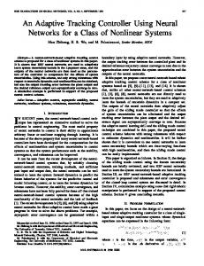
some types of radial basis function (RBF) networks [5], [19], [23], a class of fuzzy if–then systems [15], learning vector quantization (LVQ) classifiers [11], [12], [14], edited nearest neighbor rules [6], fuzzy nearest neighbor rules [1], [13], [26], multiple prototype classifiers [2], and a number of neuralnetwork implementations of the nearest neighbor design [7], [17], [26]. Each of these has specific strategies and algorithms for finding the prototypes. The diagram in Fig. 1 groups the GNPC’s into presupervised and postsupervised designs with respect to the way the prototypes are found and labeled. In each group we distinguish GNPC’s with crisp and noncrisp (soft) labels for the prototypes. The connection between models and groups of models that fit within the GNPC framework has been addressed many times [3], [20]. Ripley [20] points out that some neural network models are just renamed kernel or Parzen classifiers. Asymptotically (when the number of prototypes/hidden nodes tends to infinity) the models coincide. Here we are interested in the finite-sample case; then different designs can offer significantly different performance. We study two semiparametric designs (one from each GNPC group) and show that presupervised mixture modeling needs one type of assumption (decomposition) while the dual postsupervised design needs two types of assumption (decomposition and homogeniety) for optimality relative to the standard Bayes error rate (Bayes-optimality [8], p. 16). Two RBF networks are chosen as representatives: the RBF trained by orthogonal least squares (OLS RBF) [4], a presupervised GNPC; and the RBF trained by clustering followed by nonnegative least squares (NNLS RBF) [19], a postsupervised GNPC. Section II gives our definition of the GNPC. In Sections III and IV we define the mixture models and derive conditions for Bayes-optimality of the GNPC. Experimental results with OLS RBF and NNLS RBF on two data sets (one synthetic and one real) are given in Section V. Section VI contains our conclusions.

II. THE GENERALIZED NEAREST PROTOTYPE CLASSIFIER (GNPC) mutually exclusive classes with crisp labels , where is the canonical basis of . Objects associated with class are labeled by the vector if , and , otherwise. be the feature space. Any function is Let be a called a crisp classifier. Let set of point-prototypes. Our GNPC is based on the following principles. We consider

1045–9227/99$10.00  1999 IEEE

KUNHCEVA AND BEZDEK: PRESUPERVISED AND POSTSUPERVISED PROTOTYPE

1143

Fig. 1. Families of generalized nearest prototype classifiers.

• Every prototype may “vote” for all classes, and the is defined by strength of ’s vote for class . a constant • The closer (more similar) is to the prototype , the higher the “relevance” of the -th vote is to the label for . Assume that each prototype is labeled by a column vector , thereby constituting a label . In our model the number matrix may be less than, equal to, or greater than of prototypes may be the number of classes ; and the label vector crisp or soft (fuzzy, probabilistic, possibilistic). Definition 1: A norm-induced similarity function , where is a set of parameters for , is of any monotonically decreasing function on . For example, if denotes the any norm metric Euclidean norm metric, could be (1)

Let be an aggregation function defined as generalized matrix multiplication using an operator instead of summation and a operator instead of multiplication. Let and be two matrices of size and , respectively. The matrix is defined as (2) Definition 2: The GNPC is implemented with the 5-tuple where is the set of prototypes; • • is the label matrix for the prototypes in classes; is a similarity function, where is a set • of parameters; is any -norm and is an aggregation operator [24]. • , the GNPC calculates the For an unlabeled vector between and vector of similarities

1144

IEEE TRANSACTIONS ON NEURAL NETWORKS, VOL. 10, NO. 5, SEPTEMBER 1999

which is then used to compute the label vector . As a special case the crisp to if GNPC assigns the crisp class label (3) Ties are broken randomly. Thus any unlabeled is labeled on the basis of its proximity combined with their class (or similarity) to the prototypes label information. Note that the GNPC at (3) assigns a crisp class label. The GNPC is completely specified by and . We can try different combinations of these GNPC choices and select the most successful GNPC design by optimizing its classification accuracy. In the next section we derive two models of the GNPC based on postsupervised and presupervised mixture modeling [18], [21] where the components are kernel-type functions (e.g., Gaussians). Each component corresponds to a prototype whose probability density function (PDF) gives the similarity of to the prototype . The mixing coefficients are used to compute the “soft” class labels of the prototypes. III. POSTSUPERVISED GNPC DESIGN Let be a random vector coming from one of classes. Let denote the prior probability; the the posterior probability class-conditional PDF; and . Let be the unconditional PDF for class (4)

(prototypes) as possible, so the approximation at (6) will differ from the true value at (4). We call (6) the decomposition assumption, and shall refer to it as (A1). We require that the mixture components of (6) have kernel-type PDF’s. That is, besides the condition (7) is based on a kernel-type function [10], , where is a is a prototype. A typical smoothing parameter and choice is the Gaussian kernel

each

(8) is a covariance matrix. Often is chosen to be where the same for all prototypes, or at least common for all the prototypes of each class. Equation (6) provides Parzen’s estimate of the PDF at (4) [8], [10] if each kernel is centered at a data point and if the number of data points approaches infinity. In the sequel we assume that we have a satisfactory algorithm to estimate all the parameters of the mixture (6), , and the the a priori probabilities for the classes . We do not restrict the conditional probabilities . The classes and the hidden class-conditional PDF’s categories are related through

The objective is to build a GNPC that produces a Bayesoptimal classification decision (assuming a zero-one loss mawhen trix), i.e., the class label assigned to is (5) Hence, a sufficient condition for optimality of the GNPC is have the same order that, if sorted by magnitude, . as the sorted We consider mixture modeling for the GNPC design. Mixture modeling is used to identify the priors, the classconditional PDF’s and the unconditional PDF, which can . Kernel be used with Bayes rule to calculate mixture models are nonparametric. Typically, all training data points are used, each one generating a kernel (e.g., Parzen’s window classifier). Other methods (e.g., neural networks) try to reduce the number of kernels without much degradation in classification performance. Shrinking the number of kernels shifts the mixture paradigm from nonparametric toward “semiparametric” [23]. can be approximated by another We assume that using as priors mixture of new PDF’s (A1)

(9) is the probability of class if hidden category where occurs. By conditioning (9) on we obtain the posterior probability for class as (10) To build an RBF network Traven [23] assumes that (A2)

(11)

We call (11) the homogeneity assumption and shall refer to it as (A2). Substituting (11) into (10) (12) Developing (12) further, we have with Bayes rule (13)

(6) Let

will be referred to as “hidden catewhere gories” [23]. We will try to use as few mixture components

(14)

KUNHCEVA AND BEZDEK: PRESUPERVISED AND POSTSUPERVISED PROTOTYPE

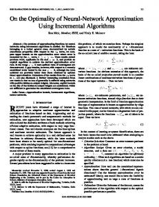
Fig. 2. Scatter plot of

X

disregarding the class labels.

1145

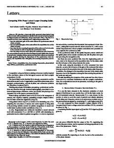
Fig. 3. Case X

:

x

p(

j i)

A:

= p ^(x

The j Ci ); i

most

desirable

class

labeling

of

= 1 ; 2.

Dropping the denominator of (13), which is the same for all , and dividing by , the Bayes-optimal classifier under assumptions (A1) and (A2) can be represented by the following set of discriminant functions: (15) is the probability of simultaneous occurrence where . Assuming kernel-type of class and hidden category can be represented as , PDF’s, is any where is a similarity function (Definition 1) and . Equation (15) can then be rewritten as norm on

(16) stands for the probability . Therefore, the where postsupervised GNPC that is a Bayes-optimal classifier under assumptions (A1) and (A2) is

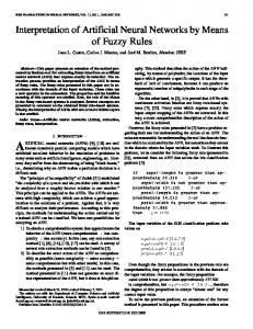
Fig. 4. Case B: The worst class labeling of

X

:

p(

x j 1) = p(x j 2).

different labelings corresponding to “ideal” sampling from the respective cases. Case A: Ideally, the classes will correspond one-to-one to the hidden categories (e.g., Fig. 3, where class 1, denoted by , and class 2, denoted circles has the same parameters as by filled circles, has the same parameters as ). In this case if otherwise (18)

product average The following examples illustrate the situation with respect . Plotted in Fig. 2 is data set to Bayes optimality of GNPC consisting of 200 two-dimensional (2-D) points. The vectors . come from two classes with labels was The class labels of the points are not shown in Fig. 2. generated from (4) using a mixture of two Gaussians with identity covariance matrices, viz., (17) and are the prototypes of the where and ). two mixture components (hidden categories Below we detail four cases A, B, C, and D. The illustrations with (Figs. 3, 4, 5, 7, and 9) use the same data set

is proportional to , it is Since easy to show that the classification decision of GNPC is Bayes-optimal. is Case B: The worst possible case of class labeling of shown in Fig. 4. The classes are equiprobable and the classconditional PDF’s are identical, i.e., these labels correspond to the case where (19) and cannot be In this case the hidden categories associated with a specific class label. Therefore, it is pointless and because the probability to attempt to identify of each class to occur together in either category is 0.5. will be 0.5, and, again, this The error of the GNPC is the Bayes-optimal error rate. The situation in Fig. 4 can occur when some other feature has been used to label the data and this information is not represented in the current feature . space Case C: Fig. 5 shows the case where each class has a bimodal PDF whose modes are situated at the common proand . Class-conditional PDF’s that will generate totypes

1146

IEEE TRANSACTIONS ON NEURAL NETWORKS, VOL. 10, NO. 5, SEPTEMBER 1999

Fig. 5. Case C: Decomposable bimodal class-conditional PDF’s.

Fig. 7. Case D: Nondecomposable class-conditional PDF’s.

is built as suggested above. Here the homogeneity assumption (A2) is not satisfied. The class labels in Fig. 7 are artificially assigned to (Fig. 2) according to the rule: is assigned to ; Class 1, if Class 2, otherwise. For this labeling the class-conditional PDF’s are shown in (22) and (23) at the bottom of the page, where Fig. 6. Case C: Bimodal class-conditional PDF’s for x

2