Neural Networks Prediction of Soil Hydraulic Functions ... - Groundwater

Neural Networks Prediction of Soil Hydraulic Functions for Alluvial Soils Using Multistep Outflow Data B. Minasny, J. W. Hopmans,* T. Harter, S. O. Eching, A. Tuli, and M. A. Denton ABSTRACT

monly used soil-water retention model is the one introduced by van Genuchten (1980):

Indirect methods for prediction of soil hydraulic properties play an important role in understanding site-specific unsaturated water flow and transport processes, usually via numerical simulation models. Specifically, pedotransfer functions (PTFs) to predict soil-water retention have been widely developed. However, few datasets that include unsaturated hydraulic conductivity data are available for prediction purposes. Moreover, those available employ a variety of measurement techniques. We show that prediction of soil-water retention and unsaturated hydraulic conductivity curves from basic soil properties can be improved if hydraulic data are determined by a single measurement method that is consistently applied to all soil samples. Here, we present a unique dataset that consists of 310 soil-water retention and unsaturated hydraulic conductivity functions, all of which were obtained from the multistep outflow method. With this dataset, neural networks coupled with bootstrap aggregation were used to predict the soilwater retention and hydraulic conductivity characteristics from basic soil properties, that is, sand, silt, and clay content, bulk density (␳b), saturated water content, and saturated hydraulic conductivity. The prediction errors of water content were about 3 to 4% by volume. Unsaturated hydraulic conductivity predictions improved significantly when a so-called performance-based algorithm was utilized to minimize residuals of soil hydraulic data rather than hydraulic parameters. The root mean squared of residuals for predicted values of water content and unsaturated hydraulic conductivity were reduced by about 50% when compared with predicted hydraulic functions using a published neural networks program Rosetta. Results from a sensitivity analysis suggest that the hydraulic parameters are mostly sensitive to sand content and saturated water content.

␪(h) ⫽ ␪r ⫹

␪s ⫺ ␪r , m (1 ⫹ |␣h|n)

[1]

where ␪(h) denotes the volumetric water content (L3 L⫺3) at the corresponding soil-water matric head h (L), ␪r and ␪s are the residual and saturated water content, ␣ is a scaling parameter (L⫺1), n is a curve shape factor (⫺), and m is an empirical constant that can be related to n, or m ⫽ 1 ⫺ 1/n. When substituted into the unsaturated hydraulic conductivity (K) model of Mualem (1976), the unsaturated hydraulic conductivity is described by: K(Se) ⫽ KoS el [1 ⫺ (1 ⫺ S e1/m)m]2,

[2]

where Se denotes the normalized water content, Se ⫽ (␪ ⫺ ␪r)/(␪s ⫺ ␪r), l is a pore geometry parameter, and Ko is a matched saturated hydraulic conductivity (L T⫺1), extrapolated from fitted unsaturated K values. This fitted value for Ko is usually smaller than the true saturated conductivity, Ks, since the latter is largely controlled by soil structural elements, such as cracks and macropores. Therefore, Ko is usually considered a fitting parameter (van Genuchten and Nielsen, 1985). Soil hydraulic properties, typically measured for small core samples with a length scale of 10⫺1 m or smaller, vary greatly in space (Nielsen et al., 1973). Consequently, a large number of samples is needed to characterize fields with length scales of 102 m or larger. However, measurement of soil hydraulic properties is generally difficult, time consuming, and expensive, so that few complete datasets are available. Therefore, indirect methods have been pursued that predict soil hydraulic properties from more easily measured soil parameters. An excellent review of indirect methods, including the application of neural networks, is presented by Leij et al. (2002). Wo¨sten (1990) postulated that the use of these indirect methods is acceptable as long as it includes the uncertainty of the estimations. Specifically, the use of PTFs was introduced by Bouma (1989). These are predictive functions of certain soil properties estimated from other simpler and routinelymeasured soil properties that are generally available (McBratney et al., 2002). The application of PTFs to predict soil-water retention using basic soil properties such as sand, silt, and clay content, and ␳b is now commonly used in soil science studies because predictions of either water content at a specific soil-water matric potential or water retention parameters (Schaap et al., 1998) have been quite successful (Romano and Palla-

T

he dynamic simulation of soil hydrological processes is increasingly being used to predict the unsaturated soil-water regime in environmental applications and in crop yield modeling to study agronomic management practices. Models that simulate unsaturated water flow in soil have been widely developed and adopted. Essential to their application is the availability of unsaturated soil hydraulic properties, that is, the soil-water retention and unsaturated hydraulic conductivity functions. The soil hydraulic properties are usually represented by a parametric model. Although many of these have been developed (Kosugi et al., 2002), the most comB. Minasny, Faculty of Agriculture, Food, and Natural Resources, McMillan Building A05, The Univ. of Sydney, NSW 2006, Australia; J.W. Hopmans, T. Harter, and M.A. Denton, Hydrology Program, Dep. of Land, Air, and Water Resources, 123 Veihmeyer Hall, Univ. of California, Davis, CA 95616; S.O. Eching, Dep. of Water Resources, Water Use Efficiency Office, 901 P Street, Third Floor, P.O. Box 942836, Sacramento, CA 94236-0001; A. Tuli, Dep. of Environmental Sci., 2217 Geology Building, Univ. of California, Riverside, CA 92521. Received 12 June 2003. *Corresponding author ([email protected]).

Abbreviations: ␳b, bulk density; MR, mean residual; OM, organic matter; PTF, pedotransfer function; RMSR, root mean squares of residual.

Published in Soil Sci. Soc. Am. J. 68:417–429 (2004).  Soil Science Society of America 677 S. Segoe Rd., Madison, WI 53711 USA

417

418

SOIL SCI. SOC. AM. J., VOL. 68, MARCH–APRIL 2004

dino, 2002). Also the saturated hydraulic conductivity can be predicted reasonably well from such basic soil properties. Models such as Mualem’s Eq. [2] are subsequently used to predict the unsaturated hydraulic conductivity from water retention data. However, more accurate unsaturated conductivity functions are expected if these are predicted directly from measured K values, for example, by neural network analysis. Only few studies show the application of PTFs to predict unsaturated hydraulic conductivity data from basic soil properties. Among those are Bloemen (1980) in the Netherlands, who correlated parameters of the Brooks-Corey function to soil texture and organic matter (OM) content. Similar techniques were applied by Gonc¸alves et al. (1997) in Portugal, Jaynes and Tyler (1984) for glacial till soil in the USA, and Vereecken (1995) in Belgium using alternative analytical expressions for the K(h) function. Among the first to use neural networks to predict K was Tamari et al. (1996), who included horizon designation, soil textural class, OM content, ␳b, and water content at specific soil-water matric potential values as input variables. Wo¨sten et al. (1999) extracted data from the European soil hydraulic database to derive van Genuchten function parameters using sand, silt, and clay content, soil ␳b, and organic carbon content. Schaap and Leij (2000) predicted parameters l and Ko from sand, silt, and clay content, and ␳b using neural network analysis. The latter study concluded that K-predictions were improved if soil-water retention function parameters were included as input parameters. The performance of different published PTFs in predicting K(h) for selected German soils was evaluated by Wagner et al. (2001). Among the main issues that limit the accurate prediction of unsaturated hydraulic conductivity is the lack of a soil hydraulic database that includes measured unsaturated conductivity data. Public domain databases such as UNSODA (Nemes et al., 2001) do provide both hydraulic properties and basic soil physical data from different parts of the world for various soil types. However, the unsaturated hydraulic conductivity values that are included in these data sets are generally obtained by many different measurement techniques. Typically, these methods are limited by specific assumptions and apply to relatively narrow water content ranges, so that K-prediction results are expected to depend on measurement type (Mallants et al., 1997). Although the measurement type effect applies to prediction of soil-water retention data as well, its effect may not be as consequential, because the predicted ␪ range of the retention curve is much smaller than the predicted unsaturated K range. Thus, when PTFs are used to predict soil hydraulic data, uniformity of measurement methods is desirable. Specifically, Schaap and Leij (1998) showed that the PTF prediction depended on the training data set, whereas the accuracy was largely controlled by data quality. It is expected that improved prediction accuracies will be obtained when a training data set is used with soil hydraulic and related physical properties that are determined from similar measurement techniques.

In this paper, we examine the simultaneous prediction of soil-water retention and unsaturated hydraulic conductivity from soil hydraulic data that were estimated with the multistep outflow method (Eching et al., 1994b), whereby the soil hydraulic parameters of Eq. [1] and [2] are estimated with an inverse modeling technique. Characteristically, this measurement technique provides estimated soil hydraulic parameters from the matching of experimental observations of transient water flow with numerical modeling results. The presented measured data span 310 soil samples, largely from three different datasets, representing a variety of alluvial soils and soil textures across three different regions in the California San Joaquin Valley. The main objective of the presented analysis is to show that neural network prediction of both soil-water retention and unsaturated hydraulic conductivity will improve if all analyzed data are obtained by identical measurement methods. MATERIALS AND METHODS Multistep Outflow Method Many laboratory and field methods exist to determine the highly nonlinear soil hydraulic functions of the vadose zone, represented by soil-water retention and unsaturated hydraulic conductivity curves. Most methods are either static (soil-water retention) or steady state (unsaturated hydraulic conductivity), and consequently, measurements are usually time-consuming and limited to the wet water content range. The multistep outflow method applies inverse modeling for indirect estimation of both water retention and hydraulic conductivity curves in a single transient drainage experiment. The multistep outflow method has become an attractive method for estimating soil hydraulic properties (Crescimanno and Iovino, 1995; Vereecken et al., 1997). The outflow method originates from the one-step outflow experiment of Gardner (1956). Kool et al. (1985) formulated the inverse solution for the one-step pressure outflow experiment using a numerical solution of transient water flow, that is, Richards’ equation, with the van Genuchten model of Eq. [1] and [2] representing the soil hydraulic properties. Starting with initial parameter estimates, a numerical model solution computes the theoretical drainage outflow rate of an initiallysaturated soil sample. Parameters of the soil hydraulic functions are updated iteratively in an optimization routine, thereby continuously reducing the residuals until a predetermined convergence criterion (reduction in objective function value between two consecutive iterations) is achieved. Kool et al. (1985) successfully applied the inverse method to estimate ␪r, ␣, and n from cumulative outflow measurements. Van Dam et al. (1994) proposed the multistep outflow method, by increasing the air pressure in multiple smaller steps. Their results showed that the outflow data from a multistep experiment provided sufficient information to yield a unique solution. Alternatively, Eching et al. (1994b) demonstrated that unique solutions were obtained if the multistep outflow method was combined with automated soil-water matric head measurements of the draining soil core. A comprehensive review of inverse modeling for estimation of soil hydraulic properties, including one-step and multistep methods was presented by Hopmans et al. (2002). Although relatively complex, inverse modeling can provide quick results. As an additional advantage, inverse modeling for soil hydrau-

MINASNY ET AL.: PREDICTION OF SOIL HYDRAULIC FUNCTIONS

lic characterization allows the simultaneous estimation of both the soil-water retention and unsaturated hydraulic conductivity function from a single transient experiment. The inverse method mandates combination of experimentation with numerical modeling, thus requiring both accurate experimental procedures and advanced numerical modeling and optimization algorithms. Since the optimized hydraulic functions are mostly needed as input to numerical flow and transport models for prediction purposes, it has the added advantage that the hydraulic parameters are estimated by similar numerical models. In addition, the parameter optimization procedure provides a confidence interval of the optimized parameters, although their interpretation may be misleading. Some caution must be exercised when applying the multistep outflow method. First, laboratory measurements, although accurate, provide hydraulic information for a relatively small soil core, detached from its surroundings. Moreover, as is the case for any method, the parameter estimates are only valid for the range of the experimental conditions, and care must be exercised in their extrapolation. Finally, inverse problems for parameter estimation of soil hydraulic functions can be ill posed because of experimental design, measurement, and model errors.

Training Dataset The presented 310 soil hydraulic data were collected from three different field projects. The first dataset consists of 144 undisturbed soil samples that were collected from seventy two 64- by 64-m plots at two depths (25 and 50 cm) in a 40-ha field (Tuli et al., 2001a). This Long Term Research on Agricultural Systems (LTRAS) project was conducted at the Russell Ranch of the University of California near Davis, CA, to study the long-term effects of irrigation and nitrate application to the sustainability of California agriculture. The field includes three different soil series: the Yolo (fine-silty, mixed, superactive, nonacid, thermic Mollic Xerofluvents), the Rincon (fine smectitic, thermic Mollic Haploxeralfs), and the Brentwood (fine, smectitic, thermic Typic Haploxerepts). Within each 64- by 64-m plot, 8.25-cm i.d. and 6-cm-long soil cores were collected with a soil core sampler. The range of values of the main soil physical properties as obtained from these soil cores were: ␳b, 1.22 to 1.66 g cm⫺3; OM, 0.43 to 1.63%; saturated hydraulic conductivity, 0.0002 to 17.7900 cm h⫺1; saturated water content, 0.32 to 0.50 cm3 cm⫺3; sand (50–2000 ␮m), 11 to 56%; silt (2–50 ␮m), 34 to 80%; and clay (⬍2 ␮m), 3 to 22%. The second data set consists of 88 soil cores collected from a 32-ha furrow-irrigated field (Diener) on the west side of the San Joaquin Valley (Eching et al., 1994a), near Five Points, CA. The soil is of the Panoche series (fine-loamy, mixed, superactive, thermic Typic Haplocambids), having very deep and well-drained uniform profiles with a wide range of textures. Soil texture varied from a silty loam and sandy clay loam on the south east side of the field to a loamy sand and sandy loam with patches of silty clay, clay loam, and silty clay in the rest of the field. Undisturbed soil cores were taken from the 0.3- and 0.6-m soil depth at 44 locations, uniformly distributed within the irrigated field. The range of values of the main soil physical properties as obtained from these soil cores were: ␳b, 1.26 to 1.87 g cm⫺3; OM, 0.03 to 0.18%; saturated water content, 0.32 to 0.54 cm3 cm⫺3; sand, 13 to 99%; silt, 1 to 76%; and clay, 1 to 15%. No saturated hydraulic conductivity data were available for the Diener dataset. Extracted core locations in the field were grouped into clays (6 locations), loams (12 locations), and sands (26 locations). The third data set consists of 69 sediment cores. Of the three data sets, this is the only data set representing unsaturated sediments below the root zone. The core samples represent

419

unsaturated sediments in their native, anthropogenically unaltered depositional environment. Continuous cores were extracted with a Geoprobe Systems (Salina, KS) direct push drill rig. A Geoprobe Macrocore sampler (5.2-cm o.d.) containing a PVC liner (3.8-cm i.d.) was driven in 1.2-m intervals through unsaturated sediments to a depth of ⬎15 m. Sediment cores were obtained from 18 locations spaced 3 to 12 m apart within a 1-ha orchard at the Kearney Field Station (Parlier) in the San Joaquin Valley, CA. The location overlies the near-distal part of the Kings River alluvial fan emanating from the Kings River watershed at the foot of the generally granitic Sierra Nevada mountain range. The continuous cores were cut in 10-cm long core sections that were fitted within PVC and aluminum sleeves to fit a 5.1-cm i.d. Tempe pressure cell (Tuli et al., 2001b). The range of values of the main soil physical properties as obtained from these soil cores were: ␳b, 1.26 to 1.87 g cm⫺3; OM, 0.01 to 0.20%; saturated water content, 0.22 to 0.47 cm3 cm⫺3; saturated hydraulic conductivity, 0.002 to 30.0 cm h⫺1; sand, 13 to 98%; silt, 1 to 76%; and clay, 1 to 17%. Five major textural units were distinguished in the cores: sand, loamy sand, sandy loam, silt/silt loam/loam/silty clay loam, clay loam/clay, and variably thick hardpan at the 3- to 5-m depth. A former alluvial channel bed of limited width and consisting of clean medium sand was encountered at the 7- to 10-m depth. Nine additional soil data were included from Eching et al. (1994b) and Corwin et al. (2003). For each core sample, soil properties and hydraulic functions were determined with the following procedure. Upon saturation, the soil cores were placed on a screen to measure the saturated hydraulic conductivity (Ks) with the constant head method (Klute and Dirksen, 1986). After completion of the saturated hydraulic conductivity measurement, the samples were assembled in Tempe pressure cells for estimation of soil-water retention and unsaturated hydraulic conductivity function using the multistep outflow method. The samples were resaturated with the 0.01 M CaCl2 solution by wetting through a bottom porous membrane assembly. For Datasets 1 and 2, the bottom plate consisted of a 1-bar ceramic plate. For the third dataset, the bottom assembly included a thin porous nylon membrane with low hydraulic resistance (Hopmans et al., 2002). A positive air pressure was applied to the top of the cell, while cumulative water outflow is automatically recorded from a pressure transducer that was installed in the bottom of a burette. The soil-water matric head inside the draining soil core was simultaneously measured with a miniature tensiometer connected to a pressure transducer. The multistep pressure increments were determined by soil texture, but maximum air pressures did generally not exceed 600 cm. The air pressure was increased when the cumulative outflow curve approached a plateau value, indicating nearhydraulic equilibrium. With the transient soil-water matric head and cumulative drainage data, the parameters of the soil-water retention and unsaturated hydraulic conductivity functions were estimated from the inverse solution of the Richards’ equation as presented in Eching et al. (1994b) and Hopmans et al. (2002). During the optimization, ␪s was fixed to its measured value whereas the soil tortuosity-connectivity parameter, l, was assumed to be 0.5. Therefore, the optimized parameters were ␪r, ␣, n, and Ko. The final dataset includes weight percentages of sand, silt, and clay content, and field dry ␳b as determined from standard methods (Klute and Dirksen, 1986), measured ␪s and Ks, and optimized van Genuchten parameters ␪r, ␣, n, and Ko. The statistics of the complete dataset are given in Table 1, whereas the soil textural distribution is presented in Fig. 1. The textural range of the combined sample set is dominated by sands to silt loams. The multistep outflow method is typi-

420

SOIL SCI. SOC. AM. J., VOL. 68, MARCH–APRIL 2004

Table 1. Statistics of the complete training dataset.† Variables

Units

Sand content % weight Silt content % weight Clay content % weight Bulk density (␳b) g cm⫺3 Residual water content (␪r) cm3 cm⫺3 Saturated water content (␪s) cm3 cm⫺3 Scalding parameter (␣) cm⫺1 Curve shape factor (n ) – log10(K0)‡ log10 (cm h⫺1) log10 (cm h⫺1) log10(Ks)§

Average SD 46 41 13 1.51 0.17 0.39 0.019 2.048 ⫺0.68 ⫺0.21

Min.

Max.

23.6 6 100 20.3 0 80 7.3 0 55 0.14 1.13 1.87 0.11 0.00 0.42 0.06 0.22 0.55 0.018 0.001 0.124 1.063 1.057 7.641 0.99 ⫺3.40 2.00 0.87 ⫺3.77 1.86

† Number of samples, Ns ⫽ 310, except for log(Ks), for which Ns ⫽ 219. ‡ Ko, matched saturated hydraulic conductivity. § Ks, saturated hydraulic conductivity.

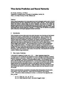
cally not suitable for soil hydraulic property measurement of clayey soils because the maximum applied pressure step will generally not exceed 600 to 700 cm. The texture triangle shows the textural differences between the three data. The LTRAS samples are dominantly silty loam and loamy soils. The sampled Kearney soils are low in clay content, whereas the Diener samples consist mainly of loamy and sandy loam soils. For the neural network analysis, soil-water retention and unsaturated hydraulic conductivity data were extracted from the set of hydraulic functions (Fig. 2a,b) at discrete matric pressure head values: 0, 40, 60, 80, 200, 400, and 600 cm. The textural differences between the three datasets are readily apparent in Fig. 2. Specifically, the finer-textured soil materials of the LTRAS site have high soil-water retention, while the Kearney soils with their low clay content have the smallest water retention and highest hydraulic conductivity.

Neural Network Analysis In the past decade, artificial neural networks have become an alternative method for the prediction of soil properties (Pachepsky et al., 1996; Schaap et al., 1998). A neural network is modeled after the functioning of the nervous system. Through a complex mathematical structure of interconnecting layers, knowledge is acquired through a learning process by

which interneuron connection strengths (weights) are used to store knowledge (Ripley, 1996). The feed-forward neural networks that is applied in this study consists of a set of input units, x, representing the input variables, and a set of output units, y, representing the output variables, interconnected by hidden units, z. Each set of the three types of units are arranged in layers. The mathematical model consists of a set of operations or network that is presented in Eq. [3]. First, an input vector x is multiplied by weighting factors that are assembled in array W, resulting in the hidden unit vector z. In a second step, this vector z is passed to a layer containing the activation or transfer function, f, which produces r. Finally, in the third step, the target vector y is computed from a linear combination of r, with the weighting factors in array U, or:

zj ⫽

Ni

兺 wjl xl ⫹ wj0,

rj ⫽ f(zj), yk ⫽

j ⫽ 1, ..., Nh

l⫽1 Nh

兺 ukj rj ⫹ uk0,

j⫽1

j ⫽ 1, ..., Nh k ⫽ 1, ..., No

[3]

where Ni, Nh, and No denote the number of input variables, hidden units, and number of output variables, respectively. The bias values wj0 and uk0 provide for offsets for zj and yk, respectively. The transfer function is usually a sigmoidal function that is selected such that it accommodates the nonlinearity of the specific input–output relationship. The function that is commonly used is the hyperbolic tangent, or

f(zj) ⫽ tanh(zj) ⫽ 1 ⫺

2 1 ⫹ exp(2zj)

[4]

The advantage of neural networks is that they can be used to predict one or more output types through a flexible network of weights, transfer functions, and input variables without a priori assuming a specific relationship between input and output and without making specific assumptions about the statistical distribution of input or output variables. Instead, the network is trained on a training dataset to find the relationship between input and output by optimizing the weighting factors in arrays W and U in Eq. [3] through minimization of the differences between measured and predicted output variables. Once the weights of the neural network have been determined, it can be used for prediction of output from input variables other than the training set. Neural networks also have significant disadvantages that must be taken into consideration. First, their interpretation is often difficult and subjective, as the fitting with the transfer function is a black-box approach. Second, as is usually the case in optimization, the sets of optimized weighting factors are not necessarily mathematically unique because of the likelihood of convergence at local minima. Consequently, different initial weight values may yield different neural network results that deviate from the global minimum. To avoid nonuniqueness of the final solution, many network predictions can be obtained from multiple realizations of the input dataset by the bootstrap technique, also known as bagging (Breiman, 1996).

Neural Network Training of Soil Hydraulic Parameters

Fig. 1. Particle size distribution of the training dataset. To determine soil type, find intersection of lines, parallel to main coordinate axes.

The objective of the presented study is to train the neural network so that the parameter vector p ⫽ [␪r, ␪s, ␣, n, K0] can be predicted from a basic soil property vector x that includes soil texture, ␳b, saturated water content, and saturated hydrau-

MINASNY ET AL.: PREDICTION OF SOIL HYDRAULIC FUNCTIONS

421

Fig. 2. (a) Soil-water retention, and (b) unsaturated hydraulic conductivity curves of the training dataset, making distinction between Long Term Research on Agricultural Systems (LTRAS), Kearney, and Diener datasets. ␪, water content; h, soil-water matric head; K, hydraulic conductivity.

lic conductivity. Conventionally, this is done by optimization of the neural network weights so that the objective function that includes the sum of squares of the residuals between the measured and predicted parameters is minimized, or

O(W,U) ⫽

Ns

No

兺兺

i⫽1 k⫽1

[pˆik (xi) ⫺ pik]2,

[5]

where Ns denotes the number of samples, No is the number of output parameters, and pˆ (x) is the output vector with the predicted parameters, as determined from the input vector x. Because the parameters in p are highly nonlinear and correlated, thus possibly nonidentifiable, a fitted parameter set does not warrant an equally good prediction of soil hydraulic data. Therefore, for estimation of the soil-water retention curves, Minasny and McBratney (2002a) proposed an alternative objective function for training neural networks to predict the van Genuchten parameters from the basic input data. Instead of minimizing the hydraulic parameters, the objective function operates on the residuals of the measured and predicted soilwater retention data, that is, ␪(h ) data pairs. They called this the Neuro-m method, which was referred to by Romano and Palladino (2002) as having a performance-based objective function. The Neuro-m method is extended in this study to simultaneously predict water retention and unsaturated hydraulic conductivity, with the following objective function:

O(W,U) ⫽

[␪ˆ is (xi, his, pi) ⫺ ␪is (his)]2 ⫹ ␴2 (␪) i⫽1 s⫽1 ˆ is (xi, his, pi) ⫺ log Kis (his)]2 [log K , [6] ␴2 (log K) Ns Nd(i)

兺 兺

where Nd(i ) defines the number of water retention and conductivity data at corresponding soil-water matric head values

ˆ (x,h,p) denote the of soil sample i, and ␪ˆ (x,h,p) and log K predicted water content and unsaturated hydraulic conductivity values at matric head h with the fitted parameter vector p, calculated via the neural network from the input vector x. Reciprocal values of the variance, ␴2, of the respective measurements are used as weights to account for differences in magnitude between ␪ and log K. Equation [6] was minimized with a modified version of the Levenberg-Marquardt method. Values of K were log-transformed because K is generally found to be log-normal distributed (Schaap and Leij, 2000), so that they were computed from Eq. [2] to yield

log[K(Se)] ⫽ log(Ko) ⫹ l log(Se) ⫹ 2 log[1 ⫺ (1 ⫺ Se1/m)m]

[7]

where Se is computed from the corresponding h value. For all unsaturated hydraulic conductivity functions, l was fixed to 0.5. Log transformations of K, ␣, and n ⫺ 1 ensured that their back-transformed values were positive and that n ⬎ 1. The neural network consisted of a single hidden layer. We conducted a trial to determine the appropriate number of hidden units by training the data with a range of hidden units (Minasny and McBratney, 2002a). From this trial, we concluded that predictions did not improve significantly by use of more than six hidden units. Four different neural network models were trained to test the ability of various input parameter combinations (Table 2) to predict p. These input combinations represent a hierarchical structure of data availability (Schaap et al., 1998). The least amount of input was needed for the first training set that included particle size distribution data only (Ni ⫽ 3). The other three training sets also included input parameters: ␳b (Ni ⫽ 4), ␳b and ␪s (Ni ⫽ 5), and ␳b with ␪s and log Ks (Ni ⫽ 6). The training was conducted by first minimizing the standard objective function of Eq. [5]. All the input and output values

422

SOIL SCI. SOC. AM. J., VOL. 68, MARCH–APRIL 2004

Table 2. Hierarchical set of input variables for training neural networks. No. 3 4 5 6

Types of input variables for vector x Sand, Sand, Sand, Sand,

silt, silt, silt, silt,

and and and and

clay clay clay clay

content content, and bulk density (␳b) content, ␳b, and saturated water content (␪s) content, ␳b, and ␪s, and log10(Ks)†

† Ks, saturated hydraulic conductivity.

were scaled to zero-mean and unit-variance so that the different magnitudes of the parameters did not affect optimization. The optimized weights after 20 iterations were used as initial estimates for the performance-based optimization, minimizing Eq. [6]. With Nh ⫽ 6 and Ni ⫽ 4, the weighting matrix W consists of 6-by-5 elements, including the six bias values. If five hydraulic parameters are optimized (No ⫽ 5), the weighting matrix U consists of 5-by-7 elements (including the five bias values). The neural network training algorithm was implemented in the Neuroman program (Minasny and McBratney, 2002b).

Bagging Recent empirical evidence suggests that combining different neural networks can enhance the prediction accuracy (Perrone and Cooper, 1993). With use of bootstrap aggregating or bagging (Breiman, 1996), one can generate many different data sets from a single original data set to fit different neural network models. These networks are then combined to form a single aggregated predictor. The bootstrap method (Efron and Tibshirani, 1993) was developed to assess the accuracy of a prediction by generating different prediction models from different realizations of the training dataset. Dane et al. (1986) used bootstrapping to provide confidence intervals for the statistical distribution of soil ␳b and to determine the minimum sample size needed to estimate the mean with a specified degree of precision. Bootstrapping assumes that the training data set is a representation of the population and that multiple realizations from the population can be simulated from this single dataset. This is done by repeated sampling with replacement from the original dataset, D, of size N to obtain B bootstrap data sets, each of size N. Therefore, each bootstrap data set contains different data. Since the neural net is trained for each realization, the bagging procedure produces B neural networks. Each bootstrap dataset Db, b ⫽ 1, 2, …, B, yields a prediction model, yˆ b(x), where y either represents a vector with predicted parameter (parameter-based) or ␪ and log(K ) (performance-based) values. The bagging estimate is calculated from the mean of all B model predictions, or

yˆ bag(x) ⫽

1 B

B

兺

yˆ b(x),

[8]

b⫽1

whereas the uncertainty of the model was calculated from its standard deviation. Schaap et al. (1998) applied a similar bootstrap procedure for their neural network model for predicting soil-water retention function parameters. Bagging is especially useful when analyzing highly variable data sets. The aggregated predictor averages the prediction across all bootstrap samples, thereby reducing the prediction variance. The prediction accuracy increases if the prediction method is unstable; that is, small changes in the training data of the bootstrap can result in large changes in the resulting predictor (Breiman, 1996). The size B of the bagged or bootstrap aggregated predictor used was 50; that is, data were resampled 50 times, thus produc-

ing 50 neural networks. For each neural net, the van Genuchten parameters were predicted, and ␪(h ) and K(h ) data pairs for each soil sample were calculated. The mean and 95% confidence interval of the predicted hydraulic parameters, water retention, and hydraulic conductivity data were computed by all B predicted data pairs, Eq. [8]. Finally, predicted soil hydraulic parameters were determined by fitting the Mualemvan Genuchten function (Eq. [1] and [2]) to the mean predicted water retention and hydraulic conductivity data. This algorithm was implemented in a program called Neuro Multistep, which is available upon request.

Performance Measure The performance of the neural network was evaluated from values of the mean residual (MR) and root mean square residual. The MR is a measure of prediction bias, with negative and positive MR-values indicating underestimation and overprediction, respectively. It is defined by

MR ⫽

1 N

N

兺 (yˆ i ⫺ yi),

[9]

i⫽1

where N is equal to Ns ⫻ Nd, and yˆ and y represent predicted and measured ␪ or log K values, respectively, at the seven different matric head values for each of the 310 soil samples (N ⫽ 7 ⫻ 310). The root mean square of residuals (RMSRs) defines the expected magnitude of the prediction error, or

RMSR ⫽

冤N1 兺 (yˆ ⫺ y ) 冥 N

1/2

i

i

2

.

[10]

i⫽1

For soil-water content, the units of MR and RMSR are cm3 cm⫺3, while for conductivity the units are dimensionless because the subtraction of two logarithmic K values is equal to the logarithm of their ratio. Our prediction results were compared with those obtained by the neural network program Rosetta of Schaap et al. (2001). Briefly, Rosetta estimates soil-water retention parameters ␪r, ␪s, ␣, and n with a training data set of soils from the temperate and subtropical regions in Europe and the USA. Their unsaturated hydraulic conductivity parameters, Ko and l, were predicted separately by the UNSODA database.

RESULTS AND DISCUSSION Performance of Neuro Multistep The performance of Neuro Multistep, predicting soil hydraulic properties from the 310 sample training dataset is shown in Table 3. In addition to the performancebased optimization (Eq. [6]) proposed in this paper, we also conducted the standard parameter-based optimization (Eq. [5]) using software JMP version 5.0 (SAS Institute, 2002). Training the neural network with the performance-based objective function provided better predictive capability than with the standard parameterbased optimization. The prediction bias was also lower. Differences are most evident for the conductivity predictions. Specifically, the RMSR value of log(K) was reduced by a factor of two, and the bias was more than one order of magnitude smaller, when compared with the parameter-based optimizations. Furthermore, adding more input parameters than texture only slightly improved the prediction of conductivity with the parameter-based approach.

423

MINASNY ET AL.: PREDICTION OF SOIL HYDRAULIC FUNCTIONS

Table 3. Statistics of neural networks prediction of water retention and hydraulic conductivity with different combinations of input variables.†

In part, we believe that the lesser performance of the parameter-based approach is caused by the inherent assumption that hydraulic parameters are independent, whereas many studies have demonstrated that water retention and unsaturated hydraulic conductivity data are determined by the correlated set of hydraulic parameters. Therefore, an accurate prediction of one or more hydraulic parameters does not guarantee a good fit of both the water retention and hydraulic conductivity data. The performance-based optimization ensures that the predicted parameters fit both water retention and unsaturated conductivity data rather than only the hydraulic parameters. The difference in performance between the two approaches can also be attributed to the nonuniqueness or nonidentifiability of the hydraulic models. In the latter case, one may wonder whether the soil hydraulic data can be fit by more than a single parameter set. The differences between the parameterbased (pˆ par) and performance-based optimizations (pˆ per) for three different soil samples (silt loam from LTRAS, sand from Kearney, and sandy loam from Diener) of the training data set are highlighted in Table 4. While parameter-based optimization gives closer values of n, Ko, and similar RMSR values for water retention, the RMSR values for log(K) are generally much higher, as expected from using Eq. [10] as the performance criterium. Predicted soil hydraulic properties with performancebased optimization are relatively unbiased, as concluded from the near-zero value of the MR of both ␪ (retention data) and log(K) (unsaturated hydraulic conductivity). The RMSR for ␪ is approximately 4% moisture content, whereas the RMSR for log(K) is about one order of magnitude. Increasing the number of relevant input variables to include ␳b and ␪s improved the prediction, particularly of log(K). The predicted soil-water content data are compared with their measured values in Fig. 3a. Whereas most ␪ data are concentrated near the 1:1 line across the whole water content range, some Kearney data (triangles) were underpredicted. The predicted unsaturated hydraulic conductivity values (Fig. 3b) matched their corresponding measured values except for a small number of low hydraulic conductivity values of the LTRAS samples (diamonds). As the results of Table 3 show, incorporating measured Ks values as an additional input param-

MR ␪

Inputs cm Parameter-based optimization Sand, silt, clay‡ Sand, silt, clay, ␳b‡ Sand, silt, clay, ␳b, ␪s‡ Sand, silt, clay, ␳b, ␪s, log(Ks)§ Performance-based optimization Sand, silt, clay‡ Sand, silt, clay, ␳b‡ Sand, silt, clay, ␳b, ␪s‡ Sand, silt, clay, ␳b, ␪s, log(Ks)§ Rosetta Sand, silt, clay, ␳b‡ ␪r, ␪s, ␣, n‡

3

RMSR

cm⫺3

⫺0.0142 ⫺0.0133 ⫺0.0076 ⫺0.0115

␪

log10(K ) cm 0.2592 0.2311 0.2377 0.2231

3

log10(K )

cm⫺3

0.047 0.043 0.039 0.034

1.328 1.356 1.383 1.370

0.0007 0.0002 0.0001 0.0030

⫺0.013 ⫺0.015 ⫺0.016 ⫺0.044

0.042 0.038 0.034 0.035

1.065 0.919 0.888 0.733

⫺0.0515 –

0.546 0.225

0.073 –

1.978 1.212

† ␪s, saturated water content; ␳b, bulk density; Ks, saturated hydraulic conductivity; MR, mean residual; Ns, number of samples; Nd, number of water retention and conductivity data; RMSR, root mean squares of residuals. ‡ Number of data (Ns ⫻ Nd) ⫽ 2170. § Number of data (Ns ⫻ Nd) ⫽ 1533.

eter, improves the prediction of unsaturated hydraulic conductivity only slightly, while increasing the bias of both ␪ and log(K).This indicates that Ks has little meaning for unsaturated K, which is better defined by Ko. The bagging procedure yielded 50 different W and U matrices for each set of input parameters. When predicting soil hydraulic data for soils other than the training data set, these same weighting arrays are used to obtain 50 soil hydraulic functions, from which the mean and confidence limits are computed. Three examples of neural network predictions for the same soil samples as in Table 4 are presented in Fig. 4. Figure 4a presents the predicted ␪(h) and K(h) functions with 95% confidence intervals for a LTRAS sample with a sand and clay content of 21 and 18%, respectively, and ␳b, ␪s, and Ks values of 1.5 g cm⫺3, 0.41 cm3 cm⫺3, and 0.08 cm h⫺1, respectively. For the second sample, a sand from Kearney in Fig. 4b, the sand and clay content, ␳b, ␪s, and Ks values are 98 and 2%, 1.46 g cm⫺3, 0.37 cm3 cm⫺3, and 60 cm h⫺1, respectively. Finally, Fig. 4c presents the predicted curves and confidence intervals for a Diener sample with sand and clay content of 43 and 14%, and ␳b and ␪s values of 1.53 g cm⫺3 and 0.4 cm3 cm⫺3, respectively. As expected, all predicted hydraulic data fall within the confidence bands. In this example, the predic-

Table 4. Comparison of true with predicted parameters and their respective root mean squares of residual (RMSR) values with the parameter-based (pˆpar) and performance-based (pˆper) optimizations for three soils of the training data set. Silt loam LTRAS† Parameter‡ ␪r ␪s ␣ n log(Ko) RMSR ␪ RMSR log(K )

Sand Kearney

Loam Diener

p

pˆpar

pˆper

p

pˆpar

pˆper

p

pˆpar

pˆper

0.326 0.410 0.015 1.694 ⫺1.854

0.237 0.409 0.011 1.563 ⫺1.530 0.027 0.651

0.234 0.409 0.011 1.667 ⫺1.700 0.014 0.490

0.045 0.367 0.036 4.674 1.380

0.071 0.370 0.037 3.628 1.284 0.031 1.767

0.000 0.371 0.032 4.479 1.097 0.069 0.560

0.119 0.400 0.013 1.413 ⫺0.928

0.198 0.406 0.017 1.581 ⫺0.874 0.006 0.279

0.129 0.398 0.013 1.714 ⫺1.129 0.031 0.280

† LTRAS, long term research of agricultural systems. ‡ ␣, scaling parameter; ␪, volumetric water content; ␪r, residual water content; ␪s, saturated water content; K, hydraulic conductivity; Ko, matched saturated hydraulic conductivity; n, curve shape factor.

424

SOIL SCI. SOC. AM. J., VOL. 68, MARCH–APRIL 2004

Fig. 3. Measured vs. predicted (a) water retention and (b) unsaturated hydraulic conductivity data when five input parameters are used (sand, silt, clay, bulk density, and saturated water content). ␪, water content; K, hydraulic conductivity.

tion of the Kearney sand is quite uncertain as reflected by the high confidence interval and large RMSR values, which demonstrates the lower prediction capability for sand. Generally, all conductivity predictions show that the prediction uncertainty is larger as the unsaturated hydraulic conductivity decreases with decreasing matric potential values.

Comparison with Other PTFs A key measure of the predictability performance of neural networks is the RMSR value. Literature values for RMSR of soil-water retention data range from 0.02 to 0.10 cm3 cm⫺3 (Wo¨sten et al., 2001, Table 2). The RMSR values of Neuro Multistep with the training data of multistep outflow data are equal or better than reported elsewhere. Since studies reporting on K predictions are limited, a comparison with only few studies can be made. Specifically, Schaap and Leij (2000) reported an average RMSR value of log(K) of 1.18, using percentages of sand, silt, and clay, and ␳b as input parameters. This value was reduced to 0.84 when K was predicted from the soil-water retention parameters ␪r, ␪s, ␣, and n. The average RMSR value of the study of Zhuang et al. (2001) was 1.24. The RMSR of log(K) of our training data set is of similar magnitude or lower than either reported study. In comparing the presented predictions with other studies, we must note that our study predicts the water retention and unsaturated conductivity simultaneously from the same input data, while most other training data sets apply neural networks to water retention and unsaturated hydraulic conductivity separately. To determine the influence of the training data set

on the prediction, we applied the Rosetta neural networks of Schaap et al. (2001) to our training dataset. The RMSR values with Rosetta (Table 3) were about twice as large. The larger prediction error by Rosetta is a consequence of two factors. First, it demonstrates the value of the training data set, that is, our data set includes hydraulic data for Californian alluvial soils only, whereas the Rosetta training data set consists of a much wider range of soils across the globe. Second, we hypothesize that the higher prediction accuracy of Neuro Multistep is caused by the mere fact that all soilwater retention and unsaturated hydraulic conductivity data were determined by the multistep outflow method in the same laboratory. As also pointed out by Vereecken (2002), the evaluation of prediction methods for unsaturated hydraulic conductivity must consider the number and type of measurement methods that were used. Because of the limited number of soil types that were used in the training data set of Neuro Multistep, one must be careful in extrapolating our results to soils with larger values of clay content than included here. To further investigate the usefulness of the prediction of neural networks to specific textural groups, we separated the training data set into two main soil textural groups: sands (sand, loamy sand, and sandy loam) and loams (loam, silt loam, sandy clay loam, clay loam, and silty clay loam), each with about an equal number of soil samples. The distribution of RMSR for both textural groups as well as for all textures combined is presented in Fig. 5a (retention) and Fig. 5b (unsaturated conductivity). This is done for Neuro Multistep with all four input data sets of Table 3, as well as for Rosetta with percentages of sand, silt, and clay, and ␳b. Each box plot

Fig. 4. Examples of measured (dots) and predicted (solid line) soil hydraulic functions with five input parameters. The dashed lines span the 95% confidence interval of the predictions. The comparison is presented for (a) Long Term Research on Agricultural Systems (LTRAS) silt loam, (b) Kearney sand, and (c) Diener loam. ␪, water content; h, soil-water matric head; K, hydraulic conductivity; RMSR, root mean squares of residuals.

Fig. 5. Box plots of RMSR values for different neural network models predicting (a) water retention, and (b) unsaturated hydraulic conductivity. The box plots summarize the distribution of root mean squares of residuals (RMSR). The horizontal line in each box signifies the median value, whereas top and bottom of the box represent the 25th and 75th quantiles. The whiskers extend from the ends of the box to the outermost data point that falls within the distances of upper quartile ⫹ 1.5 (interquartile range), and lower quartile ⫺ 1.5 (interquartile range), respectively. ␪, water content; K, hydraulic conductivity.

MINASNY ET AL.: PREDICTION OF SOIL HYDRAULIC FUNCTIONS

Table 5. Values of root mean squares of residual (RMSR) for predicted matched saturated hydraulic conductivity (Ko) with different combinations of input variables with the training data set grouped in sandy and loamy soils. RMSR log10(Ko) Inputs† Neuro Multistep Sand, silt, clay‡ Sand, silt, clay, ␳b‡ Sand, silt, clay, ␳b, ␪s‡ Sand, silt, clay, ␳b, ␪s, log(Ks)§ Rosetta Sand, silt, clay, ␳b‡ ␪r, ␪s, ␣, n‡

Sands

Loams

All

0.621 0.579 0.594 0.572

0.829 0.813 0.800 0.706

0.806 0.788 0.777 0.693

1.391 1.011

1.014 0.966

1.062 0.968

† ␣, scaling parameter; ␪r, residual water content; ␪s, saturated water content; ␳b, bulk density; Ks, saturated hydraulic conductivity. ‡ Number of samples Ns for sands ⫽ 35, loams ⫽ 273, All ⫽ 310. § Number of samples Ns for sands ⫽ 24, loams ⫽ 195, All ⫽ 219.

presents the median (center line) and the 25 and 75% percentiles (top and bottom) with the cross lines representing the median. Notably, the prediction error is larger for the sandy soil group than for the loamy group. We presume that the difference in prediction error is attributed to the high nonlinearity of the coarser soil group. However, it can be noted that opposite results were obtained with Rosetta, with lower RMSR values for sandy soils than loamy soils. This may be because of the better representation of sandy soil materials in the training dataset of Rosetta (Schaap et al., 2001). Table 5 compares prediction results of Neuro Multistep with Rosetta for Ko only, with the same sets of input parameters as Table 3, making distinction between the sandy and loamy soil groups. In contrast to the unsaturated hydraulic data, the prediction error of Ko for sands is smaller than for the loamy soil group. It is hypothesized that the smaller prediction error is caused by the smaller measurement error of the saturated hydraulic conductivity of sandy soils. It is also noted that the Ko prediction is largely improved by including the measured saturated hydraulic conductivity, Ks, as input variable. This would suggest a two-step approach. In the first step one predicts Ko, which would be subsequently used in the second step to improve the unsaturated hydraulic conductivity predictions.

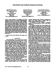
Sensitivity Analysis Finally, it is interesting to determine the sensitivity of the various input parameters on the predicted soil hydraulic parameters. Figure 6 shows the prediction profile (SAS Institute, 2002) of five input variables on parameters: ␪r, ␪s, ␣, n, and log(K0), and water retention at a matric head value of ⫺100 cm: ␪⫺100. The input and output parameters are normalized by their respective mean (␮) and standard deviation (␴) as follows: x* ⫽ (x ⫺ ␮)/␴.

[11]

The sensitivity plot in Fig. 6 depicts the predicted response of the hydraulic parameters when changing each input variable across a wide range of values, as determined by its minimum and maximum value. These

427

ranges are indicated on the x axis for each input variable. For each input variable, its value is varied while all other input variables are held constant to their respective mean values. The vertical dotted lines represent the mean values for each input parameter, whereas the horizontal dotted lines indicate the corresponding predicted values. The plot shows that the response of the outputs is not a linear function of the input variables, particularly ␣ and n, which is also because of log transformation in the prediction. Sand content seems to influence most of the parameters. An increase in both sand and silt content leads to a decrease in values of ␪r, ␪s, and ␣, and increase in the values of n and Ko. The influence of clay content on prediction of water content at a matric head of ⫺100 cm (␪⫺100) appears to be relatively small compared with the other input variables, implying that the change in clay content will not affect the prediction of ␪. This may be the result of the low clay content of the soil used in the training data set. The value of ␪⫺100 is influenced by the combination of all input variables. Saturated water content, ␪s, appears to be another important input variable, having more influence on the parameter predictions than ␳b. A change in ␪s value affects all parameters. It should be noted that the plot only shows the sensitivity at specific values, whereas interactions between all input variables are expected. The use of neural networks enables incorporation of the nonlinearities and interactions between the input and output variables.

CONCLUSIONS The results confirm our initial hypothesis that the consistency of the data set plays important role in calibrating PTFs. We have compiled a unique data set of soil-water retention and unsaturated hydraulic conductivity functions that were simultaneously estimated (measured) with the multistep outflow method. With this unique dataset, we successfully developed PTFs that simultaneously predict water retention and hydraulic conductivity by neural network analysis. We note that the predictions in this paper can only be used for the range of soil textures that were included in the training data set (sands and loams). Moreover, the predicted hydraulic properties pertain to the experimental measurement range of soil-water matric heads between 0 and ⫺600 cm only. The neural networks model developed in this paper has not been validated on an independent dataset. Currently, we developed the model with all available data to maximize its predictive capabilities. Additional data for other soil types and geographic regions will have to be included in the training dataset, thereby providing a more general applicable prediction. However, we doubt that a single PTF can be found that provides equal and accurate predictions for every soil and geographic region in the world as what was presented here. The neural networks analysis in this paper is implemented in a program called Neuro Multistep. The program can be obtained by contacting either Dr. Budiman Minasny ([email protected]) or Dr. Jan W. Hopmans ([email protected]), or can be downloaded

428

SOIL SCI. SOC. AM. J., VOL. 68, MARCH–APRIL 2004

Fig. 6. Sensitivity analysis of various input data (horizontal axis) to soil hydraulic parameters (vertical axis). ␪⫺100, water retention at a matric head value of ⫺100 cm; ␪r, residual water content; ␪s, saturated water content; ␳b, bulk density; K, hydraulic conductivity.

from the University of Sydney website: http://www.usyd. edu.au/su/agric/acpa/software (verified 19 Nov. 2003). REFERENCES Bloemen, G.W. 1980. Calculation of hydraulic conductivities from texture and organic matter content. Z. Pflanzenernaehr. Bodenk. 143:581–605. Bouma, J. 1989. Using soil survey data for quantitative land evaluation. Adv. Soil Sci. 9:177–213. Breiman, L. 1996. Bagging predictors. Mach. Learn. 24:123–140. Corwin, D.L., S.R. Kaffka, J.D. Oster, J.W. Hopmans, Y. Mori, J.W. van Groenigen, C. van Kessel, and S.M. Lesch. 2003. Assessment and field-scale mapping of soil quality properties of a saline-sodic soils. Geoderma 114:231–259. Crescimanno, G., and M. Iovino. 1995. Parameter estimation by inverse method based on one-step and multi-step outflow experiments. Geoderma 68:257–277. Dane, J.W., R.B. Reed, and J.W. Hopmans. 1986. Estimating soil parameters and sample size by bootstrapping. Soil Sci. Soc. Am. J. 50:283–287. Eching, S.O., J.W. Hopmans, and W.W. Wallender. 1994a. Estimation

of in situ unsaturated sol hydraulic functions from scaled cumulative drainage data. Water Resour. Res. 30:2387–2394. Eching, S.O., J.W. Hopmans, and O. Wendroth. 1994b. Unsaturated hydraulic conductivity from transient multi-step outflow and soil water pressure data. Soil Sci. Soc. Am. J. 58:687–695. Efron, B., and R.J. Tibshirani. 1993. An introduction to the bootstrap. Monogr. 57 on Statistics and Applied Probability. Chapman & Hall, London. Gardner, W.R. 1956. Calculation of capillary conductivity from pressure plate outflow data. Soil Sci. Soc. Am. Proc. 20:317–320. Gonc¸alves, M.C., L.S. Pereira, and F.J. Leij. 1997. Pedo-transfer functions for estimating unsaturated hydraulic properties of Portugese soils. Eur. J. Soil Sci. 48:387–400. Hopmans, J.W., J. Simunek J., N. Romano, and W. Durner. 2002. Water retention and storage: Inverse methods. p. 963–1004. In J.H. Dane and G.C. Topp (ed.) Methods of soil analysis: Part 4—Physical methods. SSSA Book Series No. 5. SSSA, Madison, WI. Jaynes, D.B., and E.J. Tyler. 1984. Using soil physical properties to estimate hydraulic conductivity. Soil Sci. 138:298–305. Klute, A., and A. Dirksen. 1986. Hydraulic conductivity and diffusivity: Laboratory methods. p. 687–734. In A. Klute (ed.) Methods of soil analysis. Part I. 2nd ed. Physical and mineralogical methods. Agron. Monograph No. 9. ASA, CSSA, and SSSA, Madison, WI.

MINASNY ET AL.: PREDICTION OF SOIL HYDRAULIC FUNCTIONS

Kool, J.B., J.C. Parker, and M.Th. van Genuchten. 1985. Determining soil hydraulic properties for one-step outflow experiments by parameter estimation. I. Theory and numerical studies. Soil Sci. Soc. Am. J. 49:1348–1354. Kosugi, K., J.W. Hopmans, and J.H. Dane. 2002. Water retention and storage: Parametric models. p. 739–757. In J.H. Dane and G.C. Topp (ed.) Methods of soil analysis: Part 4—Physical methods. SSSA Book Ser. No. 5. SSSA, Madison, WI. Leij, F., M.G. Schaap, and L.M. Arya. 2002. Water retention and storage: Indirect methods. p. 1009–1045. In J.H. Dane and G.C. Topp (ed.) Methods of soil analysis: Part 4—Physical methods. SSSA Book Ser. No. 5. SSSA, Madison, WI. Mallants, D., D. Jacques, P.-H. Tseng, M.Th. van Genuchten, and J. Feyen. 1997. Comparison of three hydraulic property measurement methods. J. Hydrol. (Amsterdam) 199:295–318. McBratney, A.B., B. Minasny, S.R. Cattle, and R.W. Vervoort. 2002. From pedotransfer function to soil inference system. Geoderma 109:41–73. Minasny, B., and A.B. McBratney. 2002a. The neuro-m method for fitting neural network parametric pedotransfer functions. Soil Sci. Soc. Am. J. 66:352–361. Minasny, B., and A.B. McBratney. 2002b. Neuroman: Neural networks program for generating parametric pedotransfer functions. Available at: http://www.usyd.edu.au/su/agric/acpa/software (verified 18 Nov. 2003). Australian Centre of Precision Agriculture, the Univ. of Sydney, NSW, Australia. Mualem, Y. 1976. A new model for predicting the hydraulic conductivity of unsaturated porous media. Water Resour. Res. 12:513–522. Nemes, A., M.G. Schaap, F.J. Leij, and J.H.M. Wo¨sten. 2001. Description of the unsaturated soil hydraulic database UNSODA version 2.0. J. Hydrol. (Amsterdam) 251:151–162. Nielsen, D.R., J.W. Biggar, and K.T. Erh. 1973. Spatial variability of field measured soil water properties. Hilgardia 42:215–259. Pachepsky, Y.A., D.J. Timlin, and G. Varallyay. 1996. Artificial neural networks to estimate soil water retention from easily measurable data. Soil Sci. Soc. Am. J. 60:727–773. Perrone, M.P., and L.N. Cooper. 1993. When networks disagree: Ensemble methods for neural networks. p. 126–142. In R.J. Mammone (ed.) Neural networks for speech and image processing. ChapmanHall, New York. Ripley, B.D. 1996. Pattern recognition and neural networks. Cambridge Univ. Press, Cambridge. Romano, N., and M. Palladino. 2002. Prediction of soil water retention using soil physical data and terrain attributes. J. Hydrol. (Amsterdam) 265:56–75. SAS Institute. 2002. JMP statistics and graphics guide. v. 5. SAS Inst., Cary, NC. Schaap, M.G., and F.L. Leij. 1998. Database-related accuracy and uncertainty of pedotransfer functions. Soil Sci. 10:765–779. Schaap, M.G., and F.L. Leij. 2000. Improved prediction of unsaturated hydraulic conductivity with the Mualem-van Genuchten model. Soil Sci. Soc. Am. J. 64:843–851.

429

Schaap, M.G., F.L. Leij, and M.Th. Van Genuchten. 1998. Neural network analysis for hierarchical prediction of soil hydraulic properties. Soil Sci. Soc. Am. J. 62:847–855. Schaap, M.G., F.L. Leij, and M.Th. Van Genuchten. 2001. Rosetta: A computer program for estimating soil hydraulic parameters with hierarchical pedotransfer functions. J. Hydrol. (Amsterdam) 251: 163–176. Tamari, S., J.H.M. Wo¨sten, and J.C. Ruiz-Sua´rez. 1996. Testing an artificial neural network for predicting soil hydraulic conductivity. Soil Sci. Soc. Am. J. 60:1732–1741. Tuli, A., M.A. Denton, J.W. Hopmans, T. Harter, and J.L. MacIntyre. 2001b. Multi-step outflow experiment: From soil preparation to parameter estimation. Land, Air and Water Resources Rep. No. 100037. Univ. of California, Davis. Tuli, A., K. Kosugi, and J.W. Hopmans. 2001a. Simultaneous scaling of soil water retention and unsaturated hydraulic conductivity functions assuming lognormal pore-size distribution. Adv. Water Resour. 245:677–688. van Dam, J.C., J.N.M. Stricker, and P. Droogers. 1994. Inverse method for determining soil hydraulic functions from multi-step outflow experiments. Soil Sci. Soc. Am. J. 58:647–652. van Genuchten, M.Th. 1980. A closed-form equation for predicting the hydraulic conductivity of unsaturated soils. Soil Sci. Soc. Am. J. 44:892–898. van Genuchten, M.Th., and D.R. Nielsen. 1985. On describing and predicting the hydraulic properties of unsaturated soils. Ann. Geophys. 3:615–628. Vereecken, H. 1995. Estimating the unsaturated hydraulic conductivity from theoretical models using simple soil properties. Geoderma 65:81–92. Vereecken, H. 2002. Comment on the paper, “Evaluation of pedotransfer functions for unsaturated soil hydraulic conductivity using an independent data set.” Geoderma 108:145–147. Vereecken, H., R. Kaiser, M. Dust, and T. Pu¨tz. 1997. Evaluation of the multistep outflow method for the determination of unsaturated hydraulic properties of soils. Soil Sci. 162:618–631. Wagner, B., V.R. Tarnawski, V. Hennings, U. Mu¨ller, G. Wessolek, and R. Plagge. 2001. Evaluation of pedo-transfer functions for unsaturated soil hydraulic conductivity using an independent data set. Geoderma 102:275–297. Wo¨sten, J.H.M. 1990. Use of soil survey data to improve simulation of water movement in soils. Ph.D. thesis. Univ. of Wageningen, the Netherlands. Wo¨sten, J.H.M., A. Lilly, A. Nemes, and C. Le Bas. 1999. Development and use of a database of hydraulic properties of European soils. Geoderma 90:169–185. Wo¨sten, J.H.M., Y.A. Pachepsky, and W.J. Rawls. 2001. Pedotransfer functions: Bridging gap betwen available basic soil data and missing soil hydraulic characteristics. J. Hydrol. (Amsterdam) 251:123–150. Zhuang, J., K. Nakayama, G.R. Yu, and T. Miyazaki. 2001. Predicting unsaturated hydraulic conductivity of soil based on some basic soil properties. Soil Till. Res. 59:143–154.