avoid getting stuck in a local minimum, and produce a global minimum as T â 0. ... by the largest positive eigenvalue of w (Peterson and Söderberg, 1989) (see also ..... the total length of a closed tour connecting a set of N cities with given ...
LU TP 02-30
Neural Optimization Carsten Peterson and Bo S¨oderberg Complex Systems Division, Dept. of Theoretical Physics, Lund University To appear in The Handbook of Brain Theory and Neural Networks, (2nd edition), M.A. Arbib (ed.), Bradford Books/The MIT Press.
Introduction Many combinatorial optimization problems require a more or less exhaustive search to achieve exact solutions, with a computational effort growing exponentially or worse with system size. Hence, for large problems, the quest for an exact solution has to be abandoned. Instead, various kinds of heuristic methods have been developed to yield reasonably good approximate solutions. Artificial neural network (ANN) methods in general fall within this category, and particularly interesting in the context of optimization are recurrent network methods based on deterministic annealing. In contrast to most other methods, these are not based on a direct exploration of the given discrete state-space; instead, they utilize an interpolating continuous (analog) space, allowing for shortcuts to good solutions. Key concepts here are the mean-field (MF) approximation (Hopfield and Tank, 1985; Peterson and S¨oderberg, 1989) and annealing. While early versions were confined to problems encodable with a quadratic energy in terms of a set of binary variables, the method has in the last decade been extended to deal with more general problem types, both in terms of variable types and energy functions, and has evolved to a general-purpose heuristic for combinatorial optimization. An appealing feature is that the basic MF dynamics is directly implementable in VLSI (see ANALOG VLSI IMPLEMENTATIONS OF NEURAL NETWORKS), facilitating hardware implementations.
Recurrent Networks Recurrent networks appear in the context of associative memories (Hopfield, 1982) as well as difficult optimization problems (Hopfield and Tank, 1985; Peterson and S¨oderberg, 1989). Such networks resemble statistical models of magnetic systems (“spin glasses”), with an atomic spin state (up or down) seen as analogous to the “firing” state of a neuron (on or off). This similarity has been the source of much inspiration for neural network studies. The archetype of a recurrent network is the Hopfield model (Hopfield, 1982), based on
1
an energy function of the form E(s) = −
1X wij si sj 2 ij
(1)
in terms of binary variables (or Ising spins, as used in magnetic models), si =±1 (in some contexts, equivalent 0, 1-spins are preferred), with symmetric weights wij . Due to the identity s2i = 1, diagonal components wii are redundant and can be assumed to vanish. With an appropriate choice of weights determined by a set of stored patterns, the latter appear as local minima, satisfying
si = sgn
X
wij sj .
(2)
j
With a simple asynchronous dynamics based on iterating Equation 2, this system turns into a recurrent ANN, having the local minima as stationary points; in effect this model serves as an associative memory (see COMPUTING WITH ATTRACTORS).
Update Modes Note the importance of asynchronous update (in random order or sequentially), in which case E(s) is a Lyapunov function, and cannot increase – this guarantees the convergence towards a fixed point defining a local energy minimum. Attempting to iterate Equation 2 in synchrony would not necessarily yield convergence to a local minimum – the system may wind up in a two-cycle instead, with a subset of the spins flipping signs in every update. This behavior can be understood by viewing two consecutive synchronous updates of the N spins as a single sequential update of a system of 2N spins, {xi , yi }, where first the P x are updated based on y (as xi = sgn j wij yj ), and then the y based on the new x. The ˆ y) = − P xi wij yj is a Lyapunov function, and the extended corresponding energy E(x, ij system must converge to a fixed point (x∗ , y ∗ ). If x∗ and y ∗ are equal, they define a fixed point s∗ (a local energy minimum) of the original system; otherwise a two-cycle results with s alternating between x∗ and y ∗ . If x∗ and y ∗ are maximally different (x∗ = −y ∗ ), they define two equivalent local maxima of E. Other, mixed cases can be seen as saddle points. Consider also the related problem of minimizing −E (i.e. maximizing E), obtained by flipping all signs in w. In terms of x, y, the corresponding update equations differ from the original only by replacing, say, y by −y. Thus, there is a one-to-one correspondence between sequences of states for s obtained for −E and for E: One is obtained from the other by flipping the signs of every second state. This shows that with synchronous update, the system cannot really tell the difference between minimizing and maximizing E. The undesirable behaviour of synchronous update can be avoided by introducing stabilizing self-couplings in the form of positive diagonal elements large enough to make w a positive-definite matrix (and E(s) a concave function); this, however, has the negative side-effect of adding a multitude of stationary states that are not local minima. Below, sequential update mode without self-couplings will be assumed where not otherwise stated.
2
Optimization with Recurrent Networks Many types of optimization problems can be encoded in terms of a Hopfield model, with the energy function adapted to a specific problem by a dedicated choice of weights, such that global minima of E(s) correspond to solutions. For simple problems, the recurrent network dynamics of iterating Equation 2 can be used to find a solution. For more difficult problems, however, the system will most likely get trapped in a non-optimal local minimum close to the starting point, which is not desired. A more refined approach is needed to reach the global minimum or at least a low-lying local minimum.
Stochastic Methods A possible strategy is to employ a stochastic algorithm that allows for uphill moves, such as Simulated Annealing (SA) (see SIMULATED ANNEALING AND BOLTZMANN MACHINES). There, a stochastic neighborhood search method is used in an attempt to generate a sequence of configurations distributed according to a Boltzmann distribution, P (s) ∝ e−E(s)/T , where T is an artificial temperature representing the noise level of the system, which is slowly decreased (annealing). With a very slow annealing rate, the system can avoid getting stuck in a local minimum, and produce a global minimum as T → 0. Such a procedure can be very CPU consuming, however.
The Mean-Field Equations An alternative is given by MF annealing, where the stochastic SA method is approximated by a deterministic dynamics based on the MF approximation, defined as follows for a system of Ising spins. The true Boltzmann distribution P (s) is approximated by the direct product of singleQ spin distributions, i pi (si ). Such a factorized distribution is characterized by the absence of correlations between the spins, and is completely determined by the single-spin averages vi ≡ hsi i = pi (1) − pi (−1) ∈ [−1, 1]. The parameters vi are variationally determined so as to minimize the free energy, F (v) = E(v) − T S(v), (3) P
P
where E(v) ≡ hE(s)i ≡ − 21 i6=j ωij vi vj is the average energy, while S(v) ≡ − 12 i [(1 + vi ) log(1 + vi ) + (1 − vi ) log(1 − vi )] is the entropy associated with the approximating distribution. Minimization of F with respect to vi directly yields the MF equations, vi = tanh(ui /T ), with ∂E(v) X ui ≡ − ≡ wij vj ∂vi j
(4) (5)
The analog MF variables vi take values in the interval [−1, 1], interpolating between the discrete spin states ±1 – which is natural since they approximate the thermal spin averages hsi iT .
3
Analog Network The MF equations (4) can be solved by asynchronous iteration, in analogy with the discrete Equation 2, the only difference being the replacement of the sharp step function sgn(ui ) by a smooth sigmoid tanh(ui /T ), with an adjustable parameter 1/T controlling the gain: High T corresponds to very smooth sigmoids, while in the low-T limit the stepfunction of Equation 2 is recovered. Most of the discussion on update modes in the context of Equation 2 applies also to the MF dynamics; thus, with asynchronous updating, the free energy F (v) of Equation 3 defines a Lyapunov function guaranteeing the convergence to a fixed point defined by a local minimum of F .
Mean-Field Annealing In MF (or deterministic) annealing, the fixed-T MF dynamics is slowly modified by lowering an initially high T , using e.g. a geometric annealing schedule. For the quadratic Hopfield energy, the dynamics then will exhibit a behavior with two phases: At large temperatures, the system relaxes to a trivial fixed point v o , with vio = 0. As the temperature sinks below a critical value Tc , v o becomes unstable and non-trivial fixed points emerge; as T → 0 these are pushed towards discrete (±1) values, representing a specific decision made as to the solution of the problem in question. The position of the bifurcation point Tc can be determined by linearizing Equation 4 around v o , i.e. replacing the sigmoid function (tanh) by its argument. With sequential updating without self-couplings, this yields a smooth tangent bifurcation at a temperature given by the largest positive eigenvalue of w (Peterson and S¨oderberg, 1989) (see also DYNAMICS AND BIFURCATIONS IN NEURAL NETS). For an energy without the exact symmetry under v → −v, as results e.g. by adding a linear energy term, a distinct bifurcation might be absent; then the high-T fixed point is only approximately zero, with the MF variables evolving continuously from smaller to larger values over a finite T interval. This is no problem: A suitable initial T can still be estimated. Alternatively, an auxiliary spin variable can be introduced and multiplied to the linear term to restore symmetry. Deterministic annealing yields a more efficient method for finding low-lying energy minima than setting T = 0 from the start (i.e. iterating Equation 2). Tracking a local minimum as T is lowered can guide the system to better low-T minima (see STATISTICAL MECHANICS OF NEURAL NETWORKS).
The Graph Bisection Problem As an example application illustrating the above abstract discussions we will use Graph Bisection (GB): A graph with an even number N of nodes is to be divided into two halves of N/2 nodes each, such that the cut-size (the number of connections between the halves) is minimal (Figure 1 A). The encoding is particularly transparent here because of the binary nature of the problem: With each node i a binary spin si is associated, to be assigned a value ±1 representing whether the node will wind up in the left or right partition of Figure
4
A
B
Figure 1: A, a graph bisection problem; B, a K = 4 graph partition problem. 1A. The graph is given in terms of a symmetric connection matrix J, such that an element Jij equals 1 if vertices i, j are connected, and 0 if not (or if i = j). With this notation, the product Jij si sj is nonzero only for a connected pair of nodes i, j, yielding 1 if they are put P in the same partition and -1 if not. Thus, the cut-size is proportional to −1/2 ij Jij si sj plus an unimportant constant. In addition, one needs to take into account the global constraint of equal partition of P the nodes, requiring i si = 0. This can be done by adding to the energy function a term P that penalizes an illegitimate partition. A term proportional to ( si )2 will obviously do the trick. P Discarding the constant diagonal part i s2i = N , we obtain a Hopfield energy function, Equation 1, with wij = Jij − α (1 − δij ): E=−
1X 2
à !2 X X α Jij si sj + si − s2i
ij
2
i
(6)
i
where the constraint coefficient α sets the relative strength of the penalty term. Equation 6 has a structure common in combinatorial optimization problems: E = Cost + Global constraint. The origin of the difficulty inherent in this kind of problem is very transparent here: The conflict associated with minimizing the two competing terms makes the system frustrated, which often leads to the appearance of many local minima. For large random GB problems, MF annealing yields a distinctively better performance than simple iteration of Equation 2.
Recurrent Potts Networks For GB and many other optimization problems, an encoding in terms of binary elementary variables is natural. However, there are many problems where the natural elementary decisions are of the type one-of-K with K > 2. Early attempts to approach such problems with recurrent network methods were based on neuron multiplexing (Hopfield and Tank, 1985), where for each elementary K-fold decision, a set of K binary 0/1-neurons was used, with a syntax constraint requiring that
5
precisely one of them be on (i.e. = 1) implemented in a soft way with a penalty term. In the original work on the traveling salesman problem, as well as in subsequent investigations on the graph partition problem (Peterson and S¨oderberg, 1989), this approach did not yield high-quality solutions in a parameter-robust way. A more efficient encoding is based on K-state Potts spins with the syntax constraint built in. This confines the dynamics to the relevant parts of solution space, and leads to a drastically improved performance.
MF Annealing with Potts Spins A K-state Potts spin is a variable that has K possible values (states). For our purposes, the best representation is in terms of a K-dimensional vector s = (s1 , s2 , . . . , sK ), with the ath state given by the ath principal unit vector, defined by sa = 1, sb = 0 for b 6= a. These vectors point to the corners of a regular K-simplex (see Figure 2 for the case of K = 3). They are all normalized and mutually orthogonal, and fulfill in addition the P syntax constraint a sa = 1.
vi3
vi2 vi1 Figure 2: The cubic solution space corresponding to the neuron multiplexing encoding for K = 3, interpolating between the eight allowed spin states at the corners of the cube. With a Potts encoding the solution space is restricted to the shaded triangle, interpolating between the three allowed Potts spin states at its corners. The MF equations for a system of Potts spins si with a given energy function E(s) in multilinear form (∂ 2 E/∂sia ∂sib = 0), are derived in analogy to the Ising case: Approximate Q the Boltzmann distribution with a factorized Ansatz, P (s) = i pi (si ), parameterized by the single-spin averages vi ≡ hsi i. These are determined so as to minimize an associated free energy, F (v) = hE(s)i − T S(v) = E(v) − T S(v), where the last equality follows from multilinearity; the entropy S is given by −
6
(7) P
ia via log(via ).
A local minimum of F satisfies the MF equations euia /T , with uib /T be ∂E(v) ≡ − . ∂via
via = uia
(8)
P
(9)
These result in Potts MF neurons vi , approximating the thermal average of si , and satisfying P via ≥ 0, a via = 1 (for K = 3 the shaded region in Figure2). A component via represents a probability for the ith spin to be in state a. For K = 2 one recovers the formalism of the Ising case (with vi = vi1 − vi2 ∈ [−1, 1]). As T → 0, each MF neuron vi is forced to approach a sharp spin state, defined by the index of the largest component of ui in Equation 8 (see also WINNER-TAKE-ALL MECHANISMS). Asynchronous iteration of the Potts MF equations in combination with annealing yields a deterministic annealing approach for Potts systems. Like for an Ising system, a suitable initial temperature can be obtained e.g. by means of a linear stability analysis.
The Graph Partition Problem An illustration is given by K-fold graph partition (GP): The N nodes of a graph, defined by a symmetric connection matrix Jij = 0, 1, i 6= j = 1, . . . , N , are to be grouped in K subsets of N/K nodes each, with a minimal cut-size, i.e. the number of connections between distinct subsets (see Figure 1B). GP is naturally encoded with Potts spins as follows: With each node i = 1, . . . , N , a Kstate Potts spin, si = (si1 , . . . , siK ), is associated, where a single non-vanishing component sia = 1 is to be chosen to represent the choice of subset a for node i. A suitable quadratic energy function (cf. Equation 6) is
E(s) = −
N 1 X
2 i,j=1
à !2 N N X X α Jij si · sj + si − s2i
2
i=1
(10)
i=1
where the first term is a cost term (cut-size), while the second is a penalty term with a minimum when the nodes are equally partitioned into the K subsets. Note that the diagonal contributions are subtracted in the second term to secure multilinearity. P P Writing E as −1/2 ij wij si · sj , we have for the input ui = j wij vi in analogy to Equation 5.
Refinements and Generalizations In this section, we will discuss modifications and extensions of MF annealing, as well as complications that may arise in optimization applications and require special care in one way or another.
7
Continuous Time Methods An alternative method for solving, say, the Ising MF equations (4,5) is to use a continuous P time formalism, based on u˙i = −ui + j wij vj , with vj ≡ tanh(uj /T ). Indeed, such a formulation was used in the original work of Hopfield and Tank, 1985. It is easily generalized to the Potts case. In both cases such a dynamics can also be directly implemented in VLSI. A continuous time formalism facilitates an alternative method for implementing a global P P constraint, like e.g. i si = 0 in GB, with a linear term λ i si , where λ is a Lagrange multiplier to be dynamically adjusted such that a balanced stationary state results. Such methods are discussed e.g. in Platt and Barr, 1988. A naive discretization of the continuous time system with a unit timestep results in synchronous updating of Equation 4, with problems like an absent Lyapunov function and two-cycle behaviour. However, with a small enough timestep ² 0 and 0 otherwise. Of course, such a non-polynomial term in the energy requires the use of Equation 11.
8
Inequality constraints appear e.g. in the knapsack problem, where one has a set of N items i, with associated utilities ci and loads aki . The goal is to fill a “knapsack” with a subset of the items such that their total utility is maximized, subject to a set of M load constraints. In terms of binary spins si ∈ {1, 0}, representing whether or not item i goes into the knapsack, the total utility can be expressed as U=
N X
ci si ,
(13)
i=1
and the load constraints as N X
aki si ≤ bk ,
k = 1, . . . , M
(14)
i=1
where bk > 0 define load capacities, which can be seen as representing distinct limiting aspects of the knapsack (like its height, width, etc.). In (Ohlsson, Peterson, and S¨oderberg, 1993), a set of difficult random knapsack problems were successfully approached with a MF annealing method based on the energy function ! Ã E=−
N X i=1
ci si + α
M X
Φ
k=1
N X
aki si − bk .
(15)
i=1
Scheduling and Constraint Satisfaction Scheduling problems have a natural formulation in terms of Potts spins, and can be approached with Potts MF annealing. A pure scheduling problem can have the simple structure: For a given set of events, a time slot and a location are to be chosen, each from a set of allowed possibilities, such that no clashes occur. Such a problem consists entirely in fulfilling a set of basic no-clash constraints, g = 0, each of which can be handled with a non-negative penalty term, e.g. ∝ g 2 , that will vanish for a legal schedule. In realistic scheduling applications, there often exist additional preferences within the set of legal schedules that lead to the appearance also of cost terms. A set of real-world scheduling problems was successfully dealt with in (Gisl´en, Peterson, and S¨oderberg, 1992b), using a straight-forward MF Potts formalism. Pure scheduling is a special type of Constraint Satisfaction problem (CSP), where the entire object is to satisfy a set of constraints – such problems have been much studied in computer science. INN is a modified MF annealing approach dedicated to CSP, where a particular kind of non-polynomial penalty term is used, based on an information-theoretic analysis. In (J¨onsson and S¨oderberg, 2001), INN was applied to a set of difficult K-SAT problems, and shown to outperform a conventional MF annealing approach based on polynomial penalty terms. For constrained optimization, a hybrid approach might be advantageous, using a conventional polynomial energy term for the cost part, and non-polynomial INN-type penalty terms for the constraints.
9
Routing Problems Many network-routing problems can be conveniently handled in a Potts MF approach. The basic idea can be illustrated with a simple shortest-path problem: Given a network of N nodes connected by arcs of given lengths, find the shortest path between nodes a and b, i.e. the shortest sequence of arcs leading from a to b. This problem can be solved in polynomial time using e.g. the Bellman-Ford (BF) algorithm (Bellman, 1958), where every node i estimates its distance Dib to b, minimized with respect to the choice of a continuation node j among its neighbors (nodes directly connected to i via an arc of length dij ): Dib = min (dij + Djb ) , i 6= b j
(16)
while Dbb = 0. Iteration of Equation 16 gives convergence in less than N steps, and Dab can be read off. Also more complex routing problems, e.g. with several competing routing requests, can be formulated in terms of optimal neighbor choices, that can be encoded by a set of Potts spins. The resulting system can then be handled with a Potts MF annealing algorithm. An appealing feature of such an approach is the locality inherited from BF: All information required for the neighbor choice is local to the node and its neighbors. In (H¨akkinen et al., 1998) a set of complex routing problems in finite capacity networks was approached in this manner, aided by a propagator formalism for monitoring global topological aspects of the fuzzy MF routes.
Mutual Assignment Problems In certain classes of problems, one seeks an optimal one-to-one assignment between the elements in two sets of equal size N . Such an assignment can be encoded with a doubly stochastic 0/1-matrix s, X
sij
∈ {0, 1}, i, j = 1, . . . , N
(17)
sij
= 1
(18)
sij
= 1
(19)
j
X i
such that sij = 1 represents the mutual assignment of element i in the first set with element j in the other. An example is the traveling salesman problem (TSP), where the goal is to minimize the total length of a closed tour connecting a set of N cities with given pairwise distances. This can be seen as finding an optimal mutual assignment between cities and positions in the tour. In an early approach (Hopfield and Tank, 1985) to TSP, each component of s was considered an independent binary 0/1-spin, and the row and column sum constraints on s were softly implemented by means of penalty terms. In a refined MF annealing approach
10
(Peterson and S¨oderberg, 1989), each row of s was taken as a separate Potts spin, while penalty terms were used for the column sum constraints (row-Potts – the opposite, columnPotts, is course also possible), yielding a noticeable increase in performance. Ideally, however, one would prefer a dedicated MF method for mutual assignments. Such an approach can indeed be devised, by using a single Potts spin with N ! components, one for each possible assignment. A problem with this approach is the inevitably non-polynomial time consumption for large N , which makes it infeasible for large problems. For large mutual assignment problems, the best recurrent network method around appears to be Softassign (Yuille and Kosowski, 1994; Rangarajan, Gold, and Mjolsness, 1996), where both row and column sum constraints are formally implemented in an exact manner by means of Lagrange multipliers, yielding a formalism that can be seen as a synthesis between the row- and column-Potts MF approaches, although not strictly derived from a proper MF formalism. Softassign requires synchronous updating, in contrast to e.g. the row-Potts approach, where one row at a time can be updated; this yields instability problems that have to be remedied, e.g. with positive self-couplings. At low temperatures, it also suffers an inevitable slowing down of the row and column normalization procedure.
Hybrid Approaches A large class of optimization problems can be viewed as parametric assignment problems, containing elements of both discrete assignment and parametric fitting to given data, e.g. using templates with a known structure. Then the assignment part can be encoded in terms of, e.g., Potts neurons, while the template part may be formulated in terms of a set of continuous, adjustable parameters. Also certain pure assignment problems with a well-defined geometric structure can be cast in this form; a nice example is the elastic net algorithm (Durbin and Willshaw, 1987; Simic, 1990; Yuille, 1990) for planar TSP, where a closed curve is allowed to move and deform elastically in the plane, with each city choosing a nearby point on the curve by means of an analog Potts MF neuron. As T → 0, each chosen point is attracted to the respective city, while the remaining points on the curve are adjusting to form straight segments in between.
Discussion For a large class of combinatorial optimization problems, a straight-forward MF annealing approach can be used, based on an encoding in terms of Ising or Potts spins, with the following basic steps: • Map the problem onto a recurrent network by a suitable encoding of solution space (in terms of a set of binary or Potts spins), and an appropriate choice of energy function, and derive the associated MF equations. • Compute a suitable starting temperature, e.g. by means of a linear stability analysis of the asynchronous MF dynamics.
11
• Solve the MF equations iteratively, while slowly lowering T . • When the system has settled, the solutions are checked with respect to constraint satisfaction, if applicable. If needed, one may perform a simple corrective postprocessing, or rerun the system (possibly with modified constraint coefficients). This very general approach has been numerically explored for many different problem types, resulting in the following general picture: The MF annealing method, without excessive fine-tuning, consistently performs roughly in parity with dedicated problem-specific heuristics, designed to perform well for a particular problem class. Convergence is consistently achieved after a modest number (typically 50–100) of iterations, independently of problem size. Modified variants of this method have been defined for specific problem types, such as INN for for pure constraint satisfaction problems, and Softassign for mutual assignment problems. For parametric assignment problems, as well as for certain low-dimensional geometrical assignment problems like planar TSP, hybrid methods can be used, where Potts MF neurons are combined with conventional analog parameters.
12
References [Hopfield and Tank, 1985] Hopfield, J.J., and Tank, D.W., 1985, Neural computation of decisions in optimization problems, Biol. Cybern., 52:141–152. [Peterson and S¨oderberg, 1989] Peterson, C., and S¨oderberg, B., 1989, A new method for mapping optimization problems onto neural networks, Int. J. Neural Syst., 1:3–22. [Hopfield, 1982] Hopfield, J.J., 1982, Neural networks and physical systems with emergent collective computational abilities, Proc. Natl. Acad. Sci. USA, 79:2554–2558. [Platt and Barr, 1988] Platt, J. C., and Barr, A. H., 1988, Constrained differential optimization, in Neural Information Processing Systems, (Anderson, D. Z., ed.), New York, AIP, p 55. [Ohlsson, Peterson, and S¨oderberg, 1993] Ohlsson, M., Peterson, C., and S¨oderberg, B., 1993, Neural networks for optimization problems with inequality constraints: the knapsack problem, Neural Computat., 5:331–339. [Gisl´en, Peterson, and S¨oderberg, 1992b] Gisl´en, L., Peterson, C., and S¨oderberg, B., 1992, Complex scheduling with Potts neural networks, Neural Computat., 4:805–831. [J¨onsson and S¨oderberg, 2001] J¨onsson, H. and S¨oderberg, B., 2001, An information-based neural approach to constraint satisfaction, Neur. Computat., 13:1827–1838. [Bellman, 1958] Bellman, R., 1958, On a routing problem, Quarterly of Appl. Math., 16:87– 90. [H¨ akkinen et al., 1998] H¨akkinen, J., Lagerholm, M., Peterson, C., and S¨oderberg, B., 1998, A Potts neuron approach to communication routing, Neur. Computat., 10:1587-1599. [Yuille and Kosowski, 1994] Yuille, A. L., and Kosowski, J. J., 1994, Statistical physics algorithms that converge, Neur. Computat., 6:341–356. [Rangarajan, Gold, and Mjolsness, 1996] Rangarajan, A., Gold, S., and Mjolsness, E., 1996, A Novel Optimizing Network Architecture with Applications, Neur. Computat., 8:1041–1060. [Durbin and Willshaw, 1987] Durbin, R., and Willshaw, D., 1987, An analog approach to the traveling salesman problem using an elastic net method, Nature, 326:689–691. [Simic, 1990] Simic, P., 1990, Statistical mechanics as the underlying theory of ‘elastic’ and ‘neural’ optimizations, Network, 1:89-103. [Yuille, 1990] Yuille, A. L., 1990, Generalized deformable models, statistical physics, and matching problems, Neur. Computat., 2:1–24.
13