Neural PID Control Strategy for Networked Process Control

Hindawi Publishing Corporation Mathematical Problems in Engineering Volume 2013, Article ID 752489, 11 pages http://dx.doi.org/10.1155/2013/752489

Research Article Neural PID Control Strategy for Networked Process Control Jianhua Zhang1 and Junghui Chen2 1

State Key Laboratory of Alternate Electrical Power System with Renewable Energy Sources, North China Electric Power University, Beijing 102206, China 2 Department of Chemical Engineering, Chung-Yuan Christian University, Chung-Li 320, Taiwan Correspondence should be addressed to Junghui Chen; [email protected] Received 3 January 2013; Accepted 4 March 2013 Academic Editor: Engang Tian Copyright © 2013 J. Zhang and J. Chen. This is an open access article distributed under the Creative Commons Attribution License, which permits unrestricted use, distribution, and reproduction in any medium, provided the original work is properly cited. A new method with a two-layer hierarchy is presented based on a neural proportional-integral-derivative (PID) iterative learning method over the communication network for the closed-loop automatic tuning of a PID controller. It can enhance the performance of the well-known simple PID feedback control loop in the local field when real networked process control applied to systems with uncertain factors, such as external disturbance or randomly delayed measurements. The proposed PID iterative learning method is implemented by backpropagation neural networks whose weights are updated via minimizing tracking error entropy of closedloop systems. The convergence in the mean square sense is analysed for closed-loop networked control systems. To demonstrate the potential applications of the proposed strategies, a pressure-tank experiment is provided to show the usefulness and effectiveness of the proposed design method in network process control systems.

1. Introduction Networked control systems (NCSs) make it convenient to control large distributed systems. Process control can integrate the controlled process and the communication network of computational devices, but sensors and actuators cannot be directly used in a conventional way because there are some inherent issues in NCS, such as delay, packet loss, quantization, and synchronization. Recently, some efforts have been made to deal with these issues about NCSs. Zhang et al. (2012) investigated the stability problem of a class of delayed neural networks with stabilizing or destabilizing time-varying impulses [1]. The controlling regions in neural networks were identified in three scales using single-objective evolutionary computation methods [2]. Tian et al. (2008) investigated the observer-based output feedback control algorithm for networked control systems with two quantizers using a set of nonlinear matrix inequalities [3]. In robust design, a robust and reliable 𝐻∞ filter was designed for a class of nonlinear networked control systems with random sensor failure [4]. In addition, some investigations have been made to incorporate the network into process control systems in the

literature. In the work of [5], their model predictive control algorithm was extended for processes with random delays using a communication delay model, along with timestamping and buffering technique. Two novel networked model predictive control schemes based on neighborhood optimization were presented for online optimization and control of a class of serially connected processes [6]. A two-tier control architecture was presented [7]. A lower-tier control system relying on point-to-point communication and continuous measurements was first designed to stabilize the closed-loop system. Also, an upper-tier networked control system was subsequently designed using the Lyapunov-based model predictive control theory to profit from both the continuous and the asynchronous, delayed measurements as well as from additional networked control actuators to improve the closed-loop system performance. A design methodology for fault-tolerant control systems of chemical plants with distributed interconnected processing units was presented [8]. This approach incorporated Lyapunov-based nonlinear control with the hybrid system theory. It was developed based on a hierarchical architecture that integrated lowerlevel feedback control of the individual units with upperlevel logic-based supervisory control over communication

2 networks. An output feedback controller was proposed. It combined a Lyapunov-based controller with a high-gain observer for nonlinear systems subject to sensor data losses [9]. Since NCS operates over a network, data transfer between the controller and the remote system, in addition to the controlled processing delay, will inevitably introduce network delays, the controller-to-actuator delay and the sensor-tocontroller delay. Random access networks, such as CAN and Ethernet, have random network delays, which may cause deterioration of the system performance [10]. The packet loss caused by communication networks also affects the control system performance; that is, process control systems under the communication environment are stochastic in nature because of the random time delays or packet loss caused by the communications on the employed networks. The output variable of a network process is usually subjected to the network delay of the uncertain duration and/or stochastic disturbances. It can be treated as a random variable that follows a specific probability density function (PDF). Consequently, the output tracking error is also a random variable. PDF of the output tracking error can be determined if the information about the process model and PDF of both disturbances and network delays is available. The dynamic stochastic distribution control theory has been proposed [11]. It is generally true for only linear systems with Gaussian random inputs or at least symmetric PDF that the minimum variance of the output tracking error indicates optimization of controller tuning. However, for non-Gaussian stochastic systems, the control method that is focused only on mean and variance of the output tracking error is not sufficient to capture the probabilistic behavior of this stochastic system. A more general measure of uncertainty should be used to characterize the uncertainty of the output tracking error in the control design. If the network is connected with the regulatory control level and the advanced control level is located at the remote side to cooperate with other plants, the whole control system will have a two-level hierarchy. The control structure of the regulatory control level in the plant site is unchanged. Thus, the simple and robust proportional-integral-derivative (PID) controller can be applied to the operating plant. The conventional PID controller can get the support from the networked process control systems when the operating plants encounter a new operation condition or uncertain factors. On the other hand, recently neural networks attracted a very large research interest. They have great capability of solving complex mathematical problems and they have received considerable attention in the field of chemical process control and have been applied to system identification and controller design [12]. They are effectively used in the control region for modeling nonlinear processes, especially in model-based control, such as direct and indirect neural network model based control [13], nonlinear internal model control [14], and recurrent neural network model control [15]. Although the control performances of the above methods are satisfactory, the control design still focuses on point-to-point wired communication links between the designed controllers and the controlled processes. It makes the implementation

Mathematical Problems in Engineering strategy realistic only for in-site control systems. The optimal fuzzy PID controller for NCSs by minimizing the sum of the integral of time multiplied by absolute errors and the squared controller output was proposed [16]. Neural controllers for NCSs were also applied based on minimum tracking error entropy for the tuning PID controller [17], but it was not easy to implement them on practical applications because they needed a set of tracking errors at the instant time point. Ghostine et al. (2011) used Monte Carlo simulation to demonstrate the effectiveness of the traditional PID controller, but they did not tell how to adjust PID controller parameters [18]. Indeed, for networked process control systems, it is the random time delays and packet loss that lead to stochastic tracking errors for closed-loop systems besides random disturbances. As such, it is natural to represent networked process control systems as a stochastic control framework. The main objective of this work is to propose a twolevel hierarchical control system based on the PID-like neural network adaptive scheme for networked process control systems. The tracking error entropy of closed-loop control systems is utilized to construct the performance index so as to update the weights of the neural PID controller. The rest of this paper is organized as follows. Section 2 investigates the stochastic characteristics in networked process control systems and formulates the control problem and objective. The reason for selecting the minimum entropy of the closedloop tracking error as a performance index is then fully described. Section 3 presents the neural PID control law for process control systems with network-induced time delays and packet dropout, and, then, the convergent condition in the mean square sense of the proposed controller is presented and proved. Section 4 shows the application of the proposed controller to a networked chemical process control system, and Section 5 concludes this paper.

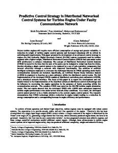
2. Stochastic Characteristics of NCS in Operation Processes A networked process control system with a two-level hierarchical control architecture shown in Figure 1, in which a process plant is controlled by a PID controller at the plant site and the controller can also be self-tuned by a neural network at the remote site, is proposed to improve the performance of the closed-loop system. In this system, the output signal 𝑦(𝑘) of the plant is synchronously measured with ideal sampler 𝑆 at a sampling rate 1/𝑇. The digital controller uses the information of the plant transmitted through the networks to update the new set of the control parameters. The parameter values transmitted through networks and held by a zeroorder holder 𝐻 are then transmitted to drive the plant. 𝑦(𝑘) ∈ 𝑅1 is the input to the controller. 𝑟(𝑘) is the setpoint. NCS operates over a network; data transfers between the controller and the remote system will inevitably introduce network delays; that is, the output quality 𝑦(𝑘) from the current time point 𝑘 is often unavailable before the measurement is sent to the controller at the current time point due to network delays. Likewise, the control input 𝑢(𝑘) from the current time point 𝑘 is also unavailable after the control action is calculated

Mathematical Problems in Engineering

𝑟(𝑘)

+

−

At the plant site PID

3 propagation delay of the network (𝑇𝑝 ). The total time delay can be expressed as [20]

𝑢(𝑘)

𝜏ca

𝐾𝑃 , 𝐾𝐼 , 𝐾𝐷

Process

𝑦(𝑘)

𝜏sc

Network At the remote site Neural network

𝑇delay = 𝑇pre + 𝑇wait + 𝑇post + 𝑇tx + 𝑇𝑝 .

−𝑦(𝑘)

𝑟(𝑘)

Figure 1: Networked process control system.

at the current time point. 𝜏ca denotes the induced delay between the controller and the actuator and 𝜏sc stands for the induced delay between the sensor and the controller. The controlled process is nonlinear no matter whether it is a continuous or batch process. The PID controller control variable 𝑢(𝑘) at the plant site is 𝑢 = 𝑢𝑠 + (𝐾𝑃 𝑒 + 𝐾𝐼 ∫ 𝑒𝑑𝑡 + 𝐾𝐷

𝑑𝑒 ), 𝑑𝑡

(1)

where 𝑢𝑠 is the bias value. 𝑒(𝑘) = 𝑟(𝑘) − 𝑦(𝑘) is the output (𝑦(𝑘)) error deviated from the setpoint. 𝐾𝑃 , 𝐾𝐼 , and 𝐾𝐷 are known as the proportional gain, the integral time constant, and derivative time constant, respectively. In Figure 1, the control structure is similar to an adaptive control structure, but the parameters of the PID controller are adjusted via the backpropagation network control system. The control parameters 𝐾𝑃 , 𝐾𝐼 , and 𝐾𝐷 transmitted through networks and held by a zero-order holder 𝐻 are 𝐾𝑃 (𝑡) = 𝐾𝑃 (𝑘𝑇) 𝐾𝐼 (𝑡) = 𝐾𝐼 (𝑘𝑇) 𝐾𝐷 (𝑡) = 𝐾𝐷 (𝑘𝑇)

for 𝑘𝑇 ≤ 𝑡 < 𝑘𝑇 + 𝑇

(2)

And they are then transmitted to the controller to drive the plant. In networked control systems, a continuous signal is sampled, encoded in digital format, transmitted over the network, and finally decoded at the receiver’s side. The overall delay between sampling and eventual decoding at the receiver can be highly variable because both the network access delays and the transmission delays depend on highly variable network conditions, such as congestion and channel quality [19]. In a networked control system, message transmission delay can be divided into two parts: device delay and network delay. The device delay includes the time delay at the source and the destination nodes. The time delay at the source node includes the preprocessing time, 𝑇pre , and the waiting time, 𝑇wait . The time delay at the destination node is only the postprocessing time, 𝑇post . The network time delay includes the total transmission time of a message, 𝑇tx , and the

(3)

The waiting time 𝑇wait may be significant due to the amount of data sent by the source node, the transmission protocol, and the traffic on the network. 𝑇wait is random in most cases. The postprocessing time 𝑇post is negligible in a networked control system compared with other time delays. The above delays in networked control systems can be obtained by time-stamping techniques although they are normally not available [5]. In the networking area, random network delays have been modeled by using various formulations based on probability and the characteristics of sources and destinations [21]. In most cases, the network-induced time delays are random and are not Gaussian. Packet dropouts result from transmission errors in physical network links, which is far more common in wireless than in wired networks, or from buffer overflows due to congestion. Long transmission delays sometimes result in packet reordering, which essentially amounts to a packet dropout if the receiver discards “outdated” arrivals [22]. The packet loss is another random factor in networked control systems. This means that in general the system output will be very unlikely to be a Gaussian noise, leading to a nonGaussian closed-loop tracking error when the control input is applied to the system. Thus, the randomness measure of the tracking error via the use of variance would not be sufficient in characterizing the performance of the closedloop system. Therefore, the problems considered in this paper can be formulated to design a proper controller such that the shape of the tracking error of NCSs is made as narrow as possible.

3. Design of an NCS Controller The output variable of the controlled processes over the communication system is subjected to the network delay of the uncertain duration and/or stochastic disturbances. It can be treated as a random variable that follows a specific PDF. To adjust the shape of PDF, the entropy is used here. Entropy has a more general meaning to arbitrary random variables than mean or variance. When entropy is minimized, all the moments of the error PDF (not only the second moment) are constrained [22]. Consequently, it can be used to measure and form a design criterion for general dynamic stochastic systems subject to arbitrary random inputs whose PDF can be of any shape. The application of entropy in control and estimation is developed in this section. 3.1. Estimation of Error PDF and Its Entropy. In practical applications, PDF of the tracking error in NCSs is often unknown a priori. A data-driven method that can get the error PDF 𝛾̂𝑒 (𝑧) from the error samples 𝑒𝑘 is employed, where 𝑧 represents the current error, which is a random variable. The error data are obtained by subtracting the process output as actually received by the controller from the setpoint in a given time period. Using the Parzen method [22], the error PDF 𝛾̂𝑒 (𝑧) is approximated as the weighted

4


sum of the 𝐾 Gaussian kernel function defined as 𝜅(𝑧, 𝜎2 ) = (1/√2𝜋𝜎) exp(−(𝑧 − 𝑒(𝑘))2 /2𝜎2 ) with the mean located at the error data point 𝑒(𝑘) as 1 ∑ 𝜅 (𝑧 − 𝑒 (𝑘) , 𝜎2 ) , 𝐾 𝑘=1

𝜏ca

𝐻𝑆 (𝑒) = − ∫

∞

−∞

𝛾𝑒 (𝑧) log 𝛾𝑒 (𝑧) 𝑑𝑧.

𝑒𝑘

(5)

When Shannon entropy definition is used along with this PDF estimation, the calculation of Shannon entropy becomes very complex, whereas the calculation of Rényi quadratic entropy leads to a simpler form. Rényi’s entropy with order 𝑆 of the tracking error is given by ∞ 1 log ∫ 𝛾𝑒𝑆 (𝑒) 𝑑𝑒. 1−𝑆 −∞

(6)

3.2. General Minimum Entropy Based Tuning Neural PID Network. Unlike the conventional deterministic controller design seeking a control input that minimizes the difference between the process output and the desired output at the next time step, the goal of the proposed controller design is to determine control parameters that minimize the shape of error PDF, for the output over NCS is stochastic. The objective is expressed as min 𝐻 = − min log ∫ 𝛾𝑒2 (𝑧) 𝑑𝑧 = − min log 𝑉, 𝐾𝑃 ,𝐾𝐼 ,𝐾𝐷

𝐾𝐼

(4)

where the multidimensional Gaussian function with a radially symmetric variance 𝜎2 is used here for simplicity. For minimizing the range of the error and maximizing the concentration of the error about mean of the error PDF at the same time, the entropy of the error should be minimized. The entropy (𝐻) of the error PDF can be calculated using Shannon entropy

𝐾𝑃 ,𝐾𝐼 ,𝐾𝐷

𝐾𝑃

𝐾

𝛾̂𝑒 (𝑧) =

𝐻 (𝑒) =

𝜏sc

𝐾𝑃 ,𝐾𝐼 ,𝐾𝐷

(7) where the order of Rényi’s entropy is set to be 𝑆 = 2 owing to the computational efficiency. The above objective function is calculated for the present instant time point 𝑘 only. 𝑉𝑘 is information potential (IP) of quadratic Rényi’s entropy at the time point 𝑘. It can be calculated in closed form from the samples using Gaussian kernels as

. ..

𝑟𝑘

1

1

Figure 2: Structure of a neural network in NCS.

to induced random delays. Consequently, in this research, a self-tuning neural PID control scheme is proposed in Figure 2, where a neural network is used to tune the parameters of the conventional PID controller similar to the adjustment made by an experienced operator. Like the human operator who has accumulated past experience and knowledge on the controlled system and knows how to do the adjustment, the neural network can store such information and digest it for the final adjustment because neural networks have the function approximation abilities, learning abilities, and versatilities that can adapt to unknown environments. Thus, the operator’s experience and knowledge can be included into a neural network and the network is trained based on the past data history. Finally, the trained neural network can be used as means to tune the PID controller parameters online. Using a three-layered neural network shown in Figure 2, the learning rule that finds the suitable PID parameters is realized. Thus, in the present neural network values, the setpoint 𝑟(𝑘), the current error 𝑒(𝑘), the induced delay between the controller and the actuator 𝜏ca , and the induced delay between the sensor and the controller 𝜏sc are denoted by 𝑂1(1) , 𝑂2(1) 𝑂3(1) , and 𝑂4(1) . The outputs at the output layer are 𝐾𝑃 , 𝐾𝐼 , and 𝐾𝐷, all of which are denoted by 𝑂1(3) , 𝑂2(3) , and 𝑂3(3) . Then the outputs of a single hidden layer neural network can be computed via the following steps. The input layer is 𝑂0(1) = 1,

𝑂1(1) = 𝑟𝑘 ,

𝑂3(1) = 𝜏ca ,

𝑉𝑘 = ∫ 𝛾𝑒2 (𝑧) 𝑑𝑧 2

1 𝑁 ≅ ∫ ( ∑𝜅 (𝑧 − 𝑒𝑖 , 𝜎2 )) 𝑑𝑧 𝑁 𝑖=1

𝐾𝐷

𝑂2(1) = 𝑒𝑘 ,

𝑂4(1) = 𝜏sc .

(9)

The input and the output of the hidden layer are (8)

1 𝑁 𝑁 ≅ 2 ∑∑ 𝜅 (𝑒𝑖 − 𝑒𝑗 , 2𝜎2 ) . 𝑁 𝑖=1𝑗=1 Although the PID controller is widely utilized because of the simple structure and the intuitive physical meanings, it is difficult to tune proper PID parameters in NCSs owing

4

(2) (1) net(2) 𝑝 (𝑘) = ∑ 𝑤𝑝𝑞 𝑂𝑞 (𝑘) ,

𝑝 = 1, 2, . . . , 𝑃

𝑞=0

𝑂𝑝(2) (𝑘) = 𝑓 (net(2) 𝑝 (𝑘)) , 𝑂0(2) (𝑘) = 1,

𝑝 = 1, 2, . . . , 𝑃

(10)


5

where 𝑃 is the number of hidden neurons. The input and the output of the output layer are 𝑃

(3) (2) net(3) 𝑙 (𝑘) = ∑ 𝑤𝑙𝑝 𝑂𝑝 (𝑘) ,

𝑙 = 1, 2, 3

𝜕𝑦 (𝑘) 𝜕𝑢 (𝑘)

𝑝=0

𝑂𝑙(3) (𝑘) = 𝑔 (net(3) 𝑙 (𝑘)) , 𝐾𝑃 = 𝑂1(3) (𝑘) ,

𝜕𝑦(𝑘)/𝜕𝑢(𝑘) can be replaced by sgn(𝜕𝑦(𝑘)/𝜕𝑢(𝑘)) or it can be calculated by the model prediction algorithm of the plant under the assumption of 𝑢(𝑘 − 𝑖) ≈ 𝑢(𝑘 − 𝑖 + 1) when the proper sampling of the control system is applied as

𝑙 = 1, 2, 3

𝐾𝐼 = 𝑂2(3) (𝑘) ,

𝐾𝐷 = 𝑂3(3) (𝑘) ,

𝑘

= (11)

where 𝑤𝑝𝑞 and 𝑤𝑙𝑝 are weights trained in the neural networks. The initial values of the weight are selected from the uniform distribution across a small range [−1 1]. 𝑓(𝑥) = (𝑒𝑥 − 𝑒−𝑥 )/(𝑒𝑥 + 𝑒−𝑥 ) and 𝑔(𝑥) = 𝑒𝑥 /(𝑒𝑥 + 𝑒−𝑥 ), known as the activation functions, perform the weighted sum of the incoming signals from the input layer and the hidden layer, respectively. With the input layer and the hidden layer, the bias is introduced into the first node. In order to derive the self-tuning algorithm of the PID controller, the cost function defined in (7) should be minimized. Based on the steepest descent approach, at the output layer, we have

𝑘 𝜕𝑢 (𝑘 − 𝜏ca ) 𝜕𝑦 (𝑘) 𝜕𝑢 (𝑘 − 2) ⋅⋅⋅ × ≈ . 𝑘 𝑘) 𝜕𝑢 (𝑘 − 1) 𝜕𝑢 (𝑘 − 𝜏ca + 1) 𝜕𝑢 (𝑘 − 𝜏ca (15)

Also, 𝜕𝑢 (𝑘) 𝜕𝑂𝑙(3) 𝑒 (𝑘) − 𝑒 (𝑘 − 1) { { { = {𝑒 (𝑘) { { {𝑒 (𝑘) − 2𝑒 (𝑘 − 1) + 𝑒 (𝑘 − 2) 𝜕𝑂𝑙(3)

Δ𝑤𝑙𝑝 (𝑘) = 𝑤𝑙𝑝 (𝑘) − 𝑤𝑙𝑝 (𝑘 − 1) = − 𝜂1

𝜕𝑉 𝜕𝐻 (𝑒 (𝑘)) ⇐⇒ 𝜂 𝑘 , 𝜕𝑤𝑙𝑝 𝜕𝑤𝑙𝑝

𝜕𝑦 (𝑘) 𝜕𝑢 (𝑘 − 1) 𝜕𝑦 (𝑘) 𝜕𝑢 (𝑘 − 𝜏ca ) = 𝑘) 𝑘 ) 𝜕𝑢 (𝑘) 𝜕𝑢 (𝑘) 𝜕𝑢 (𝑘 − 𝜏ca 𝜕𝑢 (𝑘 − 𝜏ca

𝜕net(3) 𝑙

(12)

Consider the following: where 𝜂1 or 𝜂 is the learning factor.

𝐾 𝐾 1 = ∑ ∑ (𝑒 (𝑘2 ) − 𝑒 (𝑘1 )) 𝜅 (𝑒 (𝑘1 ) − 𝑒 (𝑘2 ) , 2𝜎2 ) 2 2 2𝐾 𝜎 𝑘 =1𝑘 =1 1

(16)

At the hidden layer, 𝜕𝑉𝑘 𝜕𝑤𝑝𝑞

(17)

𝜕 [𝑉𝑘 ] 𝜕𝑤𝑝𝑞 =

𝐾 𝐾 1 ∑ ∑ (𝑒 (𝑘2 ) − 𝑒 (𝑘1 )) 𝜅 (𝑒 (𝑘1 ) − 𝑒 (𝑘2 ) , 2𝜎2 ) 2 2 2𝐾 𝜎 𝑘 =1𝑘 =1 1

(13)

2

×[

𝜕𝑒 (𝑘) 𝜕𝑤𝑙𝑝 =−

𝑙=3

𝜕net(3) 𝑙 = 𝑂𝑝(2) . 𝜕𝑤𝑙𝑝

2

𝜕𝑒 (𝑘1 ) 𝜕𝑒 (𝑘2 ) − ] ×[ 𝜕𝑤𝑙𝑝 𝜕𝑤𝑙𝑝

𝑙=2

(3) (3) = 𝑔󸀠 (net(3) 𝑙 (𝑘)) = 𝑂𝑙 (1 − 𝑂𝑙 )

Δ𝑤𝑝𝑞 (𝑘) = 𝑤𝑝𝑞 (𝑘) − 𝑤𝑝𝑞 (𝑘 − 1) = 𝜂

𝜕 [𝑉 (𝑒 (𝑘))] 𝜕𝑤𝑙𝑝

𝑙=1

𝜕𝑒 (𝑘1 ) 𝜕𝑒 (𝑘2 ) − ]. 𝜕𝑤𝑝𝑞 𝜕𝑤𝑝𝑞 (18)

(3) (3) 𝜕𝑦 (𝑘) 𝜕𝑦 (𝑘) 𝜕𝑢 (𝑘) 𝜕𝑂𝑙 𝜕net𝑙 =− 𝜕𝑤𝑙𝑝 𝜕𝑢 (𝑘) 𝜕𝑂(3) 𝜕net(3) 𝜕𝑤𝑙𝑝 𝑙

(14)

Using the chain rule, 𝜕𝑒(𝑘1 )/𝜕𝑤𝑝𝑞 and 𝜕𝑒(𝑘2 )/𝜕𝑤𝑝𝑞 can be expressed as

𝑙

𝑘 = 1, 2, . . . , 𝐾, where IP shown above is computed using the measurement errors of the past samples. The Jacobian information

𝜕𝑒 (𝑘) 𝜕𝑤𝑝𝑞 (𝑘) =−

𝜕𝑦 (𝑘) 𝜕𝑢 (𝑘) 𝜕𝑦 (𝑘) =− 𝜕𝑤𝑝𝑞 (𝑘) 𝜕𝑢 (𝑘) 𝜕𝑤𝑝𝑞 (𝑘)

6

Mathematical Problems in Engineering (3) (3) 𝜕𝑦 (𝑘) 𝜕𝑢 (𝑘) 𝜕𝑂𝑙 (𝑘) 𝜕net𝑙 (𝑘) =− ∑ 𝜕𝑢 (𝑘) 𝑙 𝜕𝑂(3) (𝑘) 𝜕net(3) (𝑘) 𝜕𝑂𝑝(2) (𝑘)

×

𝑙

𝑙

𝜕𝑂𝑝(2) (𝑘) 𝜕net(2) 𝑝 (𝑘)

𝜕net(2) 𝑝 (𝑘) 𝜕𝑤𝑝𝑞 (𝑘)

𝑘 = 1, 2, . . . , 𝐾, (19) where 𝜕net(3) 𝑙 (𝑘) 𝜕𝑂𝑝(2)

𝜕𝑂𝑝(2) (𝑘) 𝜕net(2) 𝑝

(𝑘)

(𝑘)

(3) = 𝑤𝑙𝑝

(2) (2) = 𝑓󸀠 (net(2) 𝑝 (𝑘)) = 𝑂𝑝 (1 − 𝑂𝑝 )

𝜕net(2) 𝑝 (𝑘) 𝜕𝑤𝑝𝑞 (𝑘)

(20)

= 𝑂𝑞(1) (𝑘) .

Although IP (8) calculation can be done through the Monte Carlo method, it is preferred to find a more practical solution using sliding windowing. Supposing that the estimate 𝑉𝑘 (𝑒) for the tracking error has been obtained at the 𝑘th run, the recursive estimation algorithm for 𝑉𝑘 (𝑒) of the tracking error can be obtained by using the new sample 𝑒(𝑘 + 1) as follows: 𝑉𝑘+1 (𝑒) ≅ (1 − 𝜆) 𝑉𝑘 (𝑒) +

𝜆 𝑘 ∑ 𝜅 (𝑒 (𝑖) − 𝑒 (𝑘 + 1) , 2𝜎2 ) , 𝐿 𝑖=𝑘−𝐿+1

(21)

where 0 ≤ 𝜆 < 1 is the forgetting factor. 𝐿 is the window length. The size of window 𝐿 should be selected to contain the dynamic characteristics of the plant and network induced delays. Note that even if the sliding windowing is used to produce the information potential, the objective function is still optimized for the present instant 𝑘 only. 3.3. Online Updating PID Controller Based on SPC Monitoring Chart. The conventional control parameter adjustment is triggered on the noise-free or noise-filtered data. However, it has the disadvantage of postponing the parameter adjustment until after an influent transient has subsided. Noise, on the other hand, can induce unjustified control parameter changes, which would, in turn, induce incorrect control action. Process variations in our problem may indeed be a classical electronic type of instrumentation noise and/or packet loss caused by the communications on the employed networks, but they can also be successive, small but real transient in the process output commonly because of external disturbance changes. Thus, in the past, process variations were classified into the common cause and assignable cause variations in manufacturing and service industries. A common cause variation is inherent in the process and is impossible or hard to be eliminated. It is assumed that the sample comes from a known probability distribution.

Based on Shewhart’s classification, Deming (1982) argued the special cause of variations as “something special, not part of the system of common causes” [23] should be identified and removed from the root. If an error value is calculated from noisy measurements, the variable error will be a random distribution variable. Even if controlled processes are well designed and carefully maintained, a certain amount of inherent natural variability is unavoidable. The mechanism that assesses the performance of the control loop for the current operation is the control chart. The chart summarizes the results obtained for the process conducted under the minimum variance. To detect if there is deviation from the minimum bounds in the current operations, a statistical hypothesis testing approach can be applied to the control output error at each time point. If the controlled process is at a steady state, one can conventionally calculate the error distribution function (4). Based on the traditional statistical process control (SPC) method, the upper (𝑈) and the lower (𝐿) control limits for the error are ∫

𝐿

−∞

𝛾̂𝑒 (𝑧) 𝑑𝑧 =

𝛼 , 2

∫

+∞

𝑈

𝛾̂𝑒 (𝑧) 𝑑𝑧 =

𝛼 , 2

(22)

where 𝛼 represents a probability of falsely rejecting the hypothesis when, in fact, it should be accepted. The selected area 𝛼 under the normal operation is quite small. In this study, 𝛼 is 0.05. 𝐿 and 𝑈 limits of the integral indicate that the desired value of the probability density function will be 𝑈 between 𝐿 and 𝑈 with the integral value (∫𝐿 𝛾̂𝑒 (𝑧)𝑑𝑧) is equal to 1 − 𝛼 (22). Thus, whenever the process is around the setpoint, it is highly unlikely that the discrepancy between the observed and the setpoint values will be out of the lower and the upper limits. One aspect of the SPC philosophy is to accept the normal process variability without reporting any change in value unless the cause is identified [24, 25]. Equation (22) is numerically tractable using the probability model to calculate the thresholds (𝐿 and 𝑈) and detect any departure of the process from its standard behavior. Applying the above control limits to the measured error variable, one would retain the PID controller parameters in the local plant until there is statistically sufficient evidence that the error value is changed. This means that an SPC control chart is superimposed to monitor when the controlled system departures from the target so that the value of the NN-PID controller parameters can be regulated. Therefore, the proposed two-level hierarchical control architecture can be summarized by the following steps. Step 1. Calculate the tracking error in NCSs {𝑒(𝑘1 ), 𝑒(𝑘2 ), . . . , 𝑒(𝑘𝑁)} and IP based on the sliding windowing using (21). Step 2. Train neural networks offline based on the historical data and the conventional turning method, like ITAE (integral of the time-weighted absolute error). Of course, the historical data should cover the desired operation region. A good initial model can be achieved. Also, use (21) to construct 𝐿 and 𝑈 control limits. Then the weights of the neural networks are updated by (12) and (17).


7

Step 3. Check whether the controlled variable is “in statistical control” or not. If the process that is operating with only chance causes of variation present is “in statistical control,” keep the same controller parameters; otherwise, update 𝐾𝑃 , 𝐾𝐼 , and 𝐾𝐷 obtained via neural networks.

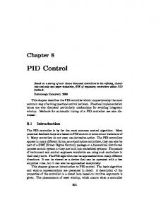
Neural network

At the remote site Internet

Step 4. Formulate the control input 𝑢(𝑘) by (1) and apply the control input 𝑢(𝑘) to actuate the plant, set 𝑘 ← 𝑘 + 1, and repeat Step 1. At the local site PC

Note 1. Neural network adjusts the parameters of the controller in terms of the tracking error. The changes of the tracking error cannot be obtained soon when the operating point changes or the disturbance occurs. Nevertheless, the changes of the tracking error can be obtained eventually after a period of transmitting time due to the closed-loop feedback. Note 2. The kernel size (the window width of the Parzen estimator) can be set experimentally after a preliminary analysis of the dynamic range of the tracking error. Some clustering analysis techniques can be applied to get the proper kernel size. To ensure that the proposed algorithm can track the desired output of the controlled system, the convergence condition for the proposed algorithm should be satisfied and is derived as follows. Theorem 1. If the learning factor satisfies 0 < 𝜂 < 1/max𝑖 |𝜆 𝑖 |, the weights of the neural networks are convergent in mean square sense. The weights of the neural networks can be rearranged in a line and denoted as a vector 𝑊. Equations (12) and (17) can be summarized as follows: 𝑊 (𝑘 + 1) = 𝑊 (𝑘) + 𝜂∇𝑉 (𝑊 (𝑘)) ,

(23)

where ∇𝑉(𝑊(𝑘)) is the gradient of 𝑉𝑘 given in (13) or (18) evaluated at 𝑊(𝑘). Perform the Taylor series expansion of the gradient ∇𝑉(𝑊(𝑘)) around the optimal weight vector 𝑊∗ as 𝜕∇𝑉 (𝑊∗ ) ∇𝑉 (𝑊 (𝑘)) = ∇𝑉 (𝑊 ) + (𝑊 − 𝑊∗ ) . 𝜕𝑊 ∗

(24)

∗

Define a new weight vector space 𝑊 = 𝑊 − 𝑊 and yield 𝑊 (𝑘 + 1) = [𝐼 + 𝜂𝑅] 𝑊 (𝑘) ,

(25)

where the Hessian matrix 𝑅 = 𝜕∇𝑉(𝑊∗ )/2𝜕𝑊 = 𝜕2 𝑉(𝑊∗ )/ 𝑇 2𝜕𝑊2 . Let Ω = 𝑄 𝑊, and 𝑄 is the orthonormal matrix consisting of the eigenvalues of 𝑅. Thus, Ω (𝑘 + 1) = [𝐼 + 𝜂Λ] Ω (𝑘) ,

(26)

where Λ is the diagonal eigenvalue matrix with entries ordered in correspondence with the ordering in 𝑄. It yields Ω𝑖 (𝑘 + 1) = [1 + 𝜂𝜆 𝑖 ] Ω𝑖 (𝑘) , 𝑖 = 1, 2, . . . , 𝑃 (𝑄 + 1) + 3 (𝑃 + 1) .

(27)

PT Air

Figure 3: Schematic diagram of the air-pressure tank control loop over the network.

Define ΔΩ𝑖 (𝑘) = Ω𝑖 (𝑘 + 1) − Ω𝑖 (𝑘). Since the eigenvalues of the Hessian matrix 𝑅 are negative, |1 + 𝜂𝜆 𝑖 | < 1 can guarantee that the 𝑖th weight of the neural networks obtains a stable dynamics in mean square sense. Therefore, the following inequality can ensure that the proposed algorithm is convergent in mean square sense: 0