Stone (1960) and Laming (1968) proposed early versions of sequential sampling ... chis paper. Address for correspondence: Andrew Hearhcotc. Depamenc of ...
I57
Neuromorphic Models of Response Time Andrew Heathcote The University of Newcastle A new approach to modelling response time is proposed, based on the activation dynamics of simplified
neural units.The proposed neuromorphic decision units are dissipative and have bounded activation, as do real neurons. A decision is made either when the unit's activation exceeds a threshold or when it converges, using a criterion based on the derivative of activation. First, the relationship between varieties of neuromorphic and sequential sampling models is reviewed. Mathematical and simulation results are presented both for deterministic and random versions of the neuromorphic units. These results are used to highlight strengths and weaknessesof this new approach to dynamic models of decision making.
T
he models developed here were inspired by the similarity between sequential sampling models of choice and response time and first order approximations to neural dynamics, such as those used by Carpenter and Grossberg (1987) and Kohonen (1993). The term ncuromophic reflects the fact that the models are based on the (simplified) structure of biological nervous systems. The next section reviews sequential sampling models and a number of theoretical and empirical issues that have driven their development. The following section motivates the structure of the neuromorphic models with reference to empirical issues and constraints from physical instantiation. The next two sections develop the mathematical detail of the models, and the final section discusses their strengths and weaknesses. SEQUENTIAL SAMPLING MODELS
The following brief review can not do justice to the scope of sequential sampling models (see Busemeyer & Townsend, 1993; Laming, 1968; Link, 1992; Link & Heath, 1975; Ratcliff, 1978; Smith. 1995). Instead, the review is selective, with the aim of illustrating the many similarities of neuromorphic and sequential sampling models. In some cases, versions of the neuromorphic models are special cases of the sequential sampling models, and in other situations they are more general. Sequential sampling is the dominant dynamic model of decision making (see Luce, 1986 for a review). Dynamic decision models predict not only which choice is made, but also response time (RT). A decision is made when the sum of a series of samples from a signal exceeds a criterion. Use of the sum promotes accurate decisions by averaging over sample-tosample noise in the signal. As more samples are taken, noise is suppressed but RT is increased. Hence, a trade-off between speed and accuracy (Luce, 1986, Section 6.5) is a fundamental prediction of sequential sampling models. When the signal-tonoise ratio is small, slow responding promotes accuracy. Under time pressure, fast decisions can be made, but the decision will be inaccurate unless the signal-to-noise ratio is large. Noise, in the form of random sample-to-sample fluctuation in the signal, may be introduced from a number of sources. Link (1992) suggests that sample-to-sample noise is due to Poisson fluctuation in the transmission of signals in the nervous system. At a coarser temporal scale, Busemeyer and Townsend (1993) suggest that subjects switch attention between different consequences of the choice on each sample.
Decisions based on a sum of samples allow the subject to weigh a large range of alternatives without having to hold them in short-term memory simultaneously. Stone (1960) and Laming (1968) proposed early versions of sequential sampling models. Subjects sample a signal with mean M at regular time intervals of length dr. Hence, each sample has mean size M and is added in exactly dt time units. A response is made when the sum of samples exceeds a criterion, C. In the following I will use the term acrivarion to refer to the sum of samples. RT equals the time per sample multiplied by the number of steps taken until the sum first equals or exceeds C. The model is often called a rundom walk because the sum follows a jagged path reminiscent of a particle undergoing Brownian motion. The random walk is a discrete process. As the time unit, dr, goes to zero it becomes equivalent to a continuous Wiener diffusion process. Summation becomes integration with infinitesimal mean step size or drift, M, and infinitesimal variance or diffusion rate, 0'. The diffusion process, with normally distributed sample-to-sample noise, was first proposed as a model of simple RT by Emerson (1970). When drift is normally distributed and C >> M. mean X dt for the discrete case), and overall RT has an RT = inverse Gaussian distribution. This single criterion case can model simple RT, where the subject responds contingent only on the detection of a change in the stimulus. Multiple criteria or barriers model more complex choice tasks.In the two choice case, for example, an adaptation level can be subtracted from the signal so that samples from one class of stimuli have negative mean drift and the other class has positive mean drift (Link & Heath, 1975). The choice made depends on which barrier is crossed first. The RT distribution for the two-alternative Wiener diffusion model is given in Ratcliff (1978). It is more complex than the distribution for the single barrier model because the RT distributions for each choice can be a mixture of correct and incorrect responses.
(5
Varieties of Sequential Sampling Models
In Link and Heath's (1975) relative judgement theory, a random walk is driven by the difference between the signal and an adaptation level or referent. Subjects can control the distance between response barriers, the starting position of the random walk, and magnitude of the referent. This theory not only predicts RT. but is also able to account for variations of
Thanks (0 Richard Heath. Doug Mewhom Mike Humphreys, and Jerr, Burerneyer. Scott Brown. and Stcphan Levendowsky for comment on drafts of chis paper. Address for correspondence: Andrew Hearhcotc. Depamenc of Psycholog. The Univeniv of Nmurd+ N-dc NSW 2308. A u d i E-mail: h ~ ~ c o c ~ p ~ c h o l o M . n a w c u r l L c d u l u A u d i a n journal of Psycholoa Vol. 50. No. 3. I998 pp. 1.57-1 64
I58
Andrew Huchcote
response probability modelled by static theories such as signal detection theory (SDT) and finite state theories (see Green & Swets, 1966). Link and Heath (1975) demonstrated that their model can produce similar receiver operating characteristics (ROCs) to SDT by changing the random walk’s starting point. Differences in the magnitude of mean drift rates (and/or their varjances) from the two stimulus classes result in asymmetric ROC curves, assumed to be due to unequal variance in SDT. Increasing either the distance between the barriers or the magnitude of the drift rate causes increasingly curved ROCs associated with an increase in sensitivity in SDT. A more recent version of this model, wave theory, proposed by Link (1992), is consistent with an impressive list of psychophysical phenomena, including the psychometric function; the interval of uncertainty; Fechner’s. Weber’s, and Steven’s Laws; as well as ROC results. Despite the success of both wave theory and models based on the Wiener diffusion process, without elaboration both are unable to model an important finding related to speed-accuracy trade-off, the conditional mean RT effect (Heath, 1992). Under speed instructions, mean error RT tends to be faster than mean correct RT. whereas, under accuracy instructions, errors tend to be slower than correct responses. Link and Heath (1 975) showed that, when the moment-generating function of a random walk’s step size is symmetric, correct and error mean RTs at the same barrier are equivalent. As the Poisson moment-generating function is symmetric (as are the moment-generating functions of most commonly used noise distributions), wave theory cannot account for the conditional mean RT effect. The Wiener diffusion model for two choices also predicts equal error and correct mean RT. Two accounts of the conditional mean RT effect have been proposed. One account adds variability between trials to model parameters, the starting point and drift rate. Laming (1968) suggested that the starting point of a random walk might vary from trial to trial under speed instructions due to sampling before the onset of the stimulus. Fast and inaccurate responses will occur when the starting point is near the barrier for the wrong choice. In contrast, slow errors are produced when between-trial variability is introduced to the drift rate of a two-alternative Wiener diffusion model (Ratcliff, 1978). If accuracy stress causes an increase in the intertrial variability of drift rates, slow errors for accurate responding can be explained. Ratcliff (1988) notes that fast errors can also be obtained with drift distributions that have heavier tails than the normal distribution, although he did not pursue this approach. The second account introduces systematic changes in the signal strength over the course of a trial. Heath’s (1981) tandem random walk model, and his later generalisation for temporally and spatially nonstationary inputs (Heath, 1992). can account for both aspects of the conditional mean RT effect. If a response is initiated when the input is increasing, mean error RT is faster than mean correct RT. If the response is made when the input is stationary, correct and error mean RTs are equal. If a response is made when the input is decaying, mean error RT is slower than mean correct RT. Heath (1992) and Smith (1995) discussed the physiologically interesting case where a nonstationary input is the result of a deterministic cascade process. Another variety of sequential sampling model assumes that the process of sample integration, rather than the signal. changes over the course of a trial. For example, some signal strength might be lost in the summation or integration process. Unlike a random walk or diffusion, a “leaky integator” is dissipative: it loses some of the signal strength in the process of integration. Smith (1995) and Busemeyer and Townsend
(1993) describe sequential sampling models in which the leakage is dependent on the activation of the unit. Consequently, the effective drift from a constant input signal decreases to zero as activation grows, and so activation achieves equilibrium. Busemeyer and Townsend (1993) modulate state-dependent leakage rates to model the finding that, in both animal and human decision making, avoidanceavoidance decisions take longer than approach-approach decisions. Their Decision Field Theory modulates state-dependent leakage rates to model the finding that, in both animal and human decision making, avoidance-avoidance decisions take longer than approach-approach decisions. Decision field theory also accounts for a range of phenomena in risky decision making and matching. Activation-dependent leakage can answer Heath’s (1962) “finite RT dilemma”: why can subjects not become arbitrarily accurate by sampling for a sufficient time? Accuracy for a lossless random walk model increases indefinitely as more samples are taken. Hence, increased accuracy can always be obtained by placing the decision barriers further away from the starting point. For a state-dependent leaky integration model, in contrast, activation tends to an asymptote, so a decision criterion cannot be placed arbitrarily far from the asymptote. Mechanisms do exist within lossless random walk models that can address the finite RT dilemma, for example, Ratcliff s (1978) addition of trial-to-trial as well as sample-to-sample noise. While continued sampling can arbitrarily reduce sample-to-sample noise, it can do nothing to reduce trial-totrial noise. When sufficient samples have been taken to reduce sample-to-sample noise below trial-to-trial noise, continued sampling has little effect on the overall accuracy of the decision. Ratcliff and Van Zandt (1995) discuss the roles of both sample-to-sample and trial-to-trial noise in a diffusion model of a signal detection task. As Luce (1986) notes, “the original wrinkle introduced [by Ratcliff (1978) which] ... has given the [diffusion] model a great deal of flexibility, is that rates are in fact random variables over otherwise identical trials. ... l h s added freedom is adequate to permit the model to mimic a great deal of somewhat surprising data” (p. 439). Clearly, experimental data may contain both sample-tosample and trial-to-trial noise. Sequential sampling models have tended to emphasise sample-to-sample noise, perhaps because of its role in explaining speed-accuracy trade-off. In the next section we will explore why, in neuromorphic models, sample-to-sample noise is not necessary for this purpose. MOTIVATING NEUROMORPHIC MODELS OF CHOICE
The first order behaviour of a neuron is similar to a random walk process in that a neuron integrates inputs over time. However, neurons are dissipative structures, so their integration is leaky. In contrast to a random walk, where a constant input causes activation to increase indefinitely, activation in a neuron converges to a value that is a (usually monotonic) function of a constant input. When input is removed, the neuron returns to baseline firing. Both behaviours are characteristic of a unit with activation-dependent leakage. Secondly, the activation of a neuron is bounded; the unit’s activation cannot be driven above a maximum value no matter how large the input because its sensitivity decreases as activation approaches the bound. In the following section, we will discuss the implications of introducing these constraints to sequential sampling models of response time. Statdependent Leakage
One important reason for inuoducing leakage into neuromorphic models is physical plausibility: state-dependent leaky
-
A u d i J o u d of P~~cholou D M m b r 1998
Neuromorphic Models of Response Time
integration can attain only finite activation for finite inputs, whereas the activation of a lossless integrator diverges to infinity for a constant finite input. With leakage, activation also takes some time to fully reflect the input, a phenomenon commonly measured by a time constant in neural systems. Hence, an activation-dependent leaky integrator has bounded sensitivity, both in time and activation. Speed-accuracy trade-off can be explained by the finite temporal sensitivity of activation-dependent leaky integrators. A fast response is effectively based on a weak signal if it is made before activation has reached equilibrium. Consequently, sample-to-sample noise i s not necessary t o explain speed-accuracy trade-off. While a complete lack of sample-tosample noise is unlikely, it is an interesting question in many experimental paradigms whether performance is dominated by sample-to-sample or trial-to-trial noise. In a recognition memory experiment, for example, variations in study-test lag, and word stimuli, may cause considerable extrinsic noise in inputs over trials within an experimental condition. The neuromorphic models developed here assume that trial-to-trial noise dominates. This was done mostly in the interest of mathematical tractability. Having gained some results with the assump tion of trial-to-trial noise alone, we will return to the issue of sample-to-sample noise in the final section. Leakage also results in decay of activation back to baseline when the input ceases. This is functionally useful for an autonomous decision system because decision units automatically reset between decisions. In contrast, a random walk requires reset by an external controller. Partial return to baseline between closely spaced trials may account for some patterns of sequential dependency in both accuracy and RT, although learning effects in adaptation levels and strategic probability matching are also likely to be important (e.g., Link. 1992, pp. 276293). Representation
Activation-dependent leakage is useful because the decision unit’s asymptotic activation provides an estimate of the magnitude of the input. Hence, the unit’s activation can be used to represent stimulus characteristics as well as to make decisions. In a lossless model, the unit’s activation c o n d n s no information about the magnitude of the input, unless integration time is also known.In an activation-dependent dissipative model, in contrast, activation is a function of the input magnitude independent of integration time (once the unit has converged). Convergent activation provides a point of contact between dynamic and static models of choice. Due to the static nature of SDT, RT predictions do not emerge naturally, although additional mechanisms, such as RT proportional to the difference between signal and criterion, have been suggested (Murdwk & Dufty, 1972). A state-dependent leaky integrator model, in contrast, predicts both RT and accuracy. The static decision variable in SDT is identified with the static activation value of the neuromorphic unit after convergence. Choice can be modelled in the manner of SDT, by comparing the converged activation value to a criterion. RT predictions follow naturally from the time to detect convergence. Response Criteria
The preceding discussion suggests a more radical departure from previous sequential sampling models: using detection of convergence as the criterion for response. Gregson (1992) suggests that a check on the stationarity of the Jabcobian for a system of units can be used in this way. For a single unit. a simple way to detect convergence is to place a criterion on the derivative of activation with respect to time. In the discrete case, the criterion is placed on the size of each sample. A Crite-
I 59
rion on the derivative is convenient for the neuromorphic models described below as they are defined by first order differential equations. The derivative is not so convenient when the neuromorphic model contains sample-to-sample noise, as activation, while being almost everywhere continuous, is almost nowhere differentiable. In the following development, both activation and derivative criteria will be investigated. The two criteria are not incompatible. For example, an activation criterion may be used when a fast response is required and a derivative criterion when an accurate magnitude estimate is required. Both criteria can be problematic for units with activation-dependent leakage. If the input is small, a derivative criterion may be satisfied immediately, whereas an activation criterion may never be Satisfied. Hence, there may be situations when both criteria are applied simultaneously. Activation Bounds
Many neural network models bound a unit’s output activation with sigmoid transformation. The presence of bounds can be motivated by physical realisation: like any physical system, the unit can only take on states within a finite range. The particular choice of bounding function, a smooth sigmoid. is an idealisation for individual neurons, which often exhibit sensitivity thresholds. However, the sensitivity of a collection of neurons, where thresholds vary randomly between neurons, is described by a smooth sigmoid function. For the decision units discussed so far, activation was unbounded. State-dependent leakage ensures that activation does not diverge with integration time, but the dynamic range of the unit remains unlimited. Bounds of some type seem called for on a priori grounds, but, as will be shown in the following development. they also impart functionally useful properties to the neuromorphic units. A second motivation for sigmoid bounds on activation comes from the suggestion that neuromorphic units can represent the input. Back-propagation neural networks use sigrnoid hidden units as they provide universal function approximation abilities (Hornik, Stinchcombe, & White, 1989). One way, therefore, to provide general representational ability is to make asymptotic activation a sigmoid function of input magnitude. Summay
The preceding sections suggest that a neuromorphic model should have both activation-dependent leakage and bounded activation. They also suggest that asymptotic activation be used to represent the magnitude of the input, so neuromorphic units have the dual role of representation and decision. In order to make the representation general, sigmoid bounds are useful. In order to make the representation independent of integration time, a response criterion based on the derivative of activation was suggested, although an activation criterion may also be used in some situations. Finally, emphasis was placed on trialto-trial noise in the model’s parameters. While the likely Occurrence of sample-to-sample noise was acknowledged, it was argued that it could be dominated by trial-to-trial noise, so that models with trial-to-trail noise alone are interesting. at least as a limiting case. DETERMINISTIC MODELS In this section we will examine the deterministic behaviour of
models with a minimal s h c t u r e motivated by the considerations in the previous section. In the next section, we will examine the behaviour of these models with trial-to-trial noise in their inputs. We will consider two types of neuromorphic units based on deterministic models of first order neural dynamics used by Carpenter and Grossberg (1987) and Kohonen (1993).
A u ~ l iJounul i of Psyddow
- December I998
I 60
Andrew Heathcote
Kohoncn Units
Kohonen (1993) suggested that important aspects of dissipative neural dynamics are captured by the differential equation: (1)
i=I-
where x is activation, X its derivative, I is an input, and * x ) a loss function describing activationdependent leakage. For example, consider the simple case where the loss function is linear: y(x) = /3 + ax.By definition, the system described by Equation 1 converges when x = 0. By solving this equation with the latter condition we find that asymptotic or equilibrium activation equals
(I = B) a Hence, the final state of the unit is a linear transformation of the input. A solution for activation, x , at all times, t, is derived by solving Equation 1.
The activation of the unit at = 0 is x ( 0 ) . Unless otherwise stated, we will assume in the following that ~ ( 0= ) 0. Figure la illustrates the solution, with activation converging at an exponentially decreasing rate toward its asymptotic value. Interestingly, the activation update function used by most PDP models, x, = Zw,,xj can be viewed as the equilibrium solution to Equation 1 with I = Z w i j x i , and y ( x ) = x . Similarly, Cohen. Dunbar, and McClelland's (1990) cascade update equation, used to predict RT in the Stroop paradigm, x,,, = ( I - r)x, + T ~ w ; ? , is an Euler's approximation to the same equation with a time constant 7:
neuromorphic model, in contrast, the dynamics of the neural unit alone determine RT. RT predictions for the linear leakage Kohonen unit can be derived by determining the time, f , at which x = a (Equation 3). the activation criterion, and at which x = d (Equation 4). the derivative criterion.
x@)
f
1
= -In( a
I - /3 - u ( 0 ) 1 ) = --In( d a
X(")
-a
-No))
x(m)
-d
(3)
(4)
The second form of both equations specifies the solution'in terms of the asymptotic value of activation
Nm) = -.(I- B) a
For both types of criteria, t decreases as the criteria become less strict. Signal intensity. however, has opposite effects on t, with more intense signals decreasing r for the activation criterion but increasing t for the derivative criteria. Empirical RTs from simple and choice paradigms are usually a decreasing function of signal intensity and an increasing function of response caution. Lf we identify signal intensity with 1 - /3 and response caution with or it is clear that the derivative criterion model is in error for signal intensity predictions: response time is predicted to be an increasing rather than decreasing function of signal intensity. In order to restrict activation within a given range for all input values. the loss function must be nonlinear. Kohonen (1993) bounds activation in the range [-1.11 using:
i,
7
In Cohen and colleagues' model, RT predictions were derived using a combination of.the cascade update rule and a random walk decision unit attached to the output of the network. For a
At equilibrium:
x(m) I
"
o.t/
,f
I l-eT = ___ ranh(-) -I 1 + eT
1.01
C
Similarly, )(x) = c In
L)
-
(1
produces [0, I ] bounded asymptotic activation following a logistic function. Unfortunately, we cannot obtain an explicit expression for t for Kohonen's sigmoid equations as they are not soluble in closed form.' Instead, we proceed by considering a second mechanism for bounding activation, shunting SO
inputs.
100 150 200 ic)
Figure I (a) The g r o h in advation ( x ) as a function of time (t) for Equation I with linear leakage. a = 0.1,j3 = 0.x(0) = 0.and a range of, inputs (I). Note the convergence to asymptotic values ;( = I, 0.5, and 0. I). (b) Asymptotic a d t i o n as a function of input intensity for a shunting sigmoid (thick line a = 0. I , A = 0 = 1) and & ~ n hsigmoids, c = 0.08,0.2. and 0.333 (from steeper to flatter curves respectivety). (c) Activation growth over time with positive inputs, 1. for Equation 7. a = O.OI.A = B = I , r = 0 . (d) t (plotted as dre ordinate) from Equation I0 as a function of /+ (the abcissa), a = 0.I, x(0) = 0,A = B = I , and r = 0.for five values of d. M
i
Groubcrg.Units
Grossberg and co-workers (e.g., Carpenter & Grossberg, 1987) often approximate neural dynamics with the differential equation:
+ f (A - X) - T ( B f X) = ( A F - BT)- xfa + I- + F) (6) Inputs are separated into excitatory ( r )and inhibitory (0
i =
- ( 1 ~
components as is commonly observed in neural systems (note that all parameters and inputs in Equation 6 are positive). The form of Equation 6 given on the right can be usefully
- O ~ m b e I998 r
J o u dof hydlolog).
Neuromorphk Models of Response Time
contrasted with Equation 1. The main difference is that the leakage tenn is a function of the inputs as well as the level of activation. This dependence is called a shunting interaction. The form of Equation 6 on the left makes it clear why activation is bounded in the range [-B, A]. The effect of excitation is scaled by the difference between the present level of activation and A. and the effect of inhibition is scaled by the difference between the present level of activation and -B. Even when an external perturbation leads to x > A or x c -B, the system will be attracted back within the bounds. The equilibrium solution to Equation 6 also shows that activation is bounded in the range [-B.A]:
(7) To compare Equation 7 with Kohonen's tanh sigmoids, where I can be positive and negative, Figure Ib illustrates the case where I+ = I, t = 0 for I 2 0. and t = -I, I+= 0 for I < 0, that is,
The slope of the shunting sigmoid is controlled by the rate constant a. For companion, three tanh sigmoids are also shown. Note that the shunting sigmoid (thick line) tends to have a shorter linear range and is steeper around the origin than the tanh sigmoids, which cover approximately the Same dynamic range. Figure l c illustrates the convergence behaviour of Equation 7. Unlike the linear loss form of Equation 1 (see Figure la), time to convergence (approximately where the graphs become flat in Figure l a and Ic), and hence RT under a derivative criterion, is inversely proportional to input intensity. To obtain an explicit expression for activation as a function of time, we begin by solving Equation 6:
I6I
The effect of increasing signal intensity on t , given the derivative criterion, depends on a balance between a hyperbolically decreasing tendency caused by the scaling factor and logarithmic increase identical to the linear model. Figure Id illustrates the trade-off, plotting t as a function of the derivative criterion, d. and input intensity, r(with f = 0). Note that Equation 10 is valid only when d C [x(m) - do)] as the difference between x at 0 and m is the maximum rate of change of activation. Hence, the negative solutions in the figure are not valid. For larger input values, t is a negatively accelerated, decreasing function of r, consistent with empirical evidence of a decrease in R T with increasing signal intensity. For smalle? values of r, however, t increases with signal intensity. The increasing region reflects approximately linear sensitivity and associated behaviour approximated by Equatib 4. The influence of the increasing region depends on the value of d. Considering Equation 10 with parameters specified as in Figure Id. for example, 1.d = 0.01 (lax criterion, middle curve in Figure Id): t at the point of inflection is 11.57, activation at response is 0.41, and activation at asymptote is 0.46, 2. d = O.OOO1 (strict criterion. upper curve in Figure Id): t at the point of inflection is 44.2, activation at response is 0.1835, and activation at asymptote is 0.184. For the strict criterion, the increasing region occurs for I c 0.023 and in less than 20% of the domain of x ([OJ] for the parameters chosen). With the lax criterion, the increasing region occurs for I c 0.09 and covers almost 50% of the domain of x. The difference between activation at response (i = 6) and asymptote (i = 0) also changes with the criterion. For the strict criterion, the difference is only 0.3%. compared to almost 1 1% for the lax criterion. Overall, the similarity between asymptotic sensitivities shown in Figure 1b suggests that Kohonen's and Grossberg's models will act in a similar manner. We will now turn our attention to the behaviour of the model when the inputs have a stochastic component. It turns out that, in this context, we can make some progress with Kohonen's bounded model as well as with Grossberg's shunting model.
As with the linear version of Kohonen's equation, activation
RANDOM MODELS
converges at an exponentially decreasing rate toward its asymptotic value. Solving for x = a, the activation criterion, and i = d, the derivative criterion:
We will now explore the effect of trial-to-trial noise on the inputs to neuromorphic units. The distribution of the input, I, is assumed to be Gaussian, a plausible assumption in a neural network context as I is the sum of a large number of weighted inputs. We will characterise the model by determining the density function and hazard function for response time. RT density is usually uni-modal and positively skewed, and increases in the mean are usually accompanied by increases in variance and skew (e.g., numerous examples in Luce, 1986, although distributions for very fast responses can be relatively symmetric; see, e.g., Luce, 1986, p. 117 for simple RT to intense auditory stimuli). Examination of density functions will determine if the neuromorphic models share any of these characteristics. The hazard function is defined as probability density divided by the one minus cumulative density, and denotes the chance of an event occumng at time t given it has not already occurred. Luce (1986) suggests that hazard functions can help to differentiate models with similar density functions. For simple RT, ,empirical hazard functions rise to a peak and then descend, especially for intense stimuli. The neuromorphic model hazard functions will be comparrd to this pattern. We will begin by obtaining analytic results for the lossless integrator with an activation criterion. Only the distribution of I is of interest, as x is, by definition, a constant equal to the
(9)
Equations 9 and 10 are similar to the solutions for the linear activation-dependent leakage model (Equations 3 and 4). This occurs because they are both solutions to the general equation: x ( r ) = x ( m ) - [x(w) - X ( O ) ] ~ - ~where , K determines the rate of leakage. As in the linear model, a stricter activation or derivative criterion causes a decrease in t. The models differ in that the scaling factor in the linear model (i)becomes dependent on the inputs 1
( a + r+r)' due to the shunting interaction. For the activatiop criterion, the shunting interaction further enhances the decrease in t with increases in signal intensity.
- December 1998
A u d i a n Journalof Psycholog).
I62
Andrew Hathcocc
criterion. Analytic results were also obtained for asymptotic activation in the Kohonen and Grossberg models. However, the distribution of t for these models must be investigated by Monte Car10 techniques.
For a Kohonen unit with tanh leakage, and given that the density of I , f l l ) , is nomal with mean p and standard deviation a,the density of x, g(x), is:
Lossless Integrator: Analytic Rcsuhr fort
Before examining the dissipative models, we will explore the lossless integrator with normally distributed input, I, and a one-barrier activation criterion, B. For this model, t = BlI is inversely proportional to input intensity and proportional to response caution ( B ) . Distribution functions with only trial-totrial noise are easily obtained because the relationship between barrier crossing time. 1, and the random variable, I , is monotonic and has a differentiable inverse (see DeGroot. 1986, pp. 152-154). Given that the density of 1,flI). is nomal with mean p and standard deviation a,the density of r. g(t), is:
Figure 2 illustrates the effect of varying p and u relative to a reference distribution with p = 10, u = 3 ( B = 3.000 in all cases). Note that the reference distribution is the curve with the second highest peak in all panels of Figure 2. A decrease in p causes an increase in the mode. mean, variance, and skewness and a decrease in the order and peakedness of the hazard function. An increase in CT causes a decrease in the mode, and increase in mean variance and skewness. The hazard function spreads at the same location with increases in a,as does the density function. Kohonen and Grossbeg Units: Analytic Activation Distributions
Closed fonn results for the distribution of asymptotic activation in both Kohonen and Grossberg units can be obtained because the runh. logistic, and shunting sigmoid functions are monotonic and have a differentiable inverse. For Kohonen units with a derivative (i = d) criterion, the activation distribution function is the same as for the asymptotic case, with the exception that the mean, p, is reduced by d. Hence, we will develop results only for the asymptotic case for Kohonen units. 0.007 0.006 0.005
0.001 0.003 0.002
0.001
zoo
400
500
80*?
LOO
1'100
400
600
900 1000
I
(b)
0.005 0.0025 ZOO
400
6W
800
Figure 3 illustrates the properties of g(x) as a function of the mean and standard deviation of the input for c = 1. When p = 0 and u is small. the distribution is approximately normal. but as u increases the distribution flattens and eventually becomes U-shaped as probability mass from the tails builds up at either bound (see Figure 3a). When p is nonzero, the activation distribution becomes skewed, with the degree of skew strorrgly dependent on u (see Figures 3b and 3c). A similar result holds for the logistic bound, as the logistic function is a linear transformation of the rmh function. The effect on of varying d can be seen in Figure 3c, because a stricter convergence criterion is equivalent to increased mean signal strength. If accuracy equals the proportion of the activation distribution passing a criterion in x (e.g., below the origin in Figure 3c). then accuracy is inversely proportional to d. The separation of excitatory (positive) and inhibitory (negative) inputs in Grossberg's shunting equation makes it difficult to determine the distribution of activation across the entire range [-B,A]. We will instead consider the case where there is negligible probability of 1 5 0, and solve for the derivative criterion, .i = d. Note that variation in the criterion, d, for a Grossberg unit is not equivalent to variation in the mean signal strength as it was for a Kohonen unit, due to the shunting interaction. Hence, we must derive an expression for the distribution of activation which includes d. Given that the density of the input signal I, AI). is normal with mean p and standard deviation u,the density of x , g(x), is: I
g(x) =
(w)?
=
d o + *l-(*+cfl
+ d- x ) z e 3( d**a(l Q
I-r
)?
(13)
Figure 4 illustrates that the behaviour of asymptotic Grossberg unit activation is similar to that of asymptotic Kohonen unit activation shown in Figure 3, and that p and d act similarly (note that d is varied over a smaller range than p). Once again, if accuracy equals the proportion of the activation distribution passing a criterion in x (e.g., above x = 0.5 in Figure 4b), then accuracy is inversely proportional to d. In summary, we have found closed form solutions for activation at a derivative criterion, d , for both Kohonen and Grossberg units. We have also shown that variation in d can be used to model speed-accuracy trade-off as a decrease in d produces more accurate responding. The deterministic results for time to satisfy the derivative criterion indicate that the increase in accuracy will be accompanied by a decrease in RT, as found empirically.
1000
1
(C I
Fiaure 2 (a.-b) Probability density functions and (c. d) Hazard functions [with SUPPOK on t = 2W700, except t = 150-700 for p = 10. u = 5 in (d)] for normal input t o a deterministic single barrier random walk 6 = 3000. ( h c) u = 3, p = 12, 10.8 and (b, d) p = 10. u = 2. 3, 5 (iterating over curves from upper to lower).
Figure 3 Asymptotic acrivation distributions for a Kohonen unit with c = I.x = tanh[N(p.cd)] and u = 0.5. I, 1.5, 2, 3, for (a) p = 0, and (b) p = -1. and (c) u = 0.5 for p = 0. -0.5. - I , -1.5.
A u n r i l m journal of Rychology - December I998
Neuromorphic Models of Response Time
Kohonen and Grossbeg Units: Monte Carlo RT Distributions In order to obtain results for t in Kohonen and Grossberg units
we must resort to Monte Carlo techniques. For Grossberg units, the distribution of t can be sampled by calculating Equation 9 or 10 with I drawn from an appropriate random variable. For Kohonen units, t must be evaluated by numerical integration. We used Buler’s method, which approximates the integral in the same way a random walk approximates a sion process, in small linear steps. Each step was set at %, so the effective value of d in the following is an order of magnitude larger the actual value of d given. Note that noise was not added on each step of the solution process. Rather, inputs were constant within a trial but varied randomly between Monte Carlo replications. We performed simulations using only the derivative criterion. In order to compare Grossberg and Kohonen units, we choose the parameters of their sigmoid bounds so they had a similar shape (a = 0.1 and c = 0.2 respectively) and were sensitive to inputs in the range [-1.11. Inputs varied normally with D = 0.1, so that activation remains uni-modal, and p was chosen so that the input was usually greater than 0. avoiding the fast convergence region on the left of Figure Id. Figure 5a shows density estimates for the Kohonen unit. One thousand solutions for each of six values of p were calculated, and density estimated by adaptive time domain filtering with an Epanechnikov kernel. The distribution of t is positively skewed and uni-modal as desired for larger values of p. For smaller values, it become symmetric then negatively skewed. For the smallest value of p (0.2). the distribution becomes U-shaped with t = 0 for some solutions. Figure 5b illustrates the results for Grossberg units. Unlike the Kohonen units, t is always positively skewed, with skew decreasing as mean input increases. Note that on the left of Figure 5b, t = 0 solutions occur for p = 0.2.
m-
Hazard functions were obtained for the simulated Grossberg t values by integrating densities smoothed by the Epanech-
nikov kernel (hazard functions were not determined for Kohonen unit due to computational cost). The estimated hazard functions are shown in Figure 5c. A clear peak occurs and is most evident for stronger inputs. Hence, the hazard functions from both the lossless integrator and Grossberg units with a derivative criterion conform to the pattern seen in simple R T data, rising to a peak and then descending, especially for strong inputs. The results of the Monte Carlo studies favour the Grossberg over Kohonen units as models of RT. The shallow sigmoid slope of Kohonen units for small inputs produces negatively skewed response time distributions that are not observed empirically. For Grossberg units, mean, variance, and skew decrease with increasing input intensity, a common empirical finding, and hazard functions are appropriately shaped. DISCUSSION
The work reported here represents only a preliminary examination of neuromorphic models. Higher order differential equations can be used to provide greater fidelity to the neural
I
300
Pd
A
OO ,
100
0
0
0.2
0.4
0.6
I 63
0.8
1
100
200
100
400
SO0
400
500
(b)
v
o
100
zoo
300
t
(C)
0.2
0.4
0.6
0.5
(b)
Figure 4 Asymptotic activation distributions for a Grossberg unit with
a = 0.I , c = 0.1. and (a) k = 0.p = 0.1, 0.2. 0.3, 0.4 (curves from left to right) and (b) p = 0.3. k = 0.05. 0.025. 0.01, 0.0 (curves from left to right).
Figure 5 (a) Probability density o f t for Kohonen units with tanh leakage (c = 0.2) and a derivative criterion (d = 0.OOOI). Inputs were normal with, ~7= 0.1, p = 0.2.0.3, 0.4. 0.5,0.6 and 0.7 (for curves from right to left in the figure). (b) Probability density o f t for Grossberg units with shunting bounds (a= 0. I ) and a derivative criterion, d = 0.000I . Inputs were normal with, u = 0.1. p = 0.5, 0.4. 0.3, and 0.2 (for curves from left to right in the figure). (c) Grossberg unit hazard functions with p = 0.5.0.4. 0.3. and 0.2 (for peaks from left to right respectively).
Australian Journalof Psychology
- December I998
substrate, although the first order characterisations used here may be adequate, especially when the “unit” represents the average behaviour of a tightly coupled system of neurons. The neuromorphic models also need to be extended to cover decisions with two or more choices. Such an extension might use one unit to represent each choice, with units linked in a winner-takes4 network to ensure that only one response is produced. While closed-form solutions for such a model are unlikely, the extra complexity may be useful in modelling behaviour. Heathcote (1993) discusses the activation dynamics of such a unit and uses them to model signal detection results in recognition memory paradigms (see also Grossberg & Gutowski, 1987). The neuromorphic models can also be extended to model response confidence by the asymptotic value of activation. Categorical response confidence can be modelled by the same mechanism as SDT: placing multiple criteria on asymptotic activation (see Link, 1992; Link & Heath, 1975; Vickers 1979 for other approaches to response confidence in sequential sampling models). Clearly, nonlinear bounds wili modify the usual SDT assumption of Gaussian noise in the decision (activation) variable. However, such ponlinear effects may be useful in modelling cognition. For example, Heathcote (1993) discusses a case where bounded activation explains puzzling SDT results from recognition memory paradigms. An important innovation in the present work is the use of a derivative criterion for response initiation. The intuitive motivation for a derivative criterion is that, in tasks emphasising accuracy, there appears to be a natural scale for RT. It is possible that subjects respond when they feel that continued sampling will not result in accrual of further information. The latter rule approximately corresponds to a criterion on the derivative. However, mathematical analysis revealed an important shortcoming of the derivative criterion: weak signals may result in convergence after very few time steps (see Figure Id). Clearly, this is undesirable model behaviour, unless it is associated with paradigms where fast guesses occur (Ollman, 1966). Competitive dynamics, and perhaps a derivative criterion on the activation of the entire winner-takes-all network, may be necessary to remove this shortcoming. Another solution might be to not allow a decision before a lower time limit. One important issue is the way in which noise enters the decision. As modelled here, random variation in the input occurs over trials rather than being added to the change of activation on each step. As one reviewer noted, why is there a need for repeated samples at all if there is no sample-to-sample noise? In seems likely that, given the noisy nature of neurons, and fluctuations in attention and input selection within a trial, that sample-to-sample noise is necessary (however, see Dzhafarov, 1992, for another approach to simple RT using only trial-to-trial variability). Sample-to-sample noise will force a change in the derivative criterion because a single sample criterion is too vulnerable to the effects of sample-tosample noise. The criterion may have to be placed on a moving average of activation changes, or the change may have to be consistently less than a criterion for several time steps. Footnotes I . Some progress can be made using a first order Taylor series approximation to the leakage function,
which gives a differential equation in Bernoulli’s form. However, the approximation is inaccurate near the bounds. 2. The point of inflection dividing increasing and decreasing relationships can be determined from the roots of the derivative of Equation 10. In the simple case where inhibitory inputs an zero, NO) = 0, and A = 1, the quation to be solved is 1+Q I + h(f) = 0.
No closed-form solution exists, but, for the five functions depicted in Figure Id, numerical methods give the points of inflection as I = 0.0226, 0.0379, 0.086, 0.216, and 0.359 f o r k = O.OOO1, 0.001, 0.01, 0.05, and 0.1 respectively.
REFERENCES Busemeyer, J.R., & Townsend, J.T. (1993). Decision field theory: A dynamic-cognitive approach to decision making in an uncertain environment. Psychological Review, 100.432459. Carpenter. G.A.. & Grossberg, S. (1987). A massively parallel architecture for a self-organizing neural pattern recognition machine. Computer Vision, Graphics, and Image Processing. 37, 54-1 15. Cohen. J.D.. Dunbar, K., & McClelland, J.M. (1990). On the conml of automatic processes: A parallel distributed processing account of the St~oopeffect Psychological Review, 97. 332-361. DeGroot. M.H. (1986). Probabiliry and statistics (2nd ed.). Reading: Addison-Wesley. DZMXOV, E.N. (1992). ~ h structure c of simple reaction rime to stepfunction signals. Journal of Mathematical Psychology, 36.235-268. Emerson. P.L. (1970). Simple reaction time with Markovian evolution of Gaussian discriminal processes. Psychomem‘ka. 35,9!3-109. Green, D.M.. & Swets. J.A. (1966). Signal detection theory and psychophysics. New York Wiley. Grcgson, R.A.M. (1992). n-Dimensional nonlinear psychophysics. Hillsdale, N J Erlbaum. Grossberg. S.,& Gutowski. W.E. (1987). Neural dynamics of decision making under risk: Affective balance and cognitivesmotional interactions. Psychological Review, 94, 300-3 18. Heath, R.A. (1981). A tandem random walk model for psychological discrimination. British Journal of Mathematical and Statistical Psychology. 34.93-99. Heath, R.A. (1992). A general nonstationary diffusion model for twochoice decision-making. Mathematical Social Sciences. 23. 283-309. Heathcote. A. (1993). Episodic ART: A model of episodic recognition memory. In Proceedings of the World Congress on Neural Nerworkr (Vol. 2, pp. 194-197). Portland O R INNS Press. Hornik. K., Stinchcombe, M., & White, H. (1989). Multilayer feedforward networks arc universal approximators. Neural Nerworks, 2. 359-366. Kohonen, T.(1993). Physiological interpretation of the self-organizing map algorithm. Neural Nerworks. 6.895-906. Laming, D.R.J. (1968). Information theory of choice-reaction times. London: Academic Press. Link, S.W. (1992). The wave theory of difference and similariry. Hillsdale, NJ: Erlbaum. Link. S.W.. & Heath, R.A. (1975). A sequential theory of psychological discrimination. Psychomem’ku40.70-105. Luce. R.D. (1986). Response times. New York Oxford University Press. Murdock, B.B.. & Dufty. P.O. (1972). Strength theory of recognition memory. Journal of Experimental Psychology, 94,284-290. Oilman, R.T. (1966). Fast guesses in choice-reaction time. Psychonomic Science, 6, 155-156. Ratcliff. R. (1978). A theory of memory retrieval. Psychological Review, 85. 59-108. Ratcliff. R. ( 1988). Continuous versus discrete information processing: Modeling accumulation of partial information. Psychological Review, 95,238-255.
Ratcliff. R., & Van Zandt. T. (1995). The diffusion model and signal derecrion. Paper presented at the 36th Annual Meeting of the Psychonomic Society, Los Angeles. California. Smith. P.L. (1995). Psychophysically principled models of visual simple reaction time. Psychological Review. 102. 567-593. Stone, M. (1960). Models for choice-reaction time. Psychomerrika. 25. 25 1-260. Vickers. D. ( 1979). Decision processes in visuul perception. New York: Academic Press.
Ausualian journal of Psychology
- December 1998