New Advances in Logic-Based Probabilistic Modeling by PRISM

New Advances in Logic-Based Probabilistic Modeling by PRISM Taisuke Sato and Yoshitaka Kameya Tokyo Institute of Technology, Ookayama Meguro Tokyo, Japan {sato,kameya}@mi.cs.titech.ac.jp

Abstract. We review a logic-based modeling language PRISM and report recent developments including belief propagation by the generalized inside-outside algorithm and generative modeling with constraints. The former implies PRISM subsumes belief propagation at the algorithmic level. We also compare the performance of PRISM with state-of-theart systems in statistical natural language processing and probabilistic inference in Bayesian networks respectively, and show that PRISM is reasonably competitive.

1

Introduction

The objective of this chapter is to review PRISM,1 a logic-based modeling language that has been developed since 1997, and report its current status.2 PRISM was born in 1997 as an experimental language for unifying logic programming and probabilistic modeling [1]. It is an embodiment of the distribution semantics proposed in 1995 [2] and the first programming language with the ability to perform EM (expectation-maximization) learning [3] of parameters in programs. Looking back, when it was born, it already subsumed BNs (Bayesian networks), HMMs (hidden Markov models) and PCFGs (probabilistic context free grammars) semantically and could compute their probabilities.3 However there was a serious problem: most of probability computation was exponential. Later in 2001, we added a tabling mechanism [4,5] and “largely solved” this problem. Tabling enables both reuse of computed results and dynamic programming for probability computation which realizes standard polynomial time probability computations for singly connected BNs, HMMs and PCFGs [6]. Two problems remained though. One is the no-failure condition that dictates that failure must not occur in a probabilistic model. It is placed for mathematical consistency of defined distributions but obviously an obstacle against the use of constraints in probabilistic modeling. This is because constraints may be 1 2

3

http://sato-www.cs.titech.ac.jp/prism/ This work is supported in part by the 21st Century COE Program ‘Framework for Systematization and Application of Large-scale Knowledge Resources’ and also in part by Ministry of Education, Science, Sports and Culture, Grant-in-Aid for Scientific Research (B), 2006, 17300043. We assume that BNs and HMMs in this chapter are discrete.

L. De Raedt et al. (Eds.): Probabilistic ILP 2007, LNAI 4911, pp. 118–155, 2008. c Springer-Verlag Berlin Heidelberg 2008

New Advances in Logic-Based Probabilistic Modeling by PRISM

119

unsatisfiable thereby causing failure of computation and the failed computation means the loss of probability mass. In 2005, we succeeded in eliminating this condition by merging the FAM (failure-adjusted maximization) algorithm [7] with the idea of logic program synthesis [8]. The other problem is inference in multiply connected BNs. When a Bayesian network is singly connected, it is relatively easy to write a program that simulates πλ message passing [9] and see the correctness of the program [6]. When, on the other hand, the network is not singly connected, it has been customarily to use the junction tree algorithm but how to realize BP (belief propagation)4 on junction trees in PRISM has been unclear.5 In 2006 however, it was found and proved that BP on junction trees is a special case of probability computation by the IO (inside-outside) algorithm generalized for logic programs used in PRISM [10]. As a result, we can now claim that PRISM uniformly subsumes BNs, HMMs and PCFGs at the algorithmic level as well as at the semantic level. All we need to do is to write appropriate programs for each model so that they denote intended distributions. PRISM’s probability computation and EM learning for these programs exactly coincides with the standard algorithms for each model, i.e. the junction tree algorithm for BNs [11,12], the Baum-Welch (forward-backward) algorithm for HMMs [13] and the IO algorithm for PCFGs [14] respectively. This is just a theoretical statement though, and the actual efficiency of probability computation and EM learning is another matter which depends on implementation and should be gauged against real data. Since our language is at an extremely high level (predicate calculus) and the data structure is very flexible (terms containing variables), we cannot expect the same speed as a C implementation of a specific model. However due to the continuing implementation efforts made in the past few years, PRISM’s execution speed has greatly improved to the point of being usable for medium-sized machine learning experiments. We have conducted comparative experiments with Dyna [15] and ACE [16,17,18]. Dyna is a dynamic programming system for statistical natural language processing and ACE is a compiler that compiles a Bayesian network into an arithmetic circuit to perform probabilistic inference. Both represent the state-of-the-art approach in each field. Results are encouraging and demonstrate PRISM’s competitiveness in probabilistic modeling. That being said, we would like to emphasize that although the generality and descriptive power of PRISM enables us to treat existing probabilistic models uniformly, it should also be exploited for exploring new probabilistic models. One such model, constrained HMM s that combine HMMs with constraints, is explained in Section 5. In what follows, we first look at the basics of PRISM [6] in Section 2. Then in Section 3, we explain how to realize BP in PRISM using logically described 4 5

We use BP as a synonym of the part of the junction tree algorithm concerning message passing. Contrastingly it is straightforward to simulate variable elimination for multiply connected BNs [6].

120

T. Sato and Y. Kameya

junction trees. Section 4 deals with the system performance of PRISM and contains comparative data with Dyna and ACE. Section 5 contains generative modeling with constraints made possible by the elimination of the no-failure condition. Related work and future topics are discussed in Section 6. We assume the reader is familiar with logic programming [19], PCFGs [20] and BNs [9,21].

2

The Basic System

2.1

Programs as Distributions

One distinguished characteristic of PRISM is its declarative semantics. For selfcontainedness, in a slightly different way from that of [6], we quickly define the semantics of PRISM programs, the distribution semantics [2], which regards programs as defining infinite probability distributions. Overview of the Distribution Semantics: In the distribution semantics, we consider a logic program DB which consists of a set F of facts (unit clauses) and a set R of rules (non-unit definite clauses). That is, we have DB = F ∪ R. We assume the disjoint condition that there is no atom in F unifiable with the head of any clause in R. Semantically DB is treated as the set of all ground instances of the clauses in DB . So in what follows, F and R are equated with their ground instantiations. In particular F is a set of ground atoms. Since our language includes countably many predicate and function symbols, F and R are countably infinite. We construct an infinite distribution, or to be more exact, a probability measure PDB 6 on the set of possible Herbrand interpretations [19] of DB as the denotation of DB in two steps. Let a sample space ΩF (resp. ΩDB ) be all interpretations (truth value assignments) for the atoms appearing in F (resp. DB). They are so called the “possible worlds” for F (resp. DB ). We construct a probability space on ΩF and then extend it to a larger probability space on ΩDB where the probability mass is distributed only over the least Herbrand models made from DB . Note that ΩF and ΩDB are uncountably infinite. We construct their probability measures, PF and PDB respectively, from a family of finite probability measures using Kolmogorov’s extension theorem.7 Constructing PF : Let A1 , A2 , . . . be an enumeration of the atoms in F . A truth value assignment for the atoms in F is represented by an infinite vector 6

7

A probability space is a triplet (Ω, F, P ) where Ω is a sample space (the set of possible outcomes), F a σ-algebra which consists of subsets of Ω and is closed under complementation and countable union, and P a probability measure which is a function from sets F to real numbers in [0, 1]. Every set S in F is said to be measurable by P and assigned probability P (S). Given denumerably many, for instance, discrete joint distributions satisfying a certain condition, Kolmogorov’s extension theorem guarantees the existence of an infinite distribution (probability measure) which is an extension of each component distribution [22].


121

of 0s and 1s in such way that i-th value is 1 when Ai is true and 0 otherwise. Thus the sample space, F ’s∞all truth value assignments, is represented by a set of infinite vectors ΩF = i=1 {0, 1}i . n (n) (n) We next introduce finite probability measures PF on ΩF = i=1 {0, 1}i (n) (n) (n = 1, 2, . . .). We choose 2n real numbers pν for each n such that 0 ≤ pν ≤ 1 (n) (n) (n) (n) and ν∈Ω (n) pν = 1. We put PF ({ν}) = pν for ν = (x1 , . . . , xn ) ∈ ΩF , F

(n)

(n)

(n)

which defines a finite probability measure PF on ΩF in an obvious way. pν = (n) p(x1 ,...,xn ) is a probability that Ax1 1 ∧· · ·∧Axnn is true where Ax = A (when x = 1) and Ax = ¬A (when x = 0). (n) We here require that the compatibility condition below hold for the pν s:

(n+1) xn+1 ∈{0,1} p(x1 ,...,xn ,xn+1 )

(n)

= p(x1 ,...,xn ) .

It follows from the compatibility condition and Kolmogorov’s extension theorem [22] that we can construct a probability measure on ΩF by merging the (n) family of finite probability measures PF (n = 1, 2, . . .). That is, there uniquely exists a probability measure PF on the minimum σ-algebra F that contains subsets of ΩF of the form [Ax1 1 ∧ · · · ∧ Axnn ]F = {ν | ν = (x1 , x2 , . . . , xn , ∗, ∗, . . .) ∈ ΩF , ∗ is either 1 or 0} def

(n)

such that PF is an extension of each PF

(n = 1, 2, . . .):

PF ([Ax1 1 ∧ · · · ∧ Axnn ]F ) = p(x1 ,...,xn ) . (n)

(n)

In this construction of PF , it must be emphasized that the choice of PF is arbitrary as long as they satisfy the compatibility condition. Having constructed a probability space (ΩF , F , PF ), we can now consider each ground atom Ai in F as a random variable that takes 1 (true) or 0 (false). We introduce a probability function PF (A1 = x1 , . . . , An = xn ) = PF ([Ax1 1 ∧ · · · ∧ Axnn ]F ). We here use, for notational convenience, PF both as the probability function and as the corresponding probability measure. We call PF a base distribution for DB. Extending PF to PDB : Next, let us consider an enumeration B1 , B2 , . . . of atoms appearing in DB. Note that it necessarily includes some enumeration of F . ∞ Also let ΩDB = j=1 {0, 1}j be the set of all interpretations (truth assignments) for the Bi s and MDB (ν) (ν ∈ ΩF ) the least Herbrand model [19] of a program R ∪ Fν where Fν is the set of atoms in F made true by the truth assignment ν. We consider the following sets of interpretations for F and DB , respectively: [B1y1 ∧ · · · ∧ Bnyn ]F = {ν ∈ ΩF | MDB (ν) |= B1y1 ∧ · · · ∧ Bnyn }, def

[B1y1 ∧ · · · ∧ Bnyn ]DB = {ω ∈ ΩDB | ω |= B1y1 ∧ · · · ∧ Bnyn }. def

122

T. Sato and Y. Kameya (n)

We remark that [·]F is measurable by PF . So define PDB (n > 0) by: PDB ([B1y1 ∧ · · · ∧ Bnyn ]DB ) = PF ([B1y1 ∧ · · · ∧ Bnyn ]F ). (n)

def

It is easily seen from the definition of [·]F that [B1y1 ∧ · · · ∧ Bnyn ∧ Bn+1 ]F and [B1y1 ∧ · · · ∧ Bnyn ∧ ¬Bn+1 ]F form a partition of [B1y1 ∧ · · · ∧ Bnyn ]F , and hence the following compatibility condition holds: yn+1 (n+1) y1 (n) ( B1 ∧ · · · ∧ Bnyn ∧ Bn+1 ) = PDB ([B1y1 ∧ · · · ∧ Bnyn ]DB ). yn+1 ∈{0,1} PDB DB Therefore, similarly to PF , we can construct a unique probability measure PDB on the minimum σ-algebra containing open sets of ΩDB 8 which is an exten(n) sion of PDB and PF , and obtain a (-n infinite) joint distribution such that PDB (B1 = y1 , . . . , Bn = yn ) = PF ([B1y1 ∧ · · · ∧ Bnyn ]F ) for any n > 0. The distribution semantics is the semantics that considers PDB as the denotation of DB . It is a probabilistic extension of the standard least model semantics in logic programming and gives a probability measure on the set of possible Herbrand interpretations of DB [2,6]. def

Since [G] = {ω ∈ ΩDB | ω |= G} is PDB -measurable for any closed formula G built from the symbols appearing in DB, we can define the probability of G as PDB ([G]). In particular, quantifiers are numerically approximated as we have limn→∞ PDB ([G(t1 ) ∧ · · · ∧ G(tn )]) = PDB ([∀xG(x)]), limn→∞ PDB ([G(t1 ) ∨ · · · ∨ G(tn )]) = PDB ([∃xG(x)]), where t1 , t2 , . . . is an enumeration of all ground terms. Note that properties of the distribution semantics described so far only assume the disjoint condition. In the rest of this section, we may use PDB (G) instead of PDB ([G]). Likewise PF (Ai1 = 1, Ai2 = 1, . . .) is sometimes abbreviated to PF (Ai1 , Ai2 , . . .). PRISM Programs: The distribution semantics has freedom in the choice of (n) PF (n = 1, 2, . . .) as long as they satisfy the compatibility condition. In PRISM which is an embodiment of the distribution semantics, the following requirements are imposed on F and PF w.r.t. a program DB = F ∪ R: – Each (ground) atom in F takes the form msw(i, n, v),9 which is interpreted that “a switch named i randomly takes a value v at the trial n.” For each switch i, a finite set Vi of possible values it can take is given in advance.10 – Each switch i chooses a value exclusively from Vi , i.e. for any ground terms i and n, it holds that PF (msw(i, n, v1 ), msw(i, n, v2 )) = 0 for every v1 = v2 ∈ Vi and v∈Vi PF (msw(i, n, v)) = 1. – The choices of each switch made at different trials obey the same distribution, i.e. for each ground term i and any different ground terms n1 = n2 , 8 9 10

Each component space {0, 1} of ΩDB carries the discrete topology. msw is an abbreviation for multi-ary random switch. The intention is that {msw(i, n, v) | v ∈ Vi } jointly represents a random variable Xi whose range is Vi . In particular, msw(i, n, v) represents Xi = v.


123

PF (msw(i, n1 , v)) = PF (msw(i, n2 , v)) holds. Hence we denote PF (msw(i, ·, v)) by θi,v and call it as a parameter of switch i. – The choices of different switches or different trialsare independent. The joint distribution of atoms in F is decomposed as i,n PF (msw(i, n, vi1 ) = xni1 , . . . , msw(i, n, viKi ) = xniKi ), where Vi = {vi1 , vi2 , . . . , viKi }. The disjoint condition is automatically satisfied since msw/3, the only predicate for F , is a built-in predicate and cannot be redefined by the user. To construct PF that satisfies the conditions listed above, let A1 , A2 , . . . be (m) def an enumeration of the msw atoms in F and put Ni,n = {k | msw(i, n, vik ) ∈ (m) {A1 , . . . , Am }}. We have {A1 , . . . , Am } = i,n {msw(i, n, vik ) | k ∈ Ni,n }. We (m)

introduce a joint distribution PF over {A1 , . . . , Am } for each m > 0 which is decomposed as (m) n where P (m) (m) msw(i, n, vik ) = x ik i,n i,n:N =φ k∈N i,n

i,n

⎛

⎞

(m) ⎜ Pi,n ⎝

⎟ msw(i, n, vik ) = xnik ⎠

(m)

k∈Ni,n

def

=

⎧ ⎪ ⎨ θi,vik 1 − k∈N (m) θi,vik i,n ⎪ ⎩ 0

if xnik = 1, xnik = 0 (k = k) (m) if xnik = 0 for every k ∈ Ni,n otherwise.

(m)

PF obviously satisfies the second and the third conditions. Besides the compat(m) ibility condition holds for the family PF (m = 1, 2, . . .). Hence PDB is definable (m) for every DB based on {PF | m = 1, 2, . . .}. We remark that the msw atoms can be considered as a syntactic specialization of assumables in PHA (probabilistic Horn abduction) [23] or atomic choices in ICL (independent choice logic) [24] (see also Chapter 9 in this volume), but without imposing restrictions on modeling itself. We also point out that there are notable differences between PRISM and PHA/ICL. First unlike PRISM, PHA/ICL has no explicitly defined infinite probability space. Second the role of assumptions differs in PHA/ICL. While the assumptions in Subsection 2.2 are introduced just for the sake of computational efficiency and have no role in the definability of semantics, the assumptions made in PHA/ICL are indispensable for their language and semantics. Program Example: As an example of a PRISM program, let us consider a leftto-right HMM described in Fig. 1. This HMM has four states {s0, s1, s2, s3} where s0 is the initial state and s3 is the final state. In each state, the HMM outputs a symbol either ‘a’ or ‘b’. The program for this HMM is shown in Fig. 2. The first four clauses in the program are called declarations where target(p/n) declares that the observable event is represented by the predicate p/n, and values(i, Vi ) says that Vi is a list of possible values the switch i can take (a values declaration can

124


s0

s1

s2

s3

{a,b}

{a,b}

{a,b}

{a,b}

Fig. 1. Example of a left-to-right HMM with four states target(hmm/1). values(tr(s0),[s0,s1]). values(tr(s1),[s1,s2]). values(tr(s2),[s2,s3]). values(out(_),[a,b]). hmm(Cs):- hmm(0,s0,Cs). hmm(T,s3,[C]):- msw(out(s3),T,C). % If at the final state: % output a symbol and then terminate. hmm(T,S,[C|Cs]):- S\==s3, % If not at the final state: msw(out(S),T,C), % choose a symbol to be output, msw(tr(S),T,Next), % choose the next state, T1 is T+1, % Put the clock ahead, hmm(T1,Next,Cs). % and enter the next loop. Fig. 2. PRISM program for the left-to-right HMM, which uses msw/3

be seen as a ‘macro’ notation for a set of facts in F ). The remaining clauses define the probability distribution on the strings generated by the HMM. hmm(Cs) denotes a probabilistic event that the HMM generates a string Cs. hmm(T, S, Cs ) denotes that the HMM, whose state is S at time T , generates a substring Cs from that time on. The comments in Fig. 2 describe a procedural behavior of the HMM as a string generator. It is important to note here that this program has no limit on the string length, and therefore it implicitly contains countably infinite ground atoms. Nevertheless, thanks to the distribution semantics, their infinite joint distribution is defined with mathematical rigor. One potentially confusing issue in our current implementation is the use of msw(i, v), where the second argument is omitted from the original definition for the sake of simplicity and efficiency. Thus, to run the program in Fig. 2 in practice, we need to delete the second argument in msw/3 and the first argument in hmm/3, i.e. the ‘clock’ variables T and T1 accordingly. When there are multiple occurrences of msw(i, v) in a proof tree, we assume by default that their original second arguments differ and their choices, though they happened to be the same, v, are made independently.11 In the sequel, we will use msw/2 instead of msw/3. 11

As a result P (msw(i, v) ∧ msw(i, v)) is computed as {P (msw(i, v))}2 which makes the double occurrences of the same atom unequivalent to its single occurrence. In this sense, the current implementation of PRISM is not purely logical.


125

E1 = m(out(s0), a) ∧ m(tr(s0), s0) ∧ m(out(s0), b) ∧ m(tr(s0), s0) ∧ m(out(s0), b) ∧ m(tr(s0), s1) ∧ m(out(s1), b) ∧ m(tr(s1), s2) ∧ m(out(s2), b) ∧ m(tr(s2), s3) ∧ m(out(s3), a) E2 = m(out(s0), a) ∧ m(tr(s0), s0) ∧ m(out(s0), b) ∧ m(tr(s0), s1) ∧ m(out(s1), b) ∧ m(tr(s1), s1) ∧ m(out(s1), b) ∧ m(tr(s1), s2) ∧ m(out(s2), b) ∧ m(tr(s2), s3) ∧ m(out(s3), a) .. . E6 = m(out(s0), a) ∧ m(tr(s0), s1) ∧ m(out(s1), b) ∧ m(tr(s1), s2) ∧ m(out(s2), b) ∧ m(tr(s2), s2) ∧ m(out(s2), b) ∧ m(tr(s2), s2) ∧ m(out(s2), b) ∧ m(tr(s2), s3) ∧ m(out(s3), a) Fig. 3. Six explanations for hmm([a, b, b, b, b, a]). Due to the space limit, the predicate name msw is abbreviated to m.

2.2

Realizing Generality with Efficiency

Explanations for Observations: So far we have been taking a model-theoretic approach to define the language semantics where an interpretation (a possible world) is a fundamental concept. From now on, to achieve efficient probabilistic inference, we take a proof-theoretic view and introduce the notion of explanation. Let us consider again a PRISM program DB = F ∪ R. For a ground goal G, we can obtain G ⇔ E1 ∨ E2 ∨ · · · ∨ EK by logical inference from the completion [25] of R where each Ek (k = 1, . . . , K) is a conjunction of switches (ground atoms in F ). We sometimes call G an observation and call each Ek an explanation for G. For instance, for the goal G = hmm([a, b, b, b, b, a]) in the HMM program, we have six explanations shown in Fig. 3. Intuitively finding explanations simulates the behavior of an HMM as a string analyzer, where each explanation corresponds to a state transition sequence. For example, E1 indicates the transitions s0 → s0 → s0 → s1 → s2 → s3. It follows from the conditions on PF of PRISM programs that the explanations E1 , . . . , E6 are all exclusive to each other (i.e. they cannot be true at the same 6 time), so we can compute the probability of G by PDB (G) = PDB ( k=1 Ek ) = 6 k=1 PDB (Ek ). This way of probability computation would be satisfactory if the number of explanations is relatively small, but in general it is intractable. In fact, for left-to-right HMMs, the number of possible explanations (state transitions) is T −2 CN −2 , where N is the number of states and T is the length of the input string.12 12

This is because in each transition sequence, there are (N −2) state changes in (T −2) time steps since there are two constraints — each sequence should start from the initial state, and the final state should appear only once at the last of the sequence. For fully-connected HMMs, on the other hand, it is easily seen that the number of possible state transitions is O(N T ).

126

T. Sato and Y. Kameya hmm([a, b, b, b, b, a]) ⇔ hmm(0, s0, [a, b, b, b, b, a])

hmm(0, s0, [a, b, b, b, b, a]) ⇔ m(out(s0), a) ∧ m(tr(s0), s0) ∧ hmm(1, s0, [b, b, b, b, a]) ∨ m(out(s0), a) ∧ m(tr(s0), s1) ∧ hmm(1, s1, [b, b, b, b, a]) hmm(1, s0, [b, b, b, b, a]) ⇔ m(out(s0), b) ∧ m(tr(s0), s0) ∧ hmm(2, s0, [b, b, b, a]) ∨ m(out(s0), b) ∧ m(tr(s0), s1) ∧ hmm(2, s1, [b, b, b, a])‡ hmm(2, s0, [b, b, b, a]) ⇔ m(out(s0), b) ∧ m(tr(s0), s1) ∧ hmm(3, s1, [b, b, a]) hmm(1, s1, [b, b, b, b, a]) ⇔ m(out(s1), b) ∧ m(tr(s1), s1) ∧ hmm(2, s1, [b, b, b, a])‡ ∨ m(out(s1), b) ∧ m(tr(s1), s2) ∧ hmm(2, s2, [b, b, b, a]) hmm(2, s1, [b, b, b, a])† ⇔ m(out(s1), b) ∧ m(tr(s1), s1) ∧ hmm(3, s1, [b, b, a]) ∨ m(out(s1), b) ∧ m(tr(s1), s2) ∧ hmm(3, s2, [b, b, a]) hmm(3, s1, [b, b, a]) ⇔ m(out(s1), b) ∧ m(tr(s1), s2) ∧ hmm(4, s2, [b, a]) hmm(2, s2, [b, b, b, a]) ⇔ m(out(s2), b) ∧ m(tr(s2), s2) ∧ hmm(3, s2, [b, b, a]) hmm(3, s2, [b, b, a]) ⇔ m(out(s2), b) ∧ m(tr(s2), s2) ∧ hmm(4, s2, [b, a]) hmm(4, s2, [b, a]) ⇔ m(out(s2), b) ∧ m(tr(s2), s3) ∧ hmm(5, s3, [a]) hmm(5, s3, [a]) ⇔ m(out(s3), a) Fig. 4. Factorized explanations for hmm([a, b, b, b, b, a])

Efficient Probabilistic Inference by Dynamic Programming: We know that there exist efficient algorithms for probabilistic inference for HMMs which run in O(T ) time — forward (backward) probability computation, the Viterbi algorithm, the Baum-Welch algorithm [13]. Their common computing strategy is dynamic programming. That is, we divide a problem into sub-problems recursively with memoizing and reusing the solutions of the sub-problems which appear repeatedly. To realize such dynamic programming for PRISM programs, we adopt a two-staged procedure. In the first stage, we run tabled search to find all explanations for an observation G, in which the solutions for a subgoal A are registered into a table so that they are reused for later occurrences of A. In the second stage, we compute probabilities while traversing an AND/OR graph called the explanation graph for G, extracted from the table constructed in the first stage.13 For instance from the HMM program, we can extract factorized iff formulas from the table as shown in Fig. 4 after the tabled search for hmm([a, b, b, b, b, a]). Each iff formula takes the form A ⇔ E1 ∨ · · · ∨ EK where A is a subgoal (also called a tabled atom) and Ek (called a sub-explanation) is a conjunction of subgoals and switches. These iff formulas are graphically represented as the explanation graph for hmm([a, b, b, b, b, a]) as shown in Fig. 5. As illustrated in Fig. 4, in an explanation graph sub-structures are shared (e.g. a subgoal marked with † is referred to by two subgoals marked with ‡). Besides, it is reasonably expected that the iff formulas can be linearly ordered 13

Our approach is an instance of a general scheme called PPC (propositionalized probability computation) which computes the sum-product of probabilities via propositional formulas often represented as a graph. Minimal AND/OR graphs proposed in [26] are another example of PPC specialized for BNs.

New Advances in Logic-Based Probabilistic Modeling by PRISM Label of the subgraph [source] hmm(0,s0,[a,b,b,b,b,a]) [sink] hmm([a,b,b,b,b,a]):

m(out(s1),b)

127

m(tr(s1),s1) hmm(3,s1,[b,b,a])

hmm(2,s1,[b,b,b,a]): m(out(s0),a)

m(tr(s0),s0) hmm(1,s0,[b,b,b,b,a]) m(out(s1),b)

m(tr(s1),s2) hmm(3,s2,[b,b,a])

hmm(0,s0,[a,b,b,b,b,a]): m(out(s0),a)

m(tr(s0),s1) hmm(1,s1,[b,b,b,b,a])

m(out(s0),b)

m(tr(s0),s0) hmm(2,s0,[b,b,b,a])

hmm(1,s0,[b,b,b,b,a]): m(out(s0),b) m(out(s0),b) hmm(2,s0,[b,b,b,a]):

m(tr(s0),s1) hmm(2,s1,[b,b,b,a]) m(tr(s0),s1) hmm(3,s1,[b,b,a])

m(out(s1),b) hmm(3,s1,[b,b,a]): m(out(s2),b) hmm(2,s2,[b,b,b,a]): m(out(s2),b) hmm(3,s2,[b,b,a]): m(out(s2),b) hmm(4,s2,[b,a]):

m(tr(s1),s2) hmm(4,s2,[b,a])

m(tr(s2),s2) hmm(3,s2,[b,b,a]) m(tr(s2),s2) hmm(4,s2,[b,a]) m(tr(s2),s3) hmm(5,s3,[a])

m(out(s3),a) m(out(s1),b)


hmm(5,s3,[a]):

hmm(1,s1,[b,b,b,b,a]): m(out(s1),b)


Fig. 5. Explanation graph

with respect to the caller-callee relationship in the program. These properties conjunctively enable us to compute probabilities in a dynamic programming fashion. For example, with an iff formula A ⇔ E1 ∨ · · · ∨ EK such that Ek = K Mk Bk1 ∧ Bk2 ∧ · · · ∧ BkMk , PDB (A) is computed as k=1 j=1 PDB (Bkj ) if E1 , . . . , E6 are exclusive and Bkj are independent. In the later section, we call PDB (A) the inside probability of A. The required time for computing PDB (A) is known to be linear in the size of the explanation graph, and in the case of the HMM program, we can see from Fig. 5 that it is O(T ), i.e. linear in the length of the input string. Recall that this is the same computation time as that of the forward (or backward) algorithm. Similar discussions can be made for the other types of probabilistic inference, and hence we can say that probabilistic inference with PRISM programs is as efficient as the ones by specific-purpose algorithms. Assumptions for Efficient Probabilistic Inference: Of course, our efficiency depends on several assumptions. We first assume that obs(DB ), a countable subset of ground atoms appearing in the clause head, is given as a set of observable atoms. In the HMM program, we may consider that obs(DB ) = {hmm([o1 , o2 , . . . , oT ]) | ot ∈ {a, b}, 1 ≤ t ≤ T, T ≤ Tmax } for some arbitrary finite Tmax . Then we roughly summarize the assumptions as follows (for the original definitions, please consult [6]): Independence condition: For any observable atom G ∈ obs(DB ), the atoms appearing in the subexplanations in the explanation graph for G are all independent. In the current implementation of msw(i, v), this is unconditionally satisfied. Exclusiveness condition: For any observable atom G ∈ obs(DB ), the sub-explanations for each subgoal of G are exclusive to each other. The independence condition and the

128


exclusiveness condition jointly make the sum-product computation of probabilities possible. Finiteness condition: For any observable atom G ∈ obs(DB ), the number of explanations for G is finite. Without this condition, probability computation could be infinite. Uniqueness condition: Observable atoms are exclusive to each other, and the sum of probabilities of all observable atoms is equal to unity (i.e. G∈obs(DB ) PDB (G) = 1). The uniqueness condition is important especially for EM learning in which the training data is given as a bag of atoms from obs(DB ) which are observed as true. That is, once we find Gt as true at t-th observation, we immediately know from the uniqueness condition that the atoms in obs(DB ) other than Gt are false, and hence in EM learning, we can ignore the statistics on the explanations for these false atoms. This property underlies a dynamicprogramming-based EM algorithm in PRISM [6]. Acyclic condition: For any observable atom G ∈ obs(DB ), there is no cycle with respect to the caller-callee relationship among the subgoals for G. The acyclicity condition makes dynamic programming possible. It may look difficult to satisfy all the conditions listed above. However, if we keep in mind to write a terminating program that generates the observations (by chains of choices made by switches), with care for the exclusiveness among disjunctive paths, these conditions are likely to be satisfied. In fact not only popular generative model s such as HMMs, BNs and PCFGs but unfamiliar ones that have been little explored [27,28] can naturally be written in this style. Further Issues: In spite of the general prospects of generative modeling, there are two cases where the uniqueness condition is violated and the PRISM’s semantics is undefined. We call the first one “probability-loss-to-infinity,” in which an infinite generation process occurs with a non-zero probability.14 The second one is called “probability-loss-to-failure,” in which there is a (finite) generation process with a non-zero probability that fails to yield any observable outcome. In Section 5, we discuss this issue, and describe a new learning algorithm that can deal with the second case. Finally we address yet another view that takes explanation graphs as Boolean formulas consisting of ground atoms.15 From this view, we can say that tabled search is a propositionalization procedure in the sense that it receives first-order expressions (a PRISM program) and an observation G as input, and generates as output a propositional AND/OR graph. In Section 6, we discuss advantages of such a propositionalization procedure. 14

15

The HMM program in Fig. 2 satisfies the uniqueness condition provided the probability of looping state transitions is less than one, since in that case the probability of all infinite sequence becomes zero. Precisely speaking, while switches must be ground, subgoals can be an existentially quantified atom other than a ground atom.


X1

X2

Xn

Y1

Y2

Yn

129

Fig. 6. BN for an HMM

3

Belief Propagation

3.1

Belief Propagation Beyond HMMs

In this section, we show that PRISM can subsume BP (belief propagation). What we actually show is that BP is nothing but a special case of generalized IO (inside-outside) probability computation16 in PRISM applied to a junction tree expressed logically [6,10]. Symbolically we have BP = the generalized IO computation + junction tree. As far as we know this is the first link between BP and the IO algorithm. It looks like a mere variant of the well-known fact that BP applied to HMMs equals the forward-backward algorithm [31] but one should not miss the fundamental difference between HMMs and PCFGs. Recall that an HMM deals with fixed-size sequences probabilistically generated from a finite state automaton, which is readily translated into a BN like the one in Fig. 6 where Xi ’s stand for hidden states and Yi ’s stand for output symbols respectively. This translation is possible solely because an HMM has a finite number of states. Once HMMs are elevated to PCFGs however, a pushdown automaton for an underlying CFG has infinitely many stack states and it is by no means possible to represent them in terms of a BN which has only finitely many states. So any attempt to construct a BN that represents a PCFG and apply BP to it to upgrade the correspondence between BP and the forward-backward algorithm is doomed to fail. We cannot reach an algorithmic link between BNs and PCFGs this way. We instead think of applying IO computation for PCFGs to BNs. Or more precisely we apply the generalized IO computation, a propositionally reformulated IO computation for PRISM programs [6], to a junction tree described logically as a PRISM program. Then we can prove that what the generalized IO computation does for the program is identical to what BP does on the junction tree [10], which we explain next. 16

Wang et al. recently proposed the generalized inside-outside algorithm for a language model that combines a PCFG, n-gram and PLSA (probabilistic latent semantic analysis) [29]. It extends the standard IO algorithm but seems an instance of the gEM algorithm used in PRISM [30]. In fact such combination can be straightforwardly implemented in PRISM by using appropriate msw switches. For example an event of a preterminal node A’s deriving a word w with two preceding words (trigram), u and v, under the semantic content h is represented by msw([u,v,A,h],w).

130


3.2

Logical Junction Tree

Consider random variables X1 , . . . , XN indexed by numbers 1, . . . , N . In the following we use Greek letters α, β, . . . as a set of variable indices. Put α = {n1 , . . . , nk } (⊆ {1, . . . , N }). We denote by Xα the set (vector) of variables {Xn1 , . . . , Xnk } and also by the lower case letter xα the corresponding set (vector) of realizations of each variable in Xα . A junction tree for a BN defining a distribution PBN (X1 = x1 , . . . , XN = xN ) = N i=1 PBN (Xi = xi | Xπ(i) = xπ(i) ), abbreviated to PBN (x1 , . . . , xN ), where π(i) denotes the indices of parent nodes of Xi , is a tree T = (V, E) satisfying the following conditions [11,12,32]. – A node α (∈ V ) is a set of random variables Xα . An edge connecting Xα and Xβ is labeled by Xα∩β . We use α instead of Xα etc to identify the node when the context is clear. – A potential φα (xα ) is associated with each node α. It is a function consisting of a product of zero or more CPTs (conditional probability tables) like φα (xα ) = {j}∪π(j)⊆α PBN (Xj = xj | Xπ(j) = xπ(j) ). It must hold that α∈V φα (xα ) = PBN (x1 , . . . , xN ). – RIP (running intersection property) holds which dictates that if nodes α and β have a common variable in the tree, it is contained in every node on the path between α and β. After introducing junction trees, we show how to encode a junction tree T in a PRISM program. Suppose a node α has K (K ≥ 0) child nodes β1 , . . . , βK and a potential φα (xα ). We use a node atom ndα (Xα ) to assert that the node α is in a state Xα and δ to denote the root node of T . Introduce for every α ∈ V Wα (weight clause for α) and Cα (node clause for α), together with the top clause Ctop by Wα : weightα (Xα ) ⇐ PBN (xj |xπ(j) )∈φα msw(bn(j, Xπ(j) ), Xj ) Cα : ndα (Xα ) ⇐ weightα (Xα ) ∧ ndβ1 (Xβ1 ) ∧ · · · ∧ ndβK (XβK ) Ctop : top ⇐ ndδ (Xδ ). Here the Xj ’s denote logical variables, not random variables (we follow Prolog convention). Wα encodes φα as a conjunction of msw(bn(j, Xπ(j) ), Xj )s representing CPT PBN (Xj = xj | Xπ(j) = xπ(j) ). Cα is an encoding of the parent-child relation in T . Ctop is a special clause to distinguish the root node δ in T . Since we have (βi \ α) ∩ (βj \ α) = φ if i = j thanks to the RIP of T , we can rewrite X(ËK βi )\α , the set of variables appearing only in the right hand-side i=1 K of Cα , to a disjoint union i=1 Xβi \α . Hence Cα is logically equivalent to ndα (Xα ) ⇐ weightα (Xα ) ∧ ∃Xβ1 \α ndβ1 (Xβ1 ) ∧ · · · ∧ ∃XβK \α ndβK (XβK ).

(1)

Let FT be the set of all ground msw atoms of the form msw(bn(i, xπ(i) ), xi ). Give a joint distribution PFT (·) over FT so that PFT (msw(bn(i, xπ(i) ), xi )), the probability of msw(bn(i, xπ(i) ), xi ) being true, is equal to PBN (Xi = xi | Xπ(i) = xπ(i) ).


131

P(x 5) P(x 4 | x 5) X 4, X 5

X5

X4

X4 P(x 2 | x 4) X 2, X 4

X2

X2

X3

X1

P(x 1 | x 2) X 1=a, X 2

X2

P(x 2 | x 3) X 2, X 3

Junction tree T0

BN0

Fig. 7. Bayesian network BN0 and a junction tree for BN0

RT0

top ⇐ nd{4,5} (X4 , X5 ) nd{4,5} (X4 , X5 ) ⇐ msw(bn(5, []), X5 ) ∧ msw(bn(4, [X5 ]), X4 ) ∧ nd{2,4} (X2 , X4 ) nd{2,4} (X2 , X4 ) ⇐ msw(bn(2, [X4 ]), X2 ) ∧ nd{1,2} (X1 , X2 ) ∧ nd{2,3} (X2 , X3 ) nd{2,3} (X2 , X3 ) ⇐ msw(bn(3, [X2 ]), X3 ) nd{1,2} (X1 , X2 ) ⇐ msw(bn(1, [X2 ]), X1 ) ∧ X1 = a Fig. 8. Logical description of T0

Sampling from PFT (·) is equivalent to simultaneous independent sampling from every PBN (Xi = xi | Xπ(i) = xπ(i) ) given i and xπ(i) . It yields a set S of true msw atoms. We can prove however that S uniquely includes a subset SBN = {msw(bn(i, xπ(i) ), xi ) | 1 ≤ i ≤ N } that corresponds to a draw from the joint distribution PBN (·). Finally define a program DB T describing the junction tree T as a union FT ∪ RT having the base distribution PFT (·): DB T = FT ∪ RT

where RT = {Wα , Cα | α ∈ V } ∪ {Ctop }.

(2)

Consider the Bayesian network BN0 and a junction tree T0 for BN0 shown in Fig. 7. Suppose evidence X1 = a is given. Then RT0 contains node clauses listed in Fig. 8. 3.3

Computing Generalized Inside-Outside Probabilities

After defining DB T which is a logical encoding of a junction tree T , we demonstrate that the generalized IO probability computation for DB T with a goal top by PRISM coincides with BP on T . Let PDB T (·) be the joint distribution defined by DB T . According to the distribution semantics of PRISM, it holds that for any ground instantiations xα of Xα ,

132


PDB T (weightα (xα )) = PDB T msw(bn(j, x ), x ) j π(j) PBN (xj |xπ(j) )∈φα = PBN (xj |xπ(j) )∈φα PF (msw(bn(j, xπ(j) ), xj )) = PBN (xj |xπ(j) )∈φα PBN (xj | xπ(j) )

(3) (4)

= φα (xα ). In the above transformation, (3) is rewritten to (4) using the fact that conditional distributions {PFT (xj | xπ(j) )} contained in φα are pairwise different and msw(bn(j, xπ(j) ), xj )) and msw(bn(j , xπ(j ) ), xj )) are independent unless j = j . We now transform PDB T (ndα (xα )). Using (1), we see it holds that between the node α and its children β1 , . . . , βK PDB T (ndα (xα ))

K = φα (xα ) · PDB T ∃x nd (x ) β β β \α i i i i=1 K = φα (xα ) · i=1 PDB T ∃xβi \α ndβi (xβi ) K = φα (xα ) · i=1 xβ \α PDB T (ndβi (xβi )). i

(5) (6)

The passage from (5) to (6) is justified by Lemma 3.3 in [10]. We also have PDB T (top) = 1

(7)

because top is provable from S ∪ RT where S is an arbitrary sample obtained from PFT . Let us recall that in PRISM, two types of probability are defined for a ground atom A. The first one is inside(A), the generalized inside probability of A, defined def

by inside(A) = PDB (A). It is just the probability of A being true. (6) and (7) give us a set of recursive equations to compute generalized inside probabilities of ndα (xα ) and top in a bottom-up manner [6]. The second one is the generalized outside probability of A with respect to a goal G, denoted by outside(G ; A), which is more complicated than inside(A), but can also be recursively computed in a top-down manner using generalized inside probabilities of other atoms [6]. We here simply list the set of equations to compute generalized outside probabilities with respect to top in DB T . We describe the recursive equation between a child node βj and its parent node α in (9). outside(top ; top) = 1

(8)

outside(top ; ndβj (xβj )) ⎛ ⎞ K ⎝φα (xα ) · outside(top ; ndα (xα )) = inside(ndβi (xβi ))⎠ . (9) xα\βj

i=j xβi \α


3.4

133

Marginal Distribution

The important property of generalized inside and outside probabilities is that their product, inside(A) · outside(G ; A), gives the expected number of occurrences of A in a(-n SLD) proof of G from msws drawn from PF . In our case where A = ndα (xα ) and G = top, each node atom occurs at most once in an SLD proof of top. Hence inside(A) · outside(top ; A) is equal to the probability that top has a(-n SLD) proof containing A from RT ∪ S where S is a sample from PFT . In this proof, not all members of S are relevant but only a subset SBN (x1 , . . . , xN ) = {msw(bn(i, xπ(i) ), xi ) | 1 ≤ i ≤ N } which corresponds to a sample (x1 , . . . , xN ) from PBN (and vice versa) is relevant. By analyzing the proof, we know that sampled values xα of Xα appearing in SBN is identical to those in A = ndα (xα ) in the proof. We therefore have inside(A) · outside(top ; A) = Probability of sampling SBN (x1 , . . . , xN ) from PFT such that SBN (x1 , . . . , xN ) ∪ RT A = Probability of sampling (x1 , . . . , xN ) from PBN (·) such that SBN (x1 , . . . , xN ) ∪ RT A = Probability of sampling (x1 , . . . , xN ) from PBN (·) such that (x1 , . . . , xN )α = xα in A = ndα (xα ) = Probability of sampling xα from PBN (·) = PBN (xα ). When some of the Xi ’s in the BN are observed and fixed as evidence e, a slight modification of the above derivation gives inside(A) · outside(top ; A) = PBN (xα , e). We summarize this result as a theorem. Theorem 1. Suppose DB T is the PRISM program describing a junction tree T for a given BN. Let e be evidence. Also let α be a node in T and A = ndα (xα ) an atom describing the state of the node α. We then have inside(A) · outside(top ; A) = PBN (xα , e). 3.5

Deriving BP Messages

We now introduce messages which represent messages in BP value-wise in terms of inside-outside probabilities of ground node atoms. Let nodes β1 , . . . , βK be the child nodes of α as before and γ be the parent node of α in the junction tree T . Define a child-to-parent message by def msgα γ (xα∩γ ) = xα\γ inside(ndα (xα )) = xα\γ PDB T (ndα (xα )). The equation (6) for generalized inside probability is rewritten in terms of childto-parent message as follows.

134


msgα γ (xα∩γ ) = =

PDB T (ndα (xα )) K (x ) · msg (x ) . φ α α β α β ∩α i i xα\γ i=1 xα\γ

(10)

Next define a parent-to-child message from the parent node α to the j-th child node βj by def

msgα βj (xα∩βj ) = outside(top ; ndβj (xβj )). Note that outside(top ; ndβj (xβj )) looks like a function of xβj , but in reality it is a function of xβj ’s subset, xα∩βj by (9). Using parent-to-child messages, we rewrite the equation (9) for generalized outside probability as follows. msgα βj (xα∩βj ) = outside(top ; ndβj (xβj )) ⎛ ⎞ K ⎝φα (xα ) · msgγ α (xγ∩α ) = msgβi α (xβi ∩α )⎠ . xα\βj

(11)

i=j

When α is the root node δ in T , since outside(top ; top) = 1, we have ⎛ ⎞ K ⎝φδ (xδ ) · msgδ βj (xδ∩βj ) = msgβi α (xβi ∩α )⎠ . xδ\βj

(12)

i=j

The equations (10), (11) and (12) are identical to the equations for BP on T (without normalization) where (10) specifies the collecting evidence step and (11) and (12) specify the distributing evidence step respectively [12,11,33]. So we conclude Theorem 2. The generalized IO probability computation for DB T describing a junction tree T with respect to the top goal top by (2) coincides with BP on T . Let us compute some messages in the case of the program in Fig. 8. msg{4,5} {2,4} (X4 ) = outside(top ; nd(X2 , X4 )) = X5 PDB T0 (nd(X4 , X5 )) = X5 PBN 0 (X4 | X5 )PBN 0 (X5 ) = PBN 0 (X4 ) msg{1,2} {2,4} (X2 ) = inside(nd(X1 = a, X2 )) = PDB T0 (nd(X1 = a, X2 )) = PBN 0 (X1 = a | X2 ) msg{2,3} {2,4} (X2 ) = X3 inside(nd(X2 , X3 )) = X3 PDB T0 (nd(X2 , X3 )) = X3 PBN 0 (X3 | X2 ) =1


135

Using these messages we can confirm Theorem 1. inside(nd(X2 , X4 )) · outside(top ; nd(X2 , X4 )) = PBN 0 (X2 | X4 ) · msg{4,5} {2,4} (X4 ) · msg{1,2} {2,4} (X2 ) · msg{2,3} {2,4} (X2 ) = PBN 0 (X2 | X4 ) · PBN 0 (X4 ) · PBN 0 (X1 = a | X2 ) · 1 = PBN 0 (X1 = a, X2 , X4 ). Theorem 2 implies that computation of generalized IO probabilities in PRISM can be used to implement the junction tree algorithm. If we do so, we will first unfold a junction tree to a boolean combination of ground node atoms and msw atoms which propositionally represents the junction tree and then compute required probabilities from that boolean combination. This approach is a kind of propositionalized BN computation, a recent trend in the Bayesian network computation [17,26,34,35] in which BNs are propositionally represented and computed. We implemented the junction tree algorithm based on generalized IO probability computation. We compare the performance of our implementation with ACE, one of the propositionalized BN computation systems in the next section.

4

Performance Data

In this section we compare the computing performance of PRISM with two recent systems, Dyna [15] and ACE [16,17,18]. Unlike PRISM, they are not a general-purpose programming system that came out of research in PLL (probabilistic logic learning) or SRL (statistical relational learning). Quite contrary they are developed with their own purpose in a specific domain, i.e. statistical NLP (natural language processing) in the case of Dyna and fast probabilistic inference for BNs in the case of ACE. So our comparison can be seen as one between a general-purpose system and a specific-purpose system. We first measure the speed of probabilistic inference for a PCFG by PRISM and compare it with Dyna. 4.1

Computing Performance with PCFGs

Dyna System: Dyna17 is a high-level declarative language for probabilistic modeling in NLP [15]. The primary purpose of Dyna is to facilitate various types of dynamic programming found in statistical NLP such as IO probability computation and Viterbi parsing to name a few. It is similar to PRISM in the sense that both can be considered as a probabilistic extension of a logic programming language but PRISM takes a top-down approach while Dyna takes a bottom-up approach in their evaluation. Also implementations differ. Dyna programs are compiled to C++ code (and then to native code18 ) while PRISM 17 18

http://www.dyna.org/ In this comparison, we added --optimize option to the dynac command, a batch command for compiling Dyna programs into native code.

136


programs are compiled to byte code for B-Prolog.19 We use in our experiment PRISM version 1.10 and Dyna version 0.3.9 on a PC having Intel Core 2 Duo (2.4GHz) and 4GB RAM. The operating system is 64-bit SUSE Linux 10.0. Computing Sentence Probability and Viterbi Parsing: To compare the speed of various PCFG-related inference tasks, we have to prepare benchmark data, i.e. a set of sentences and a CFG (so-called a tree-bank grammar [36]) for them. We use the WSJ portion of Penn Treebank III20 which is widely recognized as one of the standard corpora in the NLP community [37]. We converted all 49,208 raw sentences in the WSJ sections 00–24 to POS (part of speech) tag sequences (the average length is about 20.97) and at the same time extract 11,534 CFG rules from the labeled trees. These CFG rules are further converted to Chomsky normal form21 to yield 195,744 rules with 5,607 nonterminals and 38 terminals (POS tags). Finally by giving uniform probabilities to CFG rules, we obtain a PCFG we use in the comparison. Two types of PRISM program are examined for the derived PCFG. In the former, which is referred to as PRISM-A here, an input POS tag sequence t1 , . . . , tN is converted into a set of ground atoms {input(0, t1 , 1), . . . , input(N −1, tN , N )} and supplied (by the “assert” predicate) to the program. Each input(d−1, t, d) means that the input sentence has a POS tag t is at position d (1 ≤ d ≤ N ). The latter type, referred to as PRISM-D, is a probabilistic version of definite clause grammars which use difference lists. Dyna is closer to PRISM-A since in Dyna, we first provide the items equivalent to the above ground atoms to the chart (the inference mechanism of Dyna is based on a bottom-up chart parser). Compared to PRISM-A, PRISM-D incurs computational overhead due to the use of difference list. We first compared time for computing the probability of a sentence (POS tag sequence) w.r.t. the derived PCFG using PRISM and Dyna. The result is plotted in Fig. 9 (left). Here X-axis shows sentence length (up to 24 by memory limitation of PRISM) and Y-axis shows the average time for probability computation22 of randomly picked up 10 sentences. The graph clearly shows PRISM runs faster than Dyna. Actually at length 21 (closest to the average length), PRISM-A runs more than 10 times faster than Dyna. We also conducted a similar experiment on Viterbi parsing, i.e. obtaining the most probable parse w.r.t. the derived CFG. Fig. 9 (right) show the result, where X-axis is the sentence length and Y-axis is the average time for Viterbi parsing of randomly picked up 10 sentences. This time PRISM-A is slightly slower than Dyna until length 13 but after that PRISM-A becomes faster than Dyna and the speed gap seems steadily growing. One may notice that Dyna has a significant speed-up in Viterbi parsing compared to sentence probability computation while in PRISM the computation time 19 20 21 22

http://www.probp.com/ http://www.ldc.upenn.edu/ We used the Dyna version of the CKY algorithm presented in [15]. In the case of PRISM, the total computation time is the sum of the time for constructing the explanation graph and the time for computing the inside probability.

New Advances in Logic-Based Probabilistic Modeling by PRISM Sentence probability computation 300

(sec)

137

Viterbi parsing 70

(sec)

60

250

50 200 PRISM-D

40 Dyna

150

30 100 20

Dyna

10

PRISM-A

PRISM-D

50

PRISM-A 0

6

(words) 8 10 12 14 16 18 20 22 24

0

6

(words) 8 10 12 14 16 18 20 22 24

Fig. 9. Comparison between PRISM and Dyna on the speed of PCFG-related inference tasks

remains the same between these two inference tasks. This is because, in Viterbi parsing, Dyna performs a best-first search which utilizes a priority-queue agenda. On the other hand, the difference between PRISM-A and Dyna in sentence probability computation indicates the efficiency of PRISM’s basic search engine. Besides, not surprisingly, PRISM-D runs three times slower than PRISM-A at the average sentence length. Thus in our experiment with a realistic PCFG, PRISM, a general-purpose programming system, runs faster than or competitively with Dyna, a specialized system for statistical NLP. We feel this is somewhat remarkable. At the same time though, we observed PRISM’s huge memory consumption which might be a severe problem in the future.23 4.2

Computing Performance with BNs

Next we measure the speed of a single marginal probability computation in BNs by PRISM programs DB T described in Section 3.2 (hereafter called junction-tree PRISM programs) and compare it with ACE [16,17,18]. ACE24 is a software package to perform probabilistic inference in a BN in three steps. It first encodes the BN by CNF propositionally, then transforms the CNF to yet another form d-DNNF (deterministic, decomposable negation normal 23

24

In an additional experiment using another computer with 16GB memory, we could compute sentence probability for all of randomly picked up 10 sentences of length 43, but the sentences longer than 43 causes thrashing. It should be noted, however, that the PRISM system did not crash as far as we observed. http://reasoning.cs.ucla.edu/ace/

138


Table 1. Comparison between PRISM and ACE on the average computation time [sec] for single marginal probabilities Junction-tree PRISM ACE Network #Nodes Trans. Cmpl. Run Cmpl. Read Run Asia 8 0.1 0.03 0 0.53 0.14 0.02 Water 32 1.57 1.79 0.38 1.87 0.5 0.8 Mildew 35 6.48 11.2 12.5 4.27 1.95 3.42 Alarm 37 0.34 0.2 0.01 0.33 0.18 0.13 Pigs 441 2.52 9.38 5.38 2.48 0.57 1.95 Munin1 189 1.93 2.54 n/a (1) 2242 0.51 n/a (2) Munin2 1,003 7.61 85.7 15 9.94 1.0 6.07 Munin3 1,044 8.82 70.3 15.9 8.12 0.95 4.11 Munin4 1,041 8.35 90.7 408 11.2 0.97 6.64

form) and finally extracts from the d-DNNF, a graph called AC (arithmetic circuit). An AC is a directed acyclic graph in which nodes represent arithmetic operations such as addition and multiplication. The extracted AC is used to compute the marginal probability, given evidence. In compilation, we can make the resulting Boolean formulas more compact than a junction tree by exploiting the information in the local CPTs such as determinism (zero probabilities) and parameter equality, and more generally, CSI (context-specific independence) [38]. We picked up benchmark data from Bayesian Network Repository (http:// www.cs.huji.ac.il/labs/compbio/Repository/). The network size ranges from 8 nodes to 1,044 nodes. In this experiment, PRISM version 1.11 and ACE 2.0 are used and run by a PC having AMD Opteron254(2.8GHz) with 16GB RAM on SUSE 64bit Linux 10.0. We implemented a Java translator from an XMLBIF network specification to the corresponding junction-tree PRISM program.25 For ACE, we used the default compilation option (and the most advanced) -cd06 which enables the method defined in [18]. Table 1 shows time for computing a single marginal P (Xi |e).26 For junctiontree PRISM, the columns “Trans.,” “Cmpl.,” and “Run” mean respectively the translation time from XMLBIF to junction-tree PRISM, the compilation time from junction-tree PRISM to byte code of B-Prolog and the inference time. For ACE, the column “Cmpl.” is compile time from an XBIF file to an AC wheres the column “Read” indicates time to load the compiled AC onto memory. The column “Run” shows the inference time. n/a (1) and n/a (2) in Munin1 means PRISM ran out of memory and ACE stopped by run time error respectively. 25

26

In constructing a junction-tree, the elimination order basically follows the one specified in a *.num file in the repository. If such a *.num file does not exist, we used MDO (minimally deficient order). In this process, entries with 0 probabilities in CPTs are eliminated to shrink CPT size. For ACE, the computation time for P (Xi | e) is averaged on all variables in the network. For junction-tree PRISM, since it sometimes took too long a time, the computation time is averaged on more than 50 variables for large networks.


139

When the network size is small, there are cases where PRISM runs faster than ACE, but in general PRISM does not catch up to ACE. One of the possible reasons might be that while ACE thoroughly exploits CSI in a BN to optimize computation, PRISM performs no such optimization when it propositionalizes a junction tree to an explanation graph. As a result, explanation graphs used by PRISM are thought to have much more redundancy than AC used by ACE. Translation to an optimized version of junction-tree PRISM programs using CSI remains as future work. The results of two benchmark tests in this section show that PRISM is now maturing and reasonably competitive with state-of-the-art implementations of existing models in terms of computing performance, considering PRISM is a general-purpose programming language using general data structure – first order terms. We next look into another aspect of PRISM, PRISM as a vehicle for exploring new models.

5

Generative Modeling with Constraints

5.1

Loss of Probability Mass

Probabilistic modeling in PRISM is generative. By generative we mean that a probabilistic model describes a sequential process of generating an outcome in which nondeterminacy is resolved by a probabilistic choice (using msw/2 in the case of PRISM). All of BNs, HMMs and PCFGs are generative in this sense. A generative model is described by a generation tree such that each node represents some state in a generation process. If there are k possible choices at node N and if the i-th choice with probability pi > 0 (1 ≤ i ≤ k, ki=1 pi = 1) causes a state transition from N to a next state Ni , there is an edge from N to Ni . Note that we neither assume the transition is always successful nor the tree is finite. A leaf node is one where an outcome o is obtained. P (o), the probability of the outcome o is that of an occurrence of a path from the root node to a leaf generating o. The generation tree defines a distribution over possible outcomes 27 if o∈obs(DB) P (o) = 1 (tightness condition [39]). Generative models are intuitive and popular but care needs to be taken to ensure the tightness condition.28 There are two cases in which the danger of violating the tightness condition exists. The first case is probability-loss-to-infinity. It means infinite computations occur and the probability mass assigned to them is non-zero.29 In fact this happens in PCFGs depending on parameters associated with CFG rules in a grammar [39,40]. 27 28 29

The tightness condition is part of the uniqueness condition introduced in Section 2 [6]. We call distributions improper if they do not satisfy the tightness condition. Recall that mere existence of infinite computation does not necessarily violate the tightness condition. Take a PCFG {p : S → a, q : S → SS} where S is a start symbol, a a terminal symbol, p + q = 1 and p, q ≥ 0. If q > 0, infinite computations occur, but the probability mass assigned to them is 0 as long as q ≤ p.

140


The second case is probability-loss-to-failure which occurs when a transition to the next state fails. Since the probability mass put on a choice causing the transition is lost without producing any outcome, the total sum of probability mass on all outcomes becomes less than one. Probability-loss-to-failure does not happen in BNs, HMMs or PCFGs but can happen in more complex modeling such as probabilistic unification grammars [41,42]. It is a serious problem because it prevents us from using constraints in complex probabilistic modeling, the inherent target of PRISM. In the sequel, we detail our approach to generative modeling with constraints. 5.2

Constraints and Improper Distributions

We first briefly explain constraints. When a computational problem is getting more and more complex, it is less and less possible to completely specify every bit of information flow to solve it. Instead we specify conditions an answer must meet. They are called constraints. Usually constraints are binary relations over variables such as equality, ordering, set inclusion and so on. Each of them is just a partial declarative characterization of an answer but their interaction creates information flow to keep global consistency. Constraints are mixed and manipulated in a constraint handling process, giving the simplest form as an answer just like a polynomial equation is solved by reduction to the simplest (but equivalent) form. Sometimes we find that constraints are inconsistent and there is no answer. When this happens, we stop the constraint handling process with failure. Allowing the use of constraints significantly enhances modeling flexibility as exemplified by unification grammars such as HPSGs [43]. Moreover since they are declarative, they are easy to understand and easy to maintain. The other side of the coin however is that they can be a source of probability-loss-to-failure when introduced to generative modeling as they are not necessarily satisfiable. The loss of probability mass implies o∈obs(DB ) P (o) < 1, an improper distribution, and ignoring this fact would destroy the mathematical meaning of computed results. 5.3

Conditional Distributions and Their EM Learning

How can we deal with such improper distributions caused by probability-lossto-failure? It is apparent that what we can observe is an outcome o of some successful generation process specified by our model and thus should be interpreted as an realization of a conditional distribution, P (o | success) where success denotes the event of generating some outcome. Let us put this argument in the context of distribution semantics and let q(·) be a target predicate in a program DB = F ∪ R defining the distribution PDB (·). Clauses in R may contain constraints such as X < Y in their body. The event success is representable as ∃ X q(X) because the latter says there exists some outcome. Our conditional distribution is therefore written as PDB (q(t) | ∃ X q(X)). If R in DB satisfies the modeling principles stated


141

in Subsection 5.1, which we assume hereafter, it holds that PDB (∃ X q(X)) = q(t)∈obs(DB ) PDB (q(t)) where obs(DB ) is the set of ground target atoms provable from DB , i.e. obs(DB ) = {q(t) | DB q(t)}. Consequently we have PDB (q(t) | success) =

PDB (q(t)) PDB (q(t)) = . PDB (∃ X q(X)) q(t )∈obs(DB ) PDB (q(t ))

So if there occurs probability-loss-to-failure, what we should do is to normalize PDB (·) by computing PDB (success) = q(t )∈obs(DB ) PDB (q(t )). The problem is that this normalization is almost always impossible. First of all there is no way to compute PDB (success), the normalizing constant, if obs(DB ) is infinite. Second even if obs(DB ) is finite, the computation is often infeasible since there are usually exponentially many observable outcomes and hence so many times of summation is required. We therefore abandon unconditional use of constraints and use them only when obs(DB ) is finite and an efficient computation of PDB (success) is possible by dynamic programming. Still, there remains a problem. The gEM (graphical EM) algorithm, the central algorithm in PRISM for EM learning by dynamic programming, is not applicable if failure occurs because it assumes the tightness condition. We get around this difficulty by merging it with the FAM algorithm (failure-adjusted maximization) proposed by Cussens [7]. The latter is an EM algorithm taking failure into account.30 Fortunately the difference between the gEM algorithm and the FAM algorithm is merely that the latter additionally computes expected counts of msw atoms in a failed computation of q(X) (∃ X q(X)). It is therefore straightforward to augment the gEM algorithm with a routine to compute the required expected counts in a failed computation, assuming a failure program is available which defines failure predicate that represents all failed computations of q(X) w.r.t. DB . The augmented algorithm, the fgEM algorithm [8], works as the FAM algorithm with dynamic programming and implemented in the current PRISM. So the last barrier against the use of constraints is the construction of a failure program. Failure must be somehow “reified” as a failure program for dynamic programming to be applicable. However how to construct it is not self-evident because there is no mechanism of recording failure in the original program DB . We here apply FOC (first order compiler), a program synthesis algorithm based on deductive program transformation [44]. It can derive, though not always, automatically a failure program from the source program DB for the target predicate q(X) [8]. Since the synthesized failure program is a usual PRISM program, PDB (failure) is computed efficiently by dynamic programming. 30

The FAM algorithm [7] assumes there occur failed computations before an outcome is successfully generated. It requires to count the number of occurrences of each msw atom in the failed computation paths but [7] does not give how to count them. Usually there are exponentially many failure paths and naive computation would take exponential time. We solved this problem by merging FAM with gEM’s dynamic programming.

142


In summary, in our approach, generative modeling with constraints is possible with the help of the fgEM algorithm and FOC, provided that a failure program is successfully synthesized by FOC and the computation tree (SLD tree) for failure is finite (and not too large). We next look at some examples. 5.4

Agreement in Number

A Small Example: We here take a small example of generative modeling with constraints and see its EM learning. values(subj,[sg,pl]). values(obj,[sg,pl]). target(agree/1). agree(A):msw(subj,A), msw(obj,B), A=B.

% introduce msw/2 named sbj and obj % with outcomes = {sg,pl}

% flip the coin subj % flip the coin obj % equality constraint

Fig. 10. agree program describing agreement in number

A program in Fig. 10 models agreement in number in some natural language using two biased coins subj and obj. values clauses declare we use multi-ary random switches msw(a,v) and msw(b,v) where v is sg or pl. target(agree/1) declares a target predicate and what we observe are atoms of the form agree(·). For a top-goal :-sample(agree(X)) which starts a sampling of the defined distribution for agree/1, msw(subj, A) is executed simulating coin tossing of subj which probabilistically instantiates A either to sg or pl. Similarly for msw(obj, B). Hence an outcome is one of {agree(sg), agree(pl)} and it is observable only when both coins agree (see the equality constraint A=B). When the two coins disagree, A=B fails and we have no observable outcome from this model. Parameter Learning by the fgEM Algorithm: Given the program in Fig. 10 and a list of observations such as [agree(sg),agree(pl),. . .], we estimate parameters, i.e. probabilities of each coin showing sg or pl. In what follows, to simplify notation and discussion, we treat logical variables A and B as random variables and put parameters by θa = P (A = sg) = P (msw(subj, sg)), θb = P (B = sg) = P (msw(obj, sg)) and θ = (θa , θb ). Parameters are estimated from the observable distribution P (A | success, θ) = B∈{sg,pl} P (agree(A), A = B | θ)/P (success | θ) (hereafter we omit θ when obvious). Because the normalizing constant P (success) = P (agree(sg)) + P (agree(pl)) = θa θb + (1 − θa )(1 − θb ) is not necessarily equal to unity, the defined model becomes log-linear. Obtaining a Failure Program: Thanks to the deep relationship between failure and negation in logic programming, a failure program can be derived

New Advances in Logic-Based Probabilistic Modeling by PRISM failure :- not(success). success :- agree( ).

143

% agree( ) = ∃ X agree(X)

Fig. 11. Clauses defining failure

failure:- closure_success0(f0). % f0 is initial continuation closure_success0(C):- closure_agree0(C). closure_agree0(C):msw(subj,A), msw(obj,B), \+A=B. % \+ is Prolog’s negation Fig. 12. Compiled failure program

automatically by ‘negating’ the target atom in the original program. Let q(X) be a target atom. We add failure:- ∀ X not(q(X)) to the original program. failure says that there is no observable outcome of q(X). As it is not executable, we ‘compile’ it using FOC to obtain a negation-free executable program. For the agree program in Fig. 10 we add two clauses shown in Fig. 11.31 FOC compiles the failure predicate into executable code shown in Fig. 12. As can be seen, it eliminates negation in Fig. 11 while introducing two new predicates and one new function symbol.32 We would like to point out that negation elimination is just one functionality of FOC. It can compile a much wider class of formulas into executable logic programs. Using the failure program in Fig. 12 we conducted a learning experiment with artificial data sampled from the agree program. The sample size is 100 and the original and learned parameters (by fgEM and by gEM) are shown below. parameters θa θb

original 0.4 0.6

fgEM 0.4096 0.6096

gEM 0.48 0.48

As seen clearly, parameters estimated by the gEM algorithm that does not take failure into account are widely off the mark. Worse yet it cannot even distinguish between two parameters. We suspect that such behavior always occurs when failure is ignored though data is generated from a failure model. 5.5

Constrained HMMs

As an instance of generative modeling with constraints that may fail, we introduce constrained HMMs, a new class of HMMs that have constraints over 31 32

We here decompose failure :- ∀ X not(agree(X)) into two clauses for readability. They convey ‘continuation’ (data representing the remaining computation). f0 is an initial continuation and bound to C in closure success0(C) and closure agree0(C).

144


r0

r1

p,s

h,s

Fig. 13. HMM for the dieting person

failure:- not(success). success:- chmm(L,r0,0,7). chmm(L,R,C,N):- N>0, msw(tr(R),R2), % msw(lunch(R),D), % ( R = r0, ( D = p, C2 is C+900 % ; D = s, C2 is C+400 ) % ; R = r1, ( D = h, C2 is C+400 ; D = s, C2 is C+500 ) ), L = [D|L2], N2 is N-1, chmm(L2,R2,C2,N2). % chmm([],_,C,0):- C < 4000. %

choose a restaurant choose lunch pizza:900, sandwich:400 hanburger:400, sandwich:500

recursion for next day calories must be < 4,000

Fig. 14. Constrained HMM program

the states and emitted symbols [8]. Constraints are arbitrary and can be global such as the total number of emitted symbols being equal to a multiple of three. Constrained HMMs define conditional distributions just like CRFs (conditional random fields) [45] but generatively. Our hope is that they contribute to the modeling of complex sequence data and will be applied to, say bioinformatics, computer music etc. We illustrate constrained HMMs by an example borrowed from [8]. It models the probabilistic behavior of a person on a diet. The situation is like this. He, the person, takes lunch at one of two restaurants ‘r0’ and ‘r1’ which he probabilistically chooses at lunch time. He also probabilistically chooses pizza (900) or sandwich (400) at ‘r0’, and hamburger (500) or sandwich (500) at ‘r1’ (numbers are calories). He is ordered by his doctor to keep calories for lunch in a week less than 4000 in total. Furthermore he is asked to record what he has eaten in a week like [p,s,s,p,h,s,h] and show the record to the doctor. He however is a smart person and preserves it only when he has succeeded in satisfying the constraint. Our task is to estimate his behavioral probability from the list of preserved records. An HMM in Fig. 13 represents the probabilistic behavior of the dieting person except the constraint on total calories for lunch in a week. A program in Fig. 14 is


145

Table 2. Estimated probabilities for the dieting person sw name tr(r0) tr(r1) lunch(r0) lunch(r1)

original value estimation(average) r0 (0.7) r1 (0.3) r0 (0.697) r1 (0.303) r1 (0.7) r0 (0.3) r1 (0.701) r0 (0.299) p (0.4) s (0.6) p (0.399) s (0.601) h (0.5) s (0.5) h (0.499) s (0.501)

a usual HMM program corresponding to Fig. 13 but augmented with a constraint atom C < 4000 where C stands for accumulated calories. If the accumulated calories, C, is not less than 4,000 on the seventh day, C < 4000 in the last clause fails and so does the execution of the program (sampling). The program looks self-explanatory but we add some comments for readability. R is the current restaurant and msw(tr(R),R2) is used for a random choice of the restaurant next day, R2. Likewise msw(lunch(R),D) stands for a random choice of dish ‘D’ for lunch at ‘R’. We accumulate calories in C and record the chosen dish in L. FOC eliminates not in the program and produces a failure program that runs linearly in the number of days (‘N’). With this synthesized failure program, we conducted a learning experiment using artificial data sampled from the original program. After setting parameters as shown on the left column of original value in Table 2, we generated 500 examples and let the fgEM algorithm estimate parameters from these 500 examples. The right column in Table 2 shows shows averages of 50 experiments. The result says for example that the probability of msw(tr(r0),r0) be true, i.e. the probability of visiting the restaurant r0 from r0, is originally 0.7 and the average of estimation is 0.697. It seems we have reasonably succeeded in recovering original parameters. In this section, we explained how to overcome probability-loss-to-failure in generative modeling and introduced constrained HMMs, a class of HHMs with constraints, as an application. We also introduced finite PCFGs in [46] as a preliminary step toward approximate computation of probabilistic HPSGs. They are PCFGs with a constraint on the size of parse trees and only a finite number of parse trees are allowed for a sentence. Their unique property is that even if the original PCFG suffers probability-loss-to-infinity, parameters can be estimated from the constrained one. We conducted a learning experiment with a real corpus and observed that the deterioration of parsing accuracy by truncating parse trees to a certain depth is small [46].

6

Related Work and Discussion

There are three distinctive features which jointly characterize PRISM as a logicbased probabilistic modeling language. They are the distribution semantics [2], two-staged probability computation, i.e. probability computation combined with tabled search [6,47] and EM learning by the fgEM algorithm [8]. Since each topic has a body of related work of its own, we only selectively state some of them.

146

6.1


Semantic Aspects

First we deal with semantic aspects. When looking back on probabilistic reasoning in AI, one can observe at least two research streams. One of them focuses on the inference of probabilistic intervals, in a deductive style [48,49,50] or in a logic programming style [51,52,53,54]. The other aims to define distributions. The latter is further divided, for the sake of explanation, into three groups in view of how distributions are defined. The first group uses undirected graphical models [55,56] and define discriminative models. The second group is based on directed graphs, i.e. BNs and their combination with KBs (knowledge bases) called KBMC (knowledge-based model construction) [57,58,59,60,61,62,63,64,65,66,67]. The third group does not rely on graphs but relies on the framework of logic programming [2,6,7,23,24,68,69,70,71,72] to which PRISM belongs, or on the framework of functional programming [73]. Semantically the most unique feature of PRISM’s declarative semantics, i.e. the distribution semantics, is that it defines unconditionally a global probability measure over the set of uncountably many Herbrand interpretations for any program in a first order language with countably many function and predicate symbols. In short, it always uniquely defines a global and infinite distribution for any program, even if it is a looping program such as p(X):-p(X),q(Y) or even if it contains negation in some clause body [8]. Note that we are not claiming that PRISM, an embodiment of the distribution semantics, can always compute whatever probability defined by its semantics. Apparently it is impossible. All it can do is to compute computable part of the distribution semantics. Unconditional Global Distribution: The unconditional existence of global distributions by the distribution semantics sharply differs from the KBMC approach. Basically in the KBMC approach, a BN is reconstructed from a KB and an input every time the input is given. For example in the case of PRMs (probabilistic relational models) [61], when a new record is added to a RDB, a new BN is constructed. Since different inputs yield different BNs, there is no global distribution defined by the KB, which makes it difficult to consider observed data as iid data from the KB. Our semantics also sharply differs from SLP (stochastic logic programming) [68,7] which defines a distribution over SLD proofs, not over Herbrand interpretations. Furthermore for a distribution to be definable in SLP, programs must satisfy a syntactic condition called “range-restrictedness” which excludes many ordinary programs such as the member program. The same range-restrictedness condition is imposed on BLPs (Bayesian logic programs) [62] and LBNs (logical Bayesian networks) [67]. Infinite Distribution: Concerning infinite distributions (infinite BNs), there are attempts to construct them from infinitely many BNs. Kersting and De Raedt showed the existence of infinite BNs defined by BLPs. They assume certain conditions including the acyclicity of the ground level caller-callee relation defined by a BLP program. Under the conditions, local BNs are constructed for each ground atom in the least model and distributions defined by them are pasted


147

together to construct an infinite distribution using the Kolmogorov extension theorem [65]. Similar conditions were placed when Laskey proposed a probabilistic logic called MEBN (multi-entity BN) [74]. In MEBN local BNs are defined by schemes containing logical variables and constraints. Assuming local BNs, when combined, create no infinitely many parents (in terms of the CPT) or ancestors for each node, the existence of a global infinite distribution satisfying each scheme is proved by Kolmogorov’s extension theorem. BLOG (Bayesian logic) proposed by Milch et al. [75] defines a distribution over possible worlds consisting of objects through an infinite BN. In a BLOG model (program), objects are generated according to certain statements containing CPTs. These statements generate structured random variables in conjunction with their dependency as a local BN. CBNs (contingent BNs) are introduced to precisely specify such dependency [76]. They are BNs with constraints attached to edges such that edges are removed when constraints are not satisfied. The existence of a global distribution satisfying these local BNs is proved when a CBN satisfies conditions ensuring that every node has finitely many ancestors and parents. These approaches all unify infinitely many distributions defined by local BNs, and hence need conditions to ensure the possibility of their unification. The distribution semantics of PRISM on the other hand does not attempt to unify local BNs to construct an infinite distribution. Instead it starts from a simple infinite distribution (over msw atoms) that surely exists and extends it by way of fixpoint operation which is always possible, thereby achieving the unconditional definability of infinite distributions. Independent vs. Dependent Choice: In the distribution semantics, PDB , the distribution defined by a program DB, is parameterized with a base distribution PF . PRISM implements the simplest PF , a product measure of independent choices represented by msw atoms like PHA [23], aiming at efficiency of probability computation. At first one may feel that msw atoms are not enough for complex modeling because they cannot represent dependent choices. In reality, however, they can, because the name of an msw switch is allowed to be any term and hence, one choice msw(s,X) can affect another choice msw(t[X],Y ) through their common variable X. The realization of dependent choice by this “name trick” is used to write a naive BN program and also used to implement an extension of PCFGs called pseudo context sensitive models [6]. We note that mutually dependent choices can be implementable by substituting a Boltzmann machine for PF . 6.2

Probability Computation

Two-Staged Probability Computation: The second unique feature of PRISM is a way of probability computation. To compute a probability PDB (G) of a top-goal atom (query) G from a distribution PDB defined by a program DB at the predicate level, we first reduce G by tabled search to an explanation graph

148


Expl(G) for G such that Expl(G) ⇔ G. Expl(G) is a compact propositional formula logically equivalent to G and consists of ground user atoms and msw atoms. Then we compute PDB (Expl(G))(= PDB (G)) as the generalized inside probability by dynamic programming assuming the exclusiveness of disjuncts and the independence of conjuncts in Expl(G). The reduction from a predicate level expression (goal) to a propositional expression (explanation graph) can have three favorable effects though it sometimes blows up the size of the final expression. The first one is that of pruning, detecting impossible conditions corresponding to zero probability. The second one is to be able to explicitly express exclusiveness as a disjunction and independence as a conjunction. In an attempt by Pynadath and Wellman that formulates a PCFG by a BN [77], they end up in a very loopy BN partly because zero probability and exclusiveness are not easy to graphically express in BNs. To state the last one, we need some terminology. Value-Wise vs. Variable-Wise: We say that random variables are used variable-wise in an expression if they are treated uniformly in the expression regardless of their values. Otherwise we say they are used value-wise. For example BNs are variable-wise expressions and their standard computation algorithm, BP, is a variable-wise algorithm because uniform operations are performed on variables regardless of their values whereas, for instance, d-DNNFs after optimization used in ACE are value-wise. The point is that value-wise expressions have a bigger chance of sharing subexpressions (and hence sharing subcomputations in dynamic programming) than variable-wise expressions because for sharing to occur in a value-wise expression, it is enough that only some values, not all values of a random variable, are shared by some subexpressions. Also we should note that value-wise dependency is always sparser than variable-wise dependency because 0 probability cuts off the chain of value-wise dependency. Returning to PRISM, in a program, a random variable X is expressed as a logical variable X in an msw atom like msw(id, X), but a search process instantiates it, differently depending on the context of its use, to ground terms like msw(id, t1 ), . . . , msw(id, tn ) resulting in a value-wise explanation graph. The reduction to a value-wise expression is a key step to make possible O(L3 ) computation of a sentence probability by PRISM [6] where L is the sentence length. Moreover, it was empirically shown that for moderately ambiguous PCFGs, the probability computation by PRISM is much faster than the one by the standard Inside-Outside algorithm [6]. Another example of value-wise computation is the left-to-right HMMs shown in Fig. 1. Their direct implementation by a BN (Fig. 6) would require O(N 2 ) time for probability computation where N is the number of states though their transition matrix is sparse. Contrastingly PRISM, exploiting this sparseness by value-wise computation, realizes O(N ) computation as can be seen from Fig. 4. Propositionalized BNs: It is interesting to note that probability computation of BNs by way of explanation graphs such as the one in Section 3 agrees with the emerging trend of “propositionalized BNs” which computes probabilities of


149

a BN by converting it to a value-wise propositional level formula [17,34,35]. For example in [17] Chavira and Darwiche considered a BN as a multi-variate polynomial composed of binary-random variables representing individual values of a random variable and compile the BN into an arithmetic circuit. They empirically showed that their approach can efficiently detect and take advantage of CSI (context-specific independence) [38] in the original BN. McAllester et al. proposed CFDs (case factor diagrams) which are formulas representing a “feasible” set of assignments for infinitely many propositional variables. They can compute probabilities of linear Boolean models, a subclass of log-linear models [34]. In a CFD, subexpressions are shared and probabilities are computed by dynamic programming, thus realizing cubic order probability computation for PCFGs. Mateescu and Dechter introduced AND/OR search trees representing variable elimination of BNs propositionally [26]. Value dependency of nodes in a BN is expressed as an AND/OR search tree but identical subtrees are merged to produce a “minimal AND/OR graph” which realizes shared probability computation. The main difference between PRISM and these approaches is that they manipulate propositional level expressions and predicate level expressions are out of concern. In the case of CFDs for example, programming for a PCFG starts from encoding parse forests of sentences. Contrastingly in PRISM, we do not encode parse forests but encode the PCFG itself using high level expressions in predicate logic. A subsequent search process automatically reduces a sentence to propositional formulas representing parse forests. Our approach thus makes compatible the ease and flexibility of high level programming and the computational efficiency in low level probability computation. However hitting the right balance between generality and efficiency in designing a programming language is always a difficult problem. PRISM is one extreme aiming at generality. A recent proposal of LOHMMs (logical hidden Markov models) by Kersting et al. [71] takes an intermediate approach by specializing in a logical extension of HMMs. Eliminating Conditions: Finally we discuss the possibility of eliminating some conditions in Subsection 2.2. The first candidate is the exclusiveness condition on disjunctions. It can be eliminated by appealing to general computation schemes such as the inclusion-exclusion principle generalizing P (A ∨ B) = P (A) + P (B) − P (A ∧ B) and the sum-of-disjoint products generalizing P (A ∨ B) = P (A) + P (¬A ∧ B), or BDDs (binary decision diagrams) [78]. ProbLog, seeking efficiency, uses BDDs to compute probabilities of nonexclusive disjunctions [72]. Although it seems possible in principle to introduce BDDs to PRISM’s explanation graphs at the cost of increasing time and memory, details are left as future work. The second candidate is the acyclicity condition. When eliminated, we might have a “loopy” explanation graph. Such a graph makes mathematical sense if, like loopy BP, loopy probability computation guided by the graph converges. There is a general class of loopy probability computation that looks relatively simple and useful; prefix computation of PCFGs. Given a string s = w1 , . . . , wk and a PCFG, we would like to compute the probability that s is an initial

150


string of some complete sentence s = w1 , . . . , wk , . . . , wn derived from the PCFG. There already exists an algorithm for that purpose [79] and we can imagine a generalized prefix computation in the context of PRISM. We however need to consider computation cost as the resulting algorithm will heavily use matrix operations to compute “loopy inside probability.” 6.3

EM Learning

The advantage of EM learning by PRISM is made clear when we are given the task of EM learning for N new probabilistic model classes like BN, HMMs, PCFGs etc. We write N different programs and apply the same algorithm, the (f)gEM algorithm, to all of them, instead of deriving a new EM algorithm N times. The differences in model classes are subsumed by those in their explanation graphs and do not affect the gEM algorithm itself. The cost we have to pay for this uniformity however is time and space inefficiency due to the use of predetermined data structure, explanation graphs, for all purposes. For example, HMMs in PRISM require memory proportional to the input length to compute forward-backward probabilities while a specialized implementation only needs a constant space. Another problem is that when we attempt EM learning of a generative model with failure, we have to synthesize a failure program that can represent all failed computation paths of the original program for the model. When models are variants of HMMs like constrained HMMs in Section 5, this synthesis is always possible. However for other cases including PCFGs with constraints, the synthesis is future work.

7

Conclusion

PRISM is a full programming language system equipped with rich functionalities and built-in predicates of Prolog enhanced by three components for probabilistic modeling. The first one is the distribution semantics [2], a measure theoretical semantics for probabilistic logic programs. The second one is two-staged probability computation [6,47], i.e. generalized IO computation after tabled-search for explanation graphs. The third one is an EM algorithm, the fgEM algorithm [8], for generative models allowing failure. PRISM not only uniformly subsumes three representative model classes, i.e. BNs, HMMs, and PCFGs as instances of the distribution semantics at the semantic level but uniformly subsumes their probability computation with the same time complexity, i.e. BP on junction trees for BNs [10], the forward-backward algorithm for HMMs, and IO probability computation for PCFGs respectively as instances of generalized IO probability computation for logic programs [6]. Despite the generality of computational architecture, PRISM runs reasonably fast compared to the state-of-art systems as demonstrated in Section 4 as long as we accept memory consumption for tabling. We also emphasize that PRISM facilitates the creation and exploration of new models such as constrained HMMs


151

as exemplified in Section 5. Hence we believe PRISM is now a viable tool for prototyping of various probabilistic models. There remains much to be done. The biggest problem is memory consumption. Currently terms are created dynamically by pointers and every pointer occupies 64 bits. This is a very costly approach from a computational viewpoint though it gives us great flexibility. Restricting the class of admissible programs to make it possible to introduce array is one way to avoid the memory problem. The second one is to make PRISM more Bayesian. Currently only MAP estimation is possible though we are introducing built-in predicates for BIC [80] and the Cheeseman-Stutz criterion [81]. Probably we need a more powerful Bayesian computation such as variational Bayes to cope with data sparseness. Also parallelism is inevitable to break computational barrier. Although an initial step was taken toward that direction [82], further investigation is needed.

Acknowledgments We are grateful to Yusuke Izumi and Tatsuya Iwasaki for generously providing all graphs in this chapter.

References 1. Sato, T., Kameya, Y.: PRISM: A language for symbolic-statistical modeling. In: Proceedings of the 15th International Joint Conference on Artificial Intelligence (IJCAI 1997), pp. 1330–1335 (1997) 2. Sato, T.: A statistical learning method for logic programs with distribution semantics. In: Proceedings of the 12th International Conference on Logic Programming (ICLP 1995), pp. 715–729 (1995) 3. Dempster, A.P., Laird, N.M., Rubin, D.B.: Maximum likelihood from incomplete data via the EM algorithm. Royal Statistical Society B39(1), 1–38 (1977) 4. Tamaki, H., Sato, T.: OLD resolution with tabulation. In: Shapiro, E. (ed.) ICLP 1986. LNCS, vol. 225, pp. 84–98. Springer, Heidelberg (1986) 5. Zhou, N.F., Sato, T.: Efficient fixpoint computation in linear tabling. In: Proceedings of the 5th ACM-SIGPLAN International Conference on Principles and Practice of Declarative Programming (PPDP 2003), pp. 275–283 (2003) 6. Sato, T., Kameya, Y., Abe, S., Shirai, K.: Fast EM learning of a family of PCFGs. Technical Report (Dept. of CS) TR01-0006, Tokyo Institute of Technology (2001) 7. Cussens, J.: Parameter estimation in stochastic logic programs. Machine Learning 44(3), 245–271 (2001) 8. Sato, T., Kameya, Y., Zhou, N.F.: Generative modeling with failure in PRISM. In: Proceedings of the 19th International Joint Conference on Artificial Intelligence (IJCAI 2005), pp. 847–852 (2005) 9. Pearl, J.: Probabilistic Reasoning in Intelligent Systems. Morgan Kaufmann, San Francisco (1988) 10. Sato, T.: Inside-Outside probability computation for belief propagation. In: Proceedings of the 20th International Joint Conference on Artificial Intelligence (IJCAI 2007), pp. 2605–2610 (2007)

152


11. Lauritzen, S., Spiegelhalter, D.: Local computations with probabilities on graphical structures and their applications to expert systems. Journal of the Royal Statistical Society, B 50, 157–224 (1988) 12. Jensen, F.V.: An Introduction to Bayesian Networks. UCL Press (1996) 13. Rabiner, L.R.: A tutorial on hidden Markov models and selected applications in speech recognition. Proceedings of the IEEE 77(2), 257–286 (1989) 14. Baker, J.K.: Trainable grammars for speech recognition. In: Proceedings of Spring Conference of the Acoustical Society of America, pp. 547–550 (1979) 15. Eisner, J., Goldlust, E., Smith, N.: Compiling Comp Ling: Weighted dynamic programming and the Dyna language. In: Proceedings of Human Language Technology Conference and Conference on Empirical Methods in Natural Language Processing (HLT-EMNLP)., pp. 281–290 (2005) 16. Darwiche, A.: A compiler for deterministic, decomposable negation normal form. In: Proceedings of the 18th national conference on Artificial intelligence (AAAI 2002), pp. 627–634 (2002) 17. Chavira, M., Darwiche, A.: Compiling Bayesian networks with local structure. In: Proceedings of the 19th International Joint Conference on Artificial Intelligence (IJCAI 2005), pp. 1306–1312 (2005) 18. Chavira, M., Darwiche, A., Jaeger, M.: Compiling relational bayesian networks for exact inference. International Journal of Approximate Reasoning 42, 4–20 (2006) 19. Doets, K.: From Logic to Logic Programming. The MIT Press, Cambridge (1994) 20. Manning, C.D., Sch¨ utze, H.: Foundations of Statistical Natural Language Processing. The MIT Press, Cambridge (1999) 21. Castillo, E., Gutierrez, J.M., Hadi, A.S.: Expert Systems and Probabilistic Network Models. Springer, Heidelberg (1997) 22. Chow, Y., Teicher, H.: Probability Theory, 3rd edn. Springer, Heidelberg (1997) 23. Poole, D.: Probabilistic Horn abduction and Bayesian networks. Artificial Intelligence 64(1), 81–129 (1993) 24. Poole, D.: The independent choice logic for modeling multiple agents under uncertainty. Artificial Intelligence 94(1-2), 7–56 (1997) 25. Clark, K.: Negation as failure. In: Gallaire, H., Minker, J. (eds.) Logic and Databases, pp. 293–322. Plenum Press, New York (1978) 26. Mateescu, R., Dechter, R.: The relationship between AND/OR search spaces and variable elimination. In: Proceedings of the 21st Conference on Uncertainty in Artificial Intelligence (UAI 2005), pp. 380–387 (2005) 27. Sato, T.: Modeling scientific theories as PRISM programs. In: Proceedings of ECAI 1998 Workshop on Machine Discovery, pp. 37–45 (1998) 28. Mitomi, H., Fujiwara, F., Yamamoto, M., Sato, T.: Bayesian classification of human custom based on stochastic context-free grammar (in Japanese). IEICE Transaction on Information and Systems J88-D-II(4), 716–726 (2005) 29. Wang, S., Wang, S., Greiner, R., Schuurmans, D., Cheng, L.: Exploiting syntactic, semantic and lexical regularities in language modeling via directed Markov random fields. In: Proceedings of the 22th International Conference on Machine Learning (ICML 2005), pp. 948–955 (2005) 30. Sato, T., Kameya, Y.: Parameter learning of logic programs for symbolic-statistical modeling. Journal of Artificial Intelligence Research 15, 391–454 (2001) 31. Smyth, P., Heckerman, D., Jordan, M.: Probabilistic independence networks for hidden Markov probability models. Neural Computation 9(2), 227–269 (1997) 32. Kask, K., Dechter, R., Larrosa, J., Cozman, F.: Bucket-tree elimination for automated reasoning. ICS Technical Report Technical Report No.R92, UC Irvine (2001)


153

33. Shafer, G., Shenoy, P.: Probability propagation. Annals of Mathematics and Artificial Intelligence 2, 327–352 (1990) 34. McAllester, D., Collins, M., Pereira, F.: Case-factor diagrams for structured probabilistic modeling. In: Proceedings of the 20th Annual Conference on Uncertainty in Artificial Intelligence (UAI2004), Arlington, Virginia, pp. 382–391. AUAI Press (2004) 35. Minato, S., Satoh, K., Sato, T.: Compiling bayesian networks by symbolic probability calculation based on zero-suppressed bdds. In: Proceedings of the 20th International Joint Conference on Artificial Intelligence (IJCAI 2007), pp. 2550–2555 (2007) 36. Charniak, E.: Tree-bank grammars. In: Proceedings of the 13th National Conference on Artificial Intelligence(AAAI 1996), pp. 1031–1036 (1996) 37. Marcus, M., Santorini, B., Marcinkiewicz, M.: Building a large annotated corpus of English: The Penn Treebank. Computational Linguistics 19, 313–330 (1993) 38. Boutilier, C., Friedman, N., Goldszmidt, M., Koller, D.: Context-specific independence in Bayesian networks. In: Procceding of the 12th Conference on Uncertainty in Artificial Intelligence (UAI 1996), pp. 115–123 (1996) 39. Chi, Z., Geman, S.: Estimation of probabilistic context-free grammars. Computational Linguistics 24(2), 299–305 (1998) 40. Wetherell, C.S.: Probabilistic languages: A review and some open questions. Computing Surveys 12(4), 361–379 (1980) 41. Abney, S.: Stochastic attribute-value grammars. Computational Linguistics 23(4), 597–618 (1997) 42. Schmid, H.: A generative probability model for unification-based grammars. In: Proceedings of the 21st International Conference on Computational Linguistics (COLING 2002, pp. 884–896 (2002) 43. Sag, I., Wasow, T.: Syntactic Theory: A Formal Introduction. CSLI Publications, Stanford (1999) 44. Sato, T.: First Order Compiler: A deterministic logic program synthesis algorithm. Journal of Symbolic Computation 8, 605–627 (1989) 45. Lafferty, J., McCallum, A., Pereira, F.: Conditional random fields: Probabilistic models for segmenting and labeling sequence data. In: Proceedings of the 18th International Conference on Machine Learning (ICML 2001, pp. 282–289 (2001) 46. Sato, T., Kameya, Y.: Negation elimination for finite PCFGs. In: Etalle, S. (ed.) LOPSTR 2004. LNCS, vol. 3573, pp. 119–134. Springer, Heidelberg (2005) 47. Kameya, Y., Sato, T.: Efficient EM learning for parameterized logic programs. In: Palamidessi, C., Moniz Pereira, L., Lloyd, J.W., Dahl, V., Furbach, U., Kerber, M., Lau, K.-K., Sagiv, Y., Stuckey, P.J. (eds.) CL 2000. LNCS (LNAI), vol. 1861, pp. 269–294. Springer, Heidelberg (2000) 48. Nilsson, N.J.: Probabilistic logic. Artificial Intelligence 28, 71–87 (1986) 49. Frish, A., Haddawy, P.: Anytime deduction for probabilistic logic. Journal of Artificial Intelligence 69, 93–122 (1994) 50. Lukasiewicz, T.: Probabilistic deduction with conditional constraints over basic events. Journal of Artificial Intelligence Research 10, 199–241 (1999) 51. Ng, R., Subrahmanian, V.S.: Probabilistic logic programming. Information and Computation 101, 150–201 (1992) 52. Lakshmanan, L.V.S., Sadri, F.: Probabilistic deductive databases. In: Proceedings of the 1994 International Symposium on Logic Programming (ILPS 1994), pp. 254–268 (1994)

154


53. Dekhtyar, A., Subrahmanian, V.S.: Hybrid probabilistic programs. In: Proceedings of the 14th International Conference on Logic Programming (ICLP 1997), pp. 391– 405 (1997) 54. Saad, E., Pontelli, E.: Toward a more practical hybrid probabilistic logic programming framework. In: Hermenegildo, M.V., Cabeza, D. (eds.) PADL 2004. LNCS, vol. 3350, pp. 67–82. Springer, Heidelberg (2005) 55. Taskar, B., Abbeel, P., Koller, D.: Discriminative probabilistic models for relational data. In: Proceedings of the 18th Conference on Uncertainty in Artificial Intelligence (UAI 2002), pp. 485–492 (2002) 56. Richardson, M., Domingos, P.: Markov logic networks. Machine Learning 62, 107– 136 (2006) 57. Breese, J.S.: Construction of belief and decision networks. Computational Intelligence 8(4), 624–647 (1992) 58. Wellman, M., Breese, J., Goldman, R.: From knowledge bases to decision models. Knowledge Engineering Review 7(1), 35–53 (1992) 59. Koller, D., Pfeffer, A.: Learning probabilities for noisy first-order rules. In: Proceedings of the 15th International Joint Conference on Artificial Intelligence (IJCAI 1997), pp. 1316–1321 (1997) 60. Ngo, L., Haddawy, P.: Answering queries from context-sensitive probabilistic knowledge bases. Theoretical Computer Science 171, 147–177 (1997) 61. Friedman, N., Getoor, L., Koller, D., Pfeffer, A.: Learning probabilistic relational models. In: Proceedings of the 16th International Joint Conference on Artificial Intelligence (IJCAI 1999), pp. 1300–1309 (1999) 62. Kristian Kersting, K., De Raedt, L.: Bayesian logic programs. In: Cussens, J., Frisch, A.M. (eds.) ILP 2000. LNCS (LNAI), vol. 1866, pp. 138–155. Springer, Heidelberg (2000) 63. Jaeger, J.: Complex probabilistic modeling with recursive relational Bayesian networks. Annals of Mathematics and Artificial Intelligence 32(1-4), 179–220 (2001) 64. Getoor, L., Friedman, N., Koller, D.: Learning probabilistic models of relational structure. In: Proceedings of the 18th International Conference on Machine Learning (ICML 2001), pp. 170–177 (2001) 65. Kersting, K., De Raedt, L.: Basic principles of learning bayesian logic programs. Technical Report Technical Report No. 174, Institute for Computer Science, University of Freiburg (2002) 66. Chavira, M., Darwiche, A., Jaeger, M.: Compiling relational bayesian networks for exact inference. In: Proceedings of the Second European Workshop on Probabilistic Graphical Models (PGM 2004), pp. 49–56 (2004) 67. Fierens, D., Blockeel, H., Bruynooghe, M., Ramon, J.: Logical Bayesian networks and their relation to other probabilistic logical models. In: Kramer, S., Pfahringer, B. (eds.) ILP 2005. LNCS (LNAI), vol. 3625, pp. 121–135. Springer, Heidelberg (2005) 68. Muggleton, S.: Stochastic logic programs. In: de Raedt, L. (ed.) Advances in Inductive Logic Programming, pp. 254–264. IOS Press, Amsterdam (1996) 69. Vennekens, J., Verbaeten, S., Bruynooghe, M.: Logic programs with annotated disjunctions. In: Demoen, B., Lifschitz, V. (eds.) ICLP 2004. LNCS, vol. 3132, pp. 431–445. Springer, Heidelberg (2004) 70. Baral, C., Gelfond, M., Rushton, N.: Probabilistic reasoning with answer sets. In: Lifschitz, V., Niemel¨ a, I. (eds.) LPNMR 2004. LNCS (LNAI), vol. 2923, pp. 21–33. Springer, Heidelberg (2003) 71. Kersting, K., De Raedt, L., Raiko, T.: Logical hidden Markov models. Journal of Artificial Intelligence Research 25, 425–456 (2006)


155

72. De Raedt, L., Angelika, K., Toivonen, H.: ProbLog: A probabilistic Prolog and its application in link discoverry. In: Proceedings of the 20th International Joint Conference on Artificial Intelligence (IJCAI 2007) (2007) 73. Pfeffer, A.: IBAL: A probabilistic rational programming language. In: Proceedings of the 17th International Conference on Artificial Intelligence (IJCAI 2001), pp. 733–740 (2001) 74. Laskey, K.: MEBN: A logic for open-world probabilistic reasoning. C4I Center Technical Report C4I06-01, George Mason University Department of Systems Engineering and Operations Research (2006) 75. Milch, B., Marthi, B., Russell, S., Sontag, D., Ong, D., Kolobov, A.: BLOG: Probabilistic models with unknown objects. In: Proceedings of the 19th International Joint Conference on Artificial Intelligence (IJCAI 2005), pp. 1352–1359 (2005) 76. Milch, B., Marthi, B., Sontag, D., Russell, S., Ong, D., Kolobov, A.: Approximate Inference for Infinite Contingent Bayesian Networks. In: Proceedings of the 10th International Workshop on Artificial Intelligence and Statistics (AISTATS 2005), pp. 1352–1359 (2005) 77. Pynadath, D.V., Wellman, M.P.: Generalized queries on probabilistic context-free grammars. IEEE Transaction on Pattern Analysis and Machine Intelligence 20(1), 65–77 (1998) 78. Rauzy, A., Chatelet, E., Dutuit, Y., Berenguer, C.: A practical comparison of methods to assess sum-of-products. Reliability Engineering and System Safety 79, 33–42 (2003) 79. Stolcke, A.: An efficient probabilistic context-free parsing algorithm that computes prefix probabilities. Computational Linguistics 21(2), 165–201 (1995) 80. Schwarz, G.: Estimating the dimension of a model. Annals of Statistics 6(2), 461– 464 (1978) 81. Cheeseman, P., Stutz, J.: Bayesian classification (AutoClass): Theory and results. In: Fayyad, U., Piatesky, G., Smyth, P., Uthurusamy, R. (eds.) Advances in Knowledge Discovery and Data Mining, pp. 153–180. The MIT Press, Cambridge (1995) 82. Izumi, Y., Kameya, Y., Sato, T.: Parallel EM learning for symbolic-statistical models. In: Proceedings of the International Workshop on Data-Mining and Statistical Science (DMSS 2006), pp. 133–140 (2006)

New Advances in Logic-Based Probabilistic Modeling by PRISM

New Advances in Logic-Based Probabilistic Modeling by PRISM

Suggest Documents

A New Perspective of Statistical Modeling by PRISM

Generative Modeling by PRISM - Semantic Scholar

PRISM 4.0: Verification of Probabilistic Real ... - PRISM Model Checker

CHR (PRISM)-based Probabilistic Logic Learning

Generative Modeling with Failure in PRISM - IJCAI

Generative Modeling with Failure in PRISM - IJCAI

Probabilistic model checking in practice - PRISM Model Checker

advances in mathematics modeling

ADVANCES IN DATA MODELING RESEARCH

ADVANCES IN DATA MODELING RESEARCH

new advances in the modeling of high-temperature ...

new advances in

Modeling Scienti c Theories as PRISM Programs

Dependence in probabilistic modeling, Dempster ... - Semantic Scholar

Probabilistic Modeling in Psycholinguistics - Stanford University

Probabilistic and Statistical Modeling in Computer Science

Using the Probabilistic Model Checker PRISM to Analyze Credit Card ...

Probabilistic Model Checking of the CSMA/CD Protocol Using PRISM ...

PRISM: A Tool for Automatic Verification of Probabilistic Systems*

Towards Probabilistic Model Checking on P Systems Using PRISM

Editorial New Advances in Urogynecology

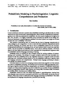
CHR(PRISM)-based Probabilistic Logic Learning - KU Leuven [PDF]

PRISM 4.0: Verification of Probabilistic Real-time Systems

PRISM: Probabilistic Model Checking for Performance and Reliability ...