NIH Public Access Author Manuscript Biomed Eng Lett. Author manuscript; available in PMC 2015 January 06.
NIH-PA Author Manuscript
Published in final edited form as: Biomed Eng Lett. 2014 March ; 4(1): 3–18. doi:10.1007/s13534-014-0121-7.
Model Based Filtered Backprojection Algorithm: A Tutorial Gengsheng L. Zeng Department of Electrical Engineering, Weber State University, Ogden, Utah 84408 USA. Department of Radiology, University of Utah, Salt Lake City, Utah 84108 USA, Tel : +801-626-6864 / Fax : + Gengsheng L. Zeng:
[email protected]
Abstract
NIH-PA Author Manuscript
Purpose—People have been wandering for a long time whether a filtered backprojection (FBP) algorithm is able to incorporate measurement noise in image reconstruction. The purpose of this tutorial is to develop such an FBP algorithm that is able to minimize an objective function with an embedded noise model. Methods—An objective function is first set up to model measurement noise and to enforce some constraints so that the resultant image has some pre-specified properties. An iterative algorithm is used to minimize the objective function, and then the result of the iterative algorithm is converted into the Fourier domain, which in turn leads to an FBP algorithm. The model based FBP algorithm is almost the same as the conventional FBP algorithm, except for the filtering step. Results—The model based FBP algorithm has been applied to low-dose x-ray CT, nuclear medicine, and real-time MRI applications. Compared with the conventional FBP algorithm, the model based FBP algorithm is more effective in reducing noise. Even though an iterative algorithm can achieve the same noise-reducing performance, the model based FBP algorithm is much more computationally efficient.
NIH-PA Author Manuscript
Conclusions—The model based FBP algorithm is an efficient and effective image reconstruction tool. In many applications, it can replace the state-of-the-art iterative algorithms, which usually have a heavy computational cost. The model based FBP algorithm is linear and it has advantages over a nonlinear iterative algorithm in parametric image reconstruction and noise analysis. Keywords Image reconstruction; Tomography; Analytic image reconstruction algorithm; Iterative image reconstruction algorithm
© The Korean Society of Medical & Biological Engineering and Springer 2014 Correspondence to: Gengsheng L. Zeng,
[email protected]. CONFLICT OF INTEREST STATEMENTS Zeng GL declares that s/he has no conflict of interest in relation to the work in this article.
Zeng
Page 2
INTRODUCTION NIH-PA Author Manuscript
Medical imaging uses the principle of tomography to obtain pictures of the internal objects within a patient. X-ray computed tomography (CT), positron emission tomography (PET), and single photon emission computed tomography (SPECT) are the most popular modalities that perform tomography. In layman’s language, tomography is a picture of a cross-section of an object [1, 2]. This cross-sectional picture cannot be directly photographed. If a twodimensional (2D) tomographic image is wanted, one-dimensional (1D) measurements need to be acquired at all directions as shown in Fig. 1. The 1D measurements are often referred to as line integrals, ray sums, and Radon transforms. The 2D image of the object can be recovered if all lines that passing through the object is measured. To form the 2D cross-sectional image from these line integrals is called image reconstruction.
NIH-PA Author Manuscript
The most popular image reconstruction technique is the FBP algorithm, in which a ramp filter is applied to the measurements at each view angle and the filtered data are backprojected into the image domain [3–5]. A ramp filter has a gain that is proportional to the frequency. After ramp filtering, the profile of the measurements at each view is changed such that its frequency components are amplified with a gain that is proportional to its frequency. The backprojection is the action to assign the filtered data value uniformly along the line, along which a line integral was performed, in a manner of line-by-line and view-byview. Another popular image reconstruction technique uses iterative algorithms, in which the image is pixelized [6–10]. Usually an objective function is first set up. By minimizing the objective function, image line integral tries to match the measured line-integral value, and the image tries to satisfy some pre-specified properties. An iterative algorithm is chosen to minimize the objective function.
NIH-PA Author Manuscript
The FBP algorithm is simple and fast, and can be used to reconstruct images in Nuclear Medicine and X-ray CT. However, the FBP algorithm generally produces noisy images. An iterative algorithm (e.g., the iterative Landweber algorithm) can outperform the FBP in terms of noise propagation control. For this reason, the FBP algorithm has gradually been replaced by iterative image reconstruction algorithms. The noise control strategies in an FBP algorithm and in an iterative algorithm are different. Usually, an analytic algorithm controls noise by selecting the filter’s cut-off frequency, while an iterative algorithm can control noise by selecting the iteration number. Another way to control noise in an iterative algorithm is to incorporate the noise model in the objective function and to use priors. As an initial step to improve the noise performance of the FBP algorithm, we link the FBP algorithm with an iterative algorithm. In the next section based on our recent publications [11–17], we will discuss how an FBP algorithm can be used to minimize an objective function.
Biomed Eng Lett. Author manuscript; available in PMC 2015 January 06.
Zeng
Page 3
METHODS NIH-PA Author Manuscript
Objective function setup A typical objective function for image reconstruction can be expressed as
(1)
An equivalent expression of this expression is as follows if the objective function F is to be minimized: (2)
In the context of tomography, A in Eqs. (1) and (2) is the projection matrix, X is the pixelized image array written as a column vector, P is the projection array written as a column vector, and β is a relative weighting factor that adjusts the importance of the Bayesian term βXTRX relative to the fidelity term
, which is defined as
NIH-PA Author Manuscript
(3)
The matrix W is a diagonal noise weighting matrix. A typical way of forming W is to set the ith diagonal element in W to be the reciprocal of the noise variance of the ith projection measurement. The square matrix R in Eqs. (1) and (2) is used to characterize an undesired property that should be suppressed. If one wants to enforce some smoothness in the image so that the reconstruction is not too sensitive to noise, the Bayesian term should be a measure of the non-smoothness of the image. One way to promote the smoothness is to suppress the difference between the central pixel value and its neighbors. A Laplace operator that is the second-order derivative, for example, can be used in the matrix R.
NIH-PA Author Manuscript
The Bayesian term can be arbitrarily chosen by the user, and it does not have to be in for form of βXTRX. For example, if one wants the reconstruction X to look like an image Y, the Bayesian term can be designed as β||X − Y||2. Objective function minimization by the iterative Landweber algorithm The optimization problem Eq. (1) has a quadratic objective function, and almost any optimization algorithm can be used to minimize it. Here we choose the iterative Landweber algorithm to minimize Eq. (1). The Landweber algorithm is expressed as [18]: (4)
where AT is the backprojection matrix of A, X(k) is the estimated image at the kth iteration, and α > 0 is the step size. The working principle of the Landweber algorithm is to move in the downhill direction on the surface of the quadratic objective function in Eq. (1). The Biomed Eng Lett. Author manuscript; available in PMC 2015 January 06.
Zeng
Page 4
downhill direction is the negative of the gradient of F. It can be verified that the negative of the gradient of F is 2[ATW(P − AX) − βRX].
NIH-PA Author Manuscript
This recursive relationship Eq. (4) can be re-written as a non-recursive expression as follows
(5)
In Eq. (5), line 2 is obtained by re-grouping the terms in line 1, and line 3 is obtained by using the relationship X(k+1) = αATWP + (I − αATWA − αβR)X(k) recursively k times, with a decreasing k until k = 0. If the initial image X(0) is selected as zero, the result from k iterations of the Landweber algorithm is
NIH-PA Author Manuscript
(6)
This non-recursive expression Eq. (6) is not in a closed form, meaning that it contains a summation of k terms. Next, we will convert Eq. (6) into a closed form, without the summation of many terms. Recall the summation formula of a geometric series
(7)
In fact, a similar formula exists for matrices [19]. We have
NIH-PA Author Manuscript
(8)
Thus Eq. (6) has a closed form: (9)
The significance of formula Eq. (9) is that a closed-form expression for the results at any iteration is available, and in principle the Landweber result at any specified iteration number can be achieved in one step. This non-iterative expression Eq. (9) of the Landweber algorithm resembles a “backproject first, then filter” algorithm, in the sense that the
Biomed Eng Lett. Author manuscript; available in PMC 2015 January 06.
Zeng
Page 5
projection data P are first backprojected by the operator AT and then filtered by (ATWA + βR)−1[I − (I − αATWA − αβR)k].
NIH-PA Author Manuscript
Fourier domain representation with examples In order to obtain a Fourier domain representation, let us assume a special noise weighting matrix W: The weighting factors for all projections at the same view angle are identical. The noise weighting is thus view based. This view-based weighting assumption will be removed in the latter part of this paper. In tomography, the matrix A is the projection operator and its transposed matrix AT is the backprojector. When the combined matrix ATWA is applied to an image vector X, it first projects X into the projection domain as AX, it then weights the projections at each view with a constant and produces WAX, and finally it backprojects the weighted projections into the image domain as ATWAX.
NIH-PA Author Manuscript
If W is an identity matrix I, ATWA = ATA is a projection operation followed by a backprojection operation. This combined effect of projection/backprojection is to blur the image, and this type of blurring can be effectively removed by using a 2D ramp filter ||ω⃑||. This is the working principle of the “backproject first, then filter” algorithm. Therefore, (ATA)−1 corresponds to ||ω⃑||, and (ATA) corresponds to 1/||ω⃑||. If W represents the view-based weighting, then (ATWA) corresponds to w(θ)/||ω⃑||, where θ is the view angle and w(θ) is the weighting factor in W corresponding to the view angle θ. According to the Central Slice Theorem [1], the view angle θ is the same in the spatial domain and in the Fourier domain. Example 1—In the spatial domain XTRX can be used to extract some unwanted features of the image X. For example, if one wants a minimum norm solution, then R can be chosen as the identity matrix and XTRX = XTX is the norm of the image X. Since RX = X, the Fourier domain’s counterpart of R has the transfer function of 1 (constant one). From the above discussion, we can find the Fourier domain counterpart of the matrix representation (ATWA + βR)−1[I − (I − αATWA − αβR)k] as
NIH-PA Author Manuscript
(10a)
or
(10b)
if a minimum norm Bayesian term is selected. In Algorithm Eq. (9), the portion ATWP is weighted backprojection with a weighting factor w(θ) for angle θ. Therefore, Algorithm Eq.
Biomed Eng Lett. Author manuscript; available in PMC 2015 January 06.
Zeng
Page 6
NIH-PA Author Manuscript
(9) can be implemented by a “backproject first, then filter” algorithm, in which the projection measurements are first backprojected into to image domain without any weights, the 2D ramp filter ||ω⃑|| is then applied to the backprojected image, and finally the image is post-filtered by
(11)
The reader may wonder why the portion ATWP is weighted backprojection, but un-weighted backprojection is used in the first step of the implementation. This is because the weighting factor w(θ) in ATWP is cancelled by the factor 1/w(θ) in Eq. (10b). One observes that the filter Eq. (11) reduce to a constant 1 (that is, “doing nothing”) when β = 0 and k → ∞. Example 2—If one wants to obtain a smooth solution, R can be chosen as the Laplace operator. The Laplace operator in the 2D continuous image domain is defined as
NIH-PA Author Manuscript
(12)
and its matrix representation R is difficult to get if the pixelied image is written as a vector. In actual implementation of any image reconstruction algorithm, the 2D image is always represented by a 2D array (instead of a 1D vector) and thus the Laplace operator has a simple representation as a 2D convolution kernel:
(13)
and its 2D Fourier domain transfer function is ||ω⃑||2. In this particular situation, the Fourier domain counterpart of the matrix representation (ATWA + βR)−1[I − (I − αATWA − αβR)k] is
NIH-PA Author Manuscript
(14a)
or
(14b)
Similar to Example 1, Example 2 can also be implemented in 3 steps: first, unweighted backprojection; second, 2D ramp filtering; third, post-filtering by
Biomed Eng Lett. Author manuscript; available in PMC 2015 January 06.
Zeng
Page 7
NIH-PA Author Manuscript
(15)
The post-filtering transfer function in Eq. (15) reduces to a constant 1 as β = 0 and k → ∞. Example 3—If one wants the reconstructed image X somewhat look like image Y, the objective function can be set up as
(16)
An iterative algorithm can be used to minimize this objective function as an iterative procedure:
(17)
NIH-PA Author Manuscript
Assuming X(0) = 0 and using Eq. (8), Eq. (17) becomes
(18)
The algorithm Eq. (18) in the matrix representation can be readily transformed into a “backproject first, then filter” algorithm as follows: first, backprojecting the measurements; second, scaling the reference image Y by b and adding the resultant image to the backprojected image; third, applying the 2D ramp filter ||ω⃑||; finally, post-filtering the image with the transfer function
(19)
NIH-PA Author Manuscript
The post-filtering transfer function in Eq. (19) reduces to a constant 1 as β = 0 and k → ∞. We must point out that post-filtering can be applied to any images, regardless whether they are reconstructed by the “backproject first, then filter” algorithm, the FBP algorithm, or even iterative algorithms. FBP algorithm with examples In the above derivation, we learn that a quadratic objective function F can be minimized by an iterative algorithm whose updating term is a linear function of the unknown image X. This updating term is proportional to the negative gradient of the objective function F. This iterative algorithm has a closed-form matrix multiplication representation, which can be further transformed into a “backproject first, then filter” algorithm, and the filtration procedure is implemented in the 2D Fourier domain.
Biomed Eng Lett. Author manuscript; available in PMC 2015 January 06.
Zeng
Page 8
NIH-PA Author Manuscript
In tomography, the Central Slice Theorem plays an important roll. It links a 2D object (image) to its 1D projections at various views. This theorem can also transform between an FBP algorithm and a “backproject first, then filter” algorithm. In an FBP algorithm, a 1D ramp filter is first applied to the 1D projections, and then the filtered 1D projections are backprojected into the image domain. On the other hand, in a “backproject first, then filter” algorithm, the 1D projections are first backprojected into the 2D image domain, and then a 2D ramp filter is applied. The relationship between the 2D ramp filter and the 1D ramp filter is that the 1D filter is a central slice of the 2D filter, as shown in Fig. 2. In principle, any “backproject first, then filter” algorithm can be transformed into an FBP algorithm, simply by forming the new 1D filter (at view angle θ) that is the central slice of the 2D filter (at view angle θ) in the “backproject first, then filter.” If the 2D filter is isotropic, the 1D filter is the same for all views. We will illustrate how this can be done by using the three examples that we saw earlier in this paper. Example 1—In transforming a “backproject first, then filter” algorithm into an FBP algorithm, the 2D ramp filter is replaced by a 1D ramp filter, and the post-filter defined in Eq. (11) is replaced the 1D pre-filter
NIH-PA Author Manuscript
(20)
which is applied to the raw projections at the same time as the 1D ramp filter is applied, at view angle θ. Example 2—The 2D post-filter defined in Eq. (15) is replaced the 1D pre-filter at view angle θ:
(21)
Example 3—The 1D pre-filter in this case is simple, by replacing ||ω⃑|| with |ω| in (19) as
NIH-PA Author Manuscript
(22)
However, the portion (ATP + βY) in Eq. (18) must also be properly modified to fit the FBP algorithm so that Y is in the form of “ATQ” that is the backprojection of a certain set of projections Q. Let Y = ATQ, where Q can be obtained as: first forward project the reference image, and then apply the 1D ramp filter to the pseudo projections. In other words, Q is a set of the ramp filtered projections of the reference image Y. If we denote the measured projections of a 2D object as P, the proposed FBP algorithm will require the forming of new projection data set: P + βQ. The new FBP algorithm for this case consists of the following steps: filtering the
Biomed Eng Lett. Author manuscript; available in PMC 2015 January 06.
Zeng
Page 9
data set P + βQ with the ramp filter modified by the window function in Eq. (22); performing the conventional backprojection.
NIH-PA Author Manuscript
Ray-by-ray noise weighting in an FBP algorithm The FBP algorithms developed so far can only incorporate with a view-based noise model. In other words, the noise weighting function w(θ) has been assumed to be a function of the view angle θ. Next, using Example 1, we will extend the view-by-view noise weighting to ray-by-ray noise weighting in an ad hoc manner. For the ray-based noise weighting, w is a function of the ray: w = w(ray). A popular approach to assigning the weighting factor is to let w(ray) be proportional to the reciprocal of the noise variance of the ray measurement. From now on, we will combine the ramp filter |ω| and the window function in Eq. (20). At each view angle, we quantize the ray-based weighting function into N+1 values: w0, w1, …, wN, which in turn give N+1 different filters. They are
NIH-PA Author Manuscript
(23)
for n = 0, 1, 2, …, N. Using these N+1 filters, N+1 sets of filtered projections are obtained. Before backprojection, one of these N+1 projections is selected for each ray according to its proper weighting function. Only one backprojection is performed using the selected filtered projections.
NIH-PA Author Manuscript
More expressively, let us assume N be 10 and the measurements be transmission data. The noise model for the transmission data will be discussed in the later part of this paper. Before the projections data are ready to process, form 10 Fourier domain filter transfer functions Hk,α,β,wn(ω) as defined in Eq. (23) with wn = exp(−0.1 · n · pmax), n = 0, 1, 2, …, 10, respectively. Here pmax is the maximum value of the measured line integrals. Note: In implementation, ω is a discrete frequency index and takes the discrete values of between 0 and 0.5 (which corresponds to the highest frequency before sampling). The FBP algorithm for the case of Example 1 can be implemented as Step 1: At each view angle θ, find the 1D Fourier transform of p(t, θ) with respect to t, obtaining P(ω, θ). Step 2: Form 11 versions of P̂n(ω, θ) = P(ω, θ) · Hk,α,β,wn(ω) with n=0, 1, …, 10. Step 3: Take the 1D inverse Fourier transform of P̂n(ω, θ) with respect to ω, obtaining p̂n(t, θ) with n=0, 1, …, 10. Step 4: Construct p̂(t, θ) by letting p̂(t, θ) = p̂n(t, θ) if p(t, θ) ≈ 0.1 · n · pmax. Step 5: Backproject p̂(t, θ) to obtain the final image.
Biomed Eng Lett. Author manuscript; available in PMC 2015 January 06.
Zeng
Page 10
The FBP algorithm with spatial domain filtering
NIH-PA Author Manuscript
Both of the conventional FBP algorithm and the new FBP algorithm with view-based noise weighting have a shift-invariant property. This property allows the filtering procedure to be efficiently implemented as multiplication in the Fourier domain or as convolution in the spatial domain. It is well known that Fourier-domain multiplication is equivalent to spatialdomain convolution. In principle, any FBP algorithm with Fourier-domain filtering can find its equivalent FBP algorithm that performs filtering in the spatial domain as convolution, if the convolution kernel can be readily obtained. After the ray-based noise model is adopted, the noise weighted FBP algorithm no longer has the shift-invariant property. If the filtering procedure is to be implemented in the Fourier domain, multiple versions of the filtered projections must be generated as discussed above, where the projection data at each view must be filtered multiple times (say, 11 times).
NIH-PA Author Manuscript
It is well known that using fast Fourier transform (FFT) and inverse Fourier transform (IFFT) to implement convolution is more computationally efficient than calculating convolution directly in the spatial domain. Let the detector size be N. If the filter is shift invariant, the spatial domain convolution takes O(N2) arithmetical operations, while the FFT/IFFT method can perform it with O(N log N) operations. However, if the filter is shift variant, the spatial domain implementation still takes O(N2) arithmetical operations, while the FFT/IFFT method computes it using O(N2 log N) operations. Without using the quantization method, one would use 1024 filters to filter the projections 1024 times, if there were 1024 detection channels (or detection cells) on the detector. Therefore, it is not efficient to perform filtering in the Fourier domain if the filter is shift variant and the quantization method is not adopted. On the other hand, it is more efficient if filtering is implemented in the spatial domain as integration when the kernel is spatially varying. If the integration kernel has a closed-form expression, the computation cost for spatial-domain filtering is the same as that of convolution, both using a dot product for implementation.
NIH-PA Author Manuscript
Next, we will investigate how to implement the ray-based, noise-weighted FBP algorithm in the form of “convolution” backprojection. However, this “convolution” is not a true convolution operation, because the integration kernel varies from ray-to-ray according to the noise variance of the projection ray. An expansion method will be suggested to obtain a closed-form integration kernel so that the “convolution” can be computed efficiently. In order to have a spatial domain filter, all we need is an integration kernel. We will find such a kernel using Example 1. A routine method to find a discrete filter kernel hw(n) is to evaluate the following integral [1], which is the 1D inverse Fourier transform of the transfer function defined in Eq. (23) with k → ∞:
(24)
Biomed Eng Lett. Author manuscript; available in PMC 2015 January 06.
Zeng
Page 11
where we used the property that the transfer function Hw(ω) is an even function. It is unlikely that the integral in Eq. (24) has an explicit closed-form expression.
NIH-PA Author Manuscript
Our method is to find a finite expansion of the function Hw(ω) and the expansion should have closed-form inverse Fourier transform. Since 1 / (1 + β0ω) with β0 > 0 is a monotonically decreasing function on [0, 1/2], we have decided to use the following approximation: (25)
where the parameters β1 and β2 are to be determined. The range of ω is [0, 1/2]. The approximation Eq. (25) is already exact at ω = 0. We further request that Eq. (25) to be exact at ω = 1/4 and ω = 1/2. Thus, we have two unknowns (β1 and β2) and two equations: (26)
NIH-PA Author Manuscript
(27)
Solving these two equations yields
(28)
where
(29)
NIH-PA Author Manuscript
Using the above results and an integral table, the closed-form filter kernel Eq. (24) can be obtained as (n ≠ 0):
(30)
and
(31)
Biomed Eng Lett. Author manuscript; available in PMC 2015 January 06.
Zeng
Page 12
The purpose of Eq. (31) is to guarantee that Hw(0) = 0. The filter kernel hw(n) is an even function with respect to index n.
NIH-PA Author Manuscript
If we take the limit of β → 0, Eq. (30) reduces to
(32)
which is the well-known convolution kernel for the conventional ramp filter. It is worth mentioning that the method to obtain Eq. (30) is suitable for the parallel-beam or flat-detector fan-beam imaging geometries. For the curved-detector fan-beam imaging geometry, its convolution kernel hcurve(n) is a scaled version of the parallel-beam or the flatdetector fan-beam geometry’s convolution kernel h(n) [1]
(33)
NIH-PA Author Manuscript
where D is the fan-beam focal length. Applying the curved-detector fan-beam relationship Eq. (33) to kernel Eq. (30) yields
(34)
Implementation procedure of the ray-weighted FBP algorithm with spatial domain filtering
NIH-PA Author Manuscript
Like the conventional convolution backprojection FBP algorithm, the first step in the implementation first it to filter the projections with a spatially variant, noise weighted, ramp filter, and the filtering is performed in the spatial domain by evaluating a dot product. The filtered data are then backprojected into the image domain. Since the backprojection procedure of our algorithm is identical to the conventional backprojection, we only discuss the discrete implementation of the filtering procedure below. We denote the discretely sampled projections as pd(n, m), where n is the index on the detector and m is the index of the view angle. We use a subscript d to indicate discretely sampled functions. For any fixed view angle m, do the following: Loop through the detector cell index n: Step 1: Consider the noise model of pd(n, m) and estimate the variance of the measurement pd(n, m). Let the weighting factor wd(n, m) be the reciprocal of the variance (or a function of the variance). Step 2: Evaluate the spatial-domain filter kernel hw(n) according to Eqs. (30) and (31). Step 3: Calculate filtered projection value qd(n, m) using a dot product: Biomed Eng Lett. Author manuscript; available in PMC 2015 January 06.
Zeng
Page 13
(35)
NIH-PA Author Manuscript
Noise models and parameter selection Emission tomography—In model based emission tomography, the measured projections are assumed to be suffered from the Poisson noise, assuming the variance to be the same as the mean. For emission data the ray-based noise weighting factor w can be set as 1/variance, which is 1/projection. There is no right way or wrong way in noise modeling. The users should experiment some different noise weighting strategies and select the best one for their applications. One can feel free to choose the noise weighting factor w as 1/(projection)0.5 or 1/(projection) 0.3 if they give better results than 1/projection, and in some applications they do. The choice of the weighting factor w as 1/variance does not always gives the optimal results. Transmission tomography—In transmission tomography, the projections are related to the number of entering photons, Nin, and departing photons, Nout, according to Beer’s law:
NIH-PA Author Manuscript
(36)
where Nin is assumed to be a constant and Nout is assumed to be corrupted with the Poisson noise. The variance of the projection is approximately 1/(Nout = 1/(Nine−projection). Therefore, the noise weighting factor can be chosen to proportional to e−projection. The users have the freedom to chose the weighting factor as e−0.5 × projection or e−0.3 × projection, etc, if better results can be obtained. Selection of β and weights w—The model based FBP algorithm’s filter kernel depends either on the “iteration number” k or β0 = β/w which in turn depends on the Bayesian term control parameter β and the current ray weighting factor w. It may depend on both k and β0. One can let k → ∞ and only use a non-zero parameter β. We must point out that if one simultaneously lets k → ∞ and β = 0, the noise weighting w is not effective.
NIH-PA Author Manuscript
The principle of selecting both β and w is exactly the same for both of the Fourier-domain implementation and spatial-domain implementation. Both methods can use the same β and w values. There is a trade-off consideration for the objective function in Eq. (1). A larger β value emphasizes the regularization Bayesian term more, and usually encourages a smoother image with a lower image resolution. Setting β to zero or an extremely small positive value results in a high resolution but noisy image. The FBP algorithm is somewhat equivalent to an iterative algorithm with an iteration number of infinity (if we ignore the pixelization effect in the iterative algorithm). Also, the noise weighting is always relative. By “relative” we mean that the projection rays compete with each other, and some rays are emphasized while others are de-emphasized by assigning a set of weights, one for each ray. The weights are also relative, meaning that you can scale the weights by a constant value. However, this scaling value affects the selection of the value of β. Usually, the weights w are selected as
Biomed Eng Lett. Author manuscript; available in PMC 2015 January 06.
Zeng
Page 14
the reciprocal of the noise variance (or a function of the variance) of projection value of the associated ray.
NIH-PA Author Manuscript
One may argue that in an iterative algorithm the noise weighting is always effective, regardless whether there is a Bayesian term or not. When a system of linear equations is not consistent due to noise, noise weighting is commonly used to define an acceptable “solution.” When a linear system has a unique solution, the noise weighting should not affect the final (unique) solution. However, an iterative algorithm can only present a result with a finite number of iterations. Even though the final solution is unique, the noise weighting can alter the path towards to unique solution. Because the final solution is usually very noisy, early algorithm termination is the most common method of regularization. The effects of multiple convergent paths and early termination make the noise weighting effective in an iterative algorithm, regardless whether there is an explicit Bayesian regularization term or not. An effective regularization is always applied in one way or another.
RESULTS NIH-PA Author Manuscript
The effect of the iteration number k\ In this part, we compare the effect of the iteration number k on the iterative Landweber algorithm and the new analytic FBP algorithm with a modified ramp filter Eq. (23) with β = 0 and w = 1. In this simple comparison study, we removed the Bayesian term (by setting β = 0) and noise weighting (by setting w = 1). We selected the step size α for the iterative Landweber algorithm and the new FBP algorithm, separately, by trial-and-error so that these two algorithms could produce similar images for the same “iterative number” k. The Shepp-Logan head phantom [3] was used in computer simulation studies. A 1D parallel-hole detector was rotated over 180° with 120 views and 128 detector bins on the detector. The images were reconstructed in a 256×256 array, and the central 128×128 array was used for image display. Poisson noise was added to the projection data before image reconstruction. Two algorithms were used for image reconstruction: the iterative Landweber algorithm with α=0.5×0.0000525 and the new FBP algorithm with Eq. (23) as the frequency-domain window function and α=0.5.
NIH-PA Author Manuscript
Some computer simulation results are shown in Figs. 3 and 4, where each image is displayed from its minimum image pixel value (black) to its maximum image pixel value (white). No post processing of the images was performed. The negative values in the images were not altered. Images in Fig. 3 used noiseless projections, and they are used to illustrate the resolution improvement as the index k gets larger. The profiles are drawn horizontally at the center of the images. The images are almost converged when k = 200. With the same index k, the iterative Landweber algorithm and the windowed FBP algorithm give almost the same resolution.
Biomed Eng Lett. Author manuscript; available in PMC 2015 January 06.
Zeng
Page 15
NIH-PA Author Manuscript
In Fig. 4, Poisson noise was added to the projections. The average total count in the projections was 792500 for each noise trial. Typical reconstructions are displayed in the left 2 columns. As the index k increases, the resolution improves, but the noise is more amplified. Signal-to-noise (S/N) ratio images were obtained by using 100 noise realizations and are displayed in the 3rd and 4th columns. In the S/N image each pixel represents the ratio of the mean value over the standard deviation. The S/N was calculated pixel-wise using the following formula:
(37)
where n is the index of the noise realization.
NIH-PA Author Manuscript
As shown by the line profiles drawn horizontally across at the center of the S/N images, the iterative Landweber algorithm and the new FBP algorithm have almost the same noise property for the same index k. It is interesting to notice that when the algorithms are almost converged at k = 200, the S/N image is very similar to the density image itself. The effect of the Bayesian term (β) When β ≠ 0 in the objective function (1), its associated optimization algorithms are called the maximum a posteriori (MAP) algorithms. The results from both the iterative MAP algorithm and the new FBP-MAP algorithm are compared, using the same parameter β (=0.1 and 0.3) and the same iteration indices k = 2, 20, and 200, respectively. The requirement of choosing parameter α is that α/|ω| ≤ 1 in the newly developed FBP-MAP algorithm and α · wview/|ω| ≤ 1 in the newly developed noise variance weighted FBP algorithm, where wview is a noise weighting factor. In order to use the same parameter α=0.5, we scaled the iterative algorithm’s projection/backprojection operator ATA by 0.00005, that is,
(38)
In Eq. (38), R was chosen as the Laplacian, whose convolution kernel is {−0.5, 1, −0.5}.
NIH-PA Author Manuscript
Computer simulation results are shown in Figs. 6–8. Each image is displayed from its minimum image pixel value (black) to its maximum image pixel value (white). No post processing of the images was performed. The negative values in the images were not altered. Images in Figs. 5 and 6 I used noiseless projections, and they are used to illustrate the resolution improvement as the index k gets larger. The profiles are drawn horizontally at the center of the images. The images almost converge when k = 200. From the profiles, one can tell that a larger β value makes the image smoother. With the same index k, the iterative Landweber MAP algorithm and the windowed FBP algorithm give almost the same resolution.
Biomed Eng Lett. Author manuscript; available in PMC 2015 January 06.
Zeng
Page 16
NIH-PA Author Manuscript
In Figs. 7–9, Poisson noise was added to the projections. Typical reconstructions are displayed in the rows 2 and 3. As the index k increases, the resolution improves, but the noise is amplified. S/N ratio images were obtained by using 100 noise realizations and are displayed in the 4th and 5th rows. In the S/N image each pixel represents the ratio of the mean value over the standard deviation. As shown by the line profiles drawn horizontally across at the center of the S/N images, the iterative Landweber MAP algorithm and the proposed FBP algorithm have almost the same noise property for the same index k. Low-dose x-ray CT results Fig. 9a shows the conventional cone-beam FBP Feldkamp’s [20] reconstruction of a transverse slice in the abdominal region of a cadaver. This study used low dose. The cadaver arms were outside the display field of view; the arms further attenuated the x-rays, creating streak artifacts in the middle of the image from left-to-right across the torso. Fig. 9b shows the new FBP’s reconstruction, with β = 2.6×10⁻⁵, k = ∞, and w = e−p. The ray-based noise weighting in the new FBP algorithm effectively removes the streaking artifacts that appear in Fig. 9a. The images are displayed from −400 HU to 400 HU.
NIH-PA Author Manuscript
Results with spatial-domain implementation of the weighted ramp filter Fig. 10 shows the results of the FBP reconstructions with spatial-domain implementation of the windowed ramp filter: Fig. 10a without noise weighting and Fig. 10b with noise weighting. Fig. 10c is the gold standard image, which is the conventional fan-beam convolution backprojection reconstruction using the standard dose CT data. The tube voltage was 120 kV and current was 500 mA. Real time MRI
NIH-PA Author Manuscript
To illustrate the feasibility of the new FBP-MAP algorithm in a real-time magnetic resonance imaging (MRI), a human cardiac perfusion study was used [21]. The MRI data were acquired with a Siemens 3T Trio scanner, using phased array of coils, one of which was chosen to demonstrate the proposed method. The scanner parameters for the radial acquisition were TR = 2.6 msec, TE = 1.1 msec, flip angle = 12°, Gd dose = 0.03 mmol/kg, and slice thickness = 6 mm. Reconstruction pixel size was 1.8 × 1.8 mm2. Each image was acquired in a 62 msec readout. The acquisition matrix size for an image frame was 256 × 24, and 60 sequential images were obtained at 60 different times. At each time frame, the kspace is sampled with 24 uniformly spaced radial lines over an angular range of 180°; however, the 24-line sampling patterns of the adjacent time frames are offset by 180°/96. If one sums up the measurements from temporally adjacent 4 time frames, the k-space will have a 96-line sampling pattern, uniformly distributed over an angular range of 180°. In our image reconstruction method, each time frame requires current 24-line measurement P and associated time-averaged 96-line measurement P̂, which uses the measurements from the current 24-line data, two “immediately after” 24-line measurements, and two “immediately before” 24-line measurements. A symbolic expression for P̂ is given as: (39)
Biomed Eng Lett. Author manuscript; available in PMC 2015 January 06.
Zeng
Page 17
NIH-PA Author Manuscript
The fact that one image was acquired with 24 views (i.e., 24 radial lines in the k-space) makes the k-space undersampled. In cardiac imaging, the object is in constant motion. The number of time frames to be used in the secondary data set P̂ should be as small as possible while still cover as much the k-space as possible. In our example, there are 96 possible radial k-space lines and each time frame measures 24 of those lines. That is, 4 total time frames are required to cover the 96 lines. In addition to the current measurement, the secondary data set needs additional data from other 3 time frames. In order to balance the “before” and “after” time frames, we chose two “immediate before” time frames and two “immediate after” time frames. Both the conventional FBP algorithm and the proposed non-iterative FBP-MAP algorithm were used to reconstruct the images. In our MRI data acquisition, each k-space radial readout had 256 samples. After zero-padding, the length N was chosen as 1024, and the frequency variable ω took discrete values of 2πn/N, for integers n. Parameter β was chosen as 0.07, which was selected by experience and the noise level of a data set. Parameter β controls the influence of the reference image, and β=0 implies that the reference image is not used.
NIH-PA Author Manuscript
Fig. 11 shows the reconstruction results from the undersampled MRI data using both conventional FBP algorithm and the new FBP-MAP algorithm. The images obtained by the convention method (see the 1st row of Fig. 11) suffer from severe angular aliasing artifacts and are noisy. The angular aliasing artifacts are significantly reduced and the noise is suppressed in the images obtained by the new FBP-MAP method (see the 2nd row of Fig. 11). There are 60 time frames in the study, and results form a subset of 6 time frames are shown in Fig. 11, and the time spacing is 10 time frames. Due to the nature of dynamic imaging, the image intensity of a series of image changes over time. In order to view each individual reconstruction properly, each image in the 1st and 2nd rows is displayed from zero to its maximum value.
NIH-PA Author Manuscript
The 3rd row of Fig. 11 shows the difference between the 1st row and the 2nd row. The purpose of the difference image is to check whether the constrained reconstruction is able to track the dynamic changes and shapes overtime. The images in the 3rd row are obtained as follows. Both of the FBP images and FBP-MAP images are first normalized. If one treats the time as the third dimension, the normalization procedure is three-dimensional, with the first two dimensions as spatial and the third dimension as temporal. The normalized “3D” FBP image has a maximum value of unity and so does the normalized “3D” FBP-MAP image. The “3D” difference image is calculated as the normalized FBP image minus the normalized FBP-MAP image. The difference image for all time frames is displayed using a common gray-scale interval of [−0.2, 0.2] in the 3rd row of Fig. 11. In the cardiac region, the difference image is almost zero, implying that the constrained reconstruction faithfully follows the intensity change and the cardiac motion as represented by the FBP reconstruction.
Biomed Eng Lett. Author manuscript; available in PMC 2015 January 06.
Zeng
Page 18
CONCLUSIONS NIH-PA Author Manuscript
It was believed for a long time that the FBP algorithm was unable to incorporate the projection data’s noise model during image reconstruction. Recently, a noise-weighted FBP algorithm was developed, which is able to minimize a quadratic objection function that can contain a Bayesian term. This tutorial paper reviews this new technology. Like all other model based algorithm, the new FBP algorithm minimized an objective function. The resultant FBP algorithm is almost the same as the conventional FBP algorithm, except that the ramp filter is modified by a window function. This window function depends on the noise weighting and Bayesian term information. Intuitively speaking, the filter has a narrower lowpass-type window function if the data are noisier. If the noise weighting is a function of the view angle, the FBP algorithm is shift invariant, and the modified ramp filter can be implemented either as a Fourier domain multiplication or as a spatial domain convolution.
NIH-PA Author Manuscript
If the noise weighting is a function of the projection ray, the FBP algorithm is shift variant, and the modified ramp filter can be implemented either as multiple Fourier domain multiplications or as a spatial domain dot product. We must point out that it is not a straightforward task to obtain a closed-form spatial domain filter kernel. We have presented some computer simulations to illustrate the equivalence of an iterative Landweber algorithm and the new FBP algorithm. For the same “iterative number” k, they provided comparable images. The effectiveness of the noise weighting has been demonstrated by a low-dose x-ray CT study using clinical cadaver data. The severe streaking artifacts appeared in the conventional FBP reconstruction, while they were successfully removed with the noise weighting. We must be caution that noise weighting is not a silver bullet. If the noise is extremely large, noise weighting is not effective and it only results in a low-resolution image. Finally, we applied the new FBP algorithm to a set of real-time MRI data. This MRI study demonstrated the power of a Bayesian constraint that encourages the reconstructed image to look like a reference image. No noise weighting was used in this MRI study.
NIH-PA Author Manuscript
The main advantage of the new model based FBP algorithm is its computational efficiency (fast). Its computation time is almost the same as that of the conventional FBP algorithm. Another advantage of the new FBP algorithm is the linearity property. One can readily obtain a noise variance image for any given data set. This feature is attractive in parametric imaging, where some parameters and their uncertainties are to be estimated.
Acknowledgments He also thanks Raoul M. S. Joemai of Leiden University Medical Center for collecting and providing raw data of the cadaver CT scan, and Edward DiBella of University of Utah for providing raw MRI cardiac data. He thanks “International Journal of Imaging Systems and Technology” for their permission to re-use Fig. 11 in this paper and “Medical Physics” the permission to re-use Figs. 3–10 in this paper.
Biomed Eng Lett. Author manuscript; available in PMC 2015 January 06.
Zeng
Page 19
References NIH-PA Author Manuscript NIH-PA Author Manuscript NIH-PA Author Manuscript
1. Zeng, GL. Medical Image Reconstruction, A Conceptual Tutorial. 1. Beijing: Springer; 2010. 2. Kak, AC.; Slaney, M. Principles of Computerized Tomographic Imaging. IEEE Press; 1988. 3. Shepp LA, Logan BF. The Fourier reconstruction of a head section. IEEE T Nucl Sci. 1974; 21(3): 21–43. 4. Radon J. Über die bestimmung von funktionen durch ihre integralwerte längs gewisser mannigfaltigkeiten. Ber Verh Sächs Akad Wiss Leipzig Math Nat. 1917:262–77. kl 69. 5. Bracewell RN. Strip integration in radio astronomy. Aust J Phys. 1956; 9:198–217. 6. Geman S, McClure DE. Statistical methods for tomographic image reconstruction. Conf Proc Session Int Stat Inst. 1987; LII-4:5–21. 7. Dempster AP, Laird NM, Rubin DB. Maximum likelihood from incomplete data via the EM algorithm. J R Stat Soc Series B. 1977; 39(1):1–38. 8. Shepp LA, Vardi Y. Maximum likelihood reconstruction for emission tomography. IEEE T Med Imaging. 1982; 1(2):113–22. 9. Hudson HM, Larkin RS. Accelerated image reconstruction using ordered subsets of projection data. IEEE T Med Imaging. 1994; 13(4):601–9. 10. Lange K, Carson R. EM reconstruction algorithms for emission and transmission tomography. J Comput Assist Tomogr. 1984; 8(2):302–16. 11. Zeng GL. A filtered backprojection algorithm with characteristics of the iterative Landweber algorithm. Med Phys. 2012; 39(2):603–7. [PubMed: 22320769] 12. Zeng GL. A filtered backprojection MAP algorithm with non-uniform sampling and noise modeling. Med Phys. 2012; 39(4):2170–8. [PubMed: 22482638] 13. Zeng GL. Filtered backprojection algorithm can outperform maximum likelihood EM algorithm. Int J Imag Syst Tech. 2012; 22(2):114–20. 14. Zeng GL, Li Y, DiBella ERV. Non-iterative reconstruction with a prior for undersampled radial MRI data. Int J Imag Syst Tech. 2013; 23(1):53–8. 15. Zeng GL, Zamyatin A. A filtered backprojection algorithm with ray-by-ray noise weighting. Med Phys. 2013; 40:031113. http://dx.doi.org/10.1118/1.4790696. [PubMed: 23464293] 16. Zeng GL, Li Y, Zamyatin A. Iterative total-variation reconstruction vs. weighted filteredbackprojection reconstruction with edge-preserving filtering. Phys Med Biol. 2013; 58(10):3413– 31. [PubMed: 23618896] 17. Zeng GL. Noise weighted FBP algorithm versus ML-EM algorithm. J Nucl Med Technol. 2013; 41(4):283–8. [PubMed: 24159012] 18. Strand ON. Theory and methods related to the singular-function expansion and Landweber’s iteration for integral equations of the first kind. SIAM J Numer Anal. 1974; 11(4):798–825. 19. Schafer RW, Mersereau RM, Richards MA. Constrained iterative restoration algorithms. Proc IEEE. 1981; 69(4):432–50. 20. Feldkamp LA, Davis LC, Kress JW. Practical cone beam algorithm. J Opt Soc Am A. 1984; 1(6): 612–9. 21. Adluru G, McGann C, Speier P, Kholmovski EG, Shaaban A, DiBella EVR. Acquisition and reconstruction of undersampled radial data for myocardial perfusion MRI. J Magn Reson Imaging. 2009; 29(2):466–73. [PubMed: 19161204]
Biomed Eng Lett. Author manuscript; available in PMC 2015 January 06.
Zeng
Page 20
NIH-PA Author Manuscript Fig. 1.
NIH-PA Author Manuscript
Line integral measurements are acquired for all directions to order to obtain a 2D tomographic image.
NIH-PA Author Manuscript Biomed Eng Lett. Author manuscript; available in PMC 2015 January 06.
Zeng
Page 21
NIH-PA Author Manuscript Fig. 2.
NIH-PA Author Manuscript
The 1D ramp filter is a central slice of the 2D ramp filter.
NIH-PA Author Manuscript Biomed Eng Lett. Author manuscript; available in PMC 2015 January 06.
Zeng
Page 22
NIH-PA Author Manuscript NIH-PA Author Manuscript
Fig. 3.
Comparison studies of the iterative Landweber algorithm and the windowed FBP algorithm. Noiseless data are used. The goal is to compare the image resolution for different index k.
NIH-PA Author Manuscript Biomed Eng Lett. Author manuscript; available in PMC 2015 January 06.
Zeng
Page 23
NIH-PA Author Manuscript NIH-PA Author Manuscript
Fig. 4.
Comparison studies of the iterative Landweber algorithm and the windowed FBP algorithm. Noisey data are used. The goal is to compare the image noise for different index k. The S/N ratio images use 100 noise realizations.
NIH-PA Author Manuscript Biomed Eng Lett. Author manuscript; available in PMC 2015 January 06.
Zeng
Page 24
NIH-PA Author Manuscript Fig. 5.
NIH-PA Author Manuscript
Iterative MAP vs. FBP-MAP with β = 0.1 (i.e., small Bayesian term weighting) using noiseless data.
NIH-PA Author Manuscript Biomed Eng Lett. Author manuscript; available in PMC 2015 January 06.
Zeng
Page 25
NIH-PA Author Manuscript Fig. 6.
Iterative MAP vs. FBP-MAP with β = 0.3 using noiseless data.
NIH-PA Author Manuscript NIH-PA Author Manuscript Biomed Eng Lett. Author manuscript; available in PMC 2015 January 06.
Zeng
Page 26
NIH-PA Author Manuscript NIH-PA Author Manuscript
Fig. 7.
Iterative MAP vs. FBP-MAP with β = 0.1 (i.e., small Bayesian term weighting) using noisy data.
NIH-PA Author Manuscript Biomed Eng Lett. Author manuscript; available in PMC 2015 January 06.
Zeng
Page 27
NIH-PA Author Manuscript NIH-PA Author Manuscript
Fig. 8.
Iterative MAP vs. FBP-MAP with β = 0.3 using noisy data.
NIH-PA Author Manuscript Biomed Eng Lett. Author manuscript; available in PMC 2015 January 06.
Zeng
Page 28
NIH-PA Author Manuscript
Fig. 9.
Reconstruction results for the clinical cadaver data: (a) The conventional FBP reconstruction, (b) The ray-base-weighted FBP reconstruction. Display window is from −400 HU to 400 HU.
NIH-PA Author Manuscript NIH-PA Author Manuscript Biomed Eng Lett. Author manuscript; available in PMC 2015 January 06.
Zeng
Page 29
NIH-PA Author Manuscript NIH-PA Author Manuscript NIH-PA Author Manuscript
Fig. 10.
Images reconstructed using low-dose CT clinical cadaver data. (a) Conventional convolution backprojection reconstruction. (b) Proposed noise-weighted FBP reconstruction with spatialdomain filtering. (c) Gold-standard: conventional convolution backprojection reconstruction using regular dose CT data.
Biomed Eng Lett. Author manuscript; available in PMC 2015 January 06.
Zeng
Page 30
NIH-PA Author Manuscript Fig. 11.
NIH-PA Author Manuscript
Comparison of conventional FBP reconstruction (1st row) and proposed FBP-MAP reconstruction (2nd row), using undersampled dynamic MRI data. The 3rd row shows the difference images between the 1st and 2nd rows. Six time frames are shown from left to right.
NIH-PA Author Manuscript Biomed Eng Lett. Author manuscript; available in PMC 2015 January 06.