NMR Quantum Computing - Semantic Scholar

NMR Quantum Computing Zhigang Zhang1 , Goong Chen2 , Zijian Diao3 , Philip R. Hemmer4 1

2

3

4

Department of Mathematics, Texas A&M University, College Station, TX 77843 [email protected] Department of Mathematics, Texas A&M University, College Station, TX 77843 [email protected] Department of Mathematics, Ohio University - Eastern, St. Clairsville, OH 43950 [email protected] Department of Electrical and Computer Engineering, Texas A&M University, College Station, TX 77843 [email protected]

ABSTRACT Quantum computing is at the forefront of the scientific and technological research and development of the 21st century. NMR quantum computing is one the most mature technologies for implementing quantum computation. It utilizes the motion of spins of nuclei in custom-designed molecules manipulated by RF pulses. The motion is on a nano- or microscopic scale governed by the Schrödinger equation in quantum mechanics. In this article, we explain the basic ideas and principles of NMR quantum computing, including basic atomic physics, NMR quantum gates and operations. New progress in optically addressed solid state NMR is expounded. Examples of the Shor’s algorithm for factorization of composite integers and quantum lattice-gas algorithm for the diffusion partial differential equation are also illustrated.

1 Nuclear magnetic resonance Many articles in this book are concerned with mathematical problems in mechanics–elasticity, fluid mechanics, materials, etc., which are of the macroscale. At the other extreme is the study of problems in atoms and molecules, photonics, nanotechnology, etc., which are of the micro- or nano-scale governed chiefly by the Schrödinger equation. This area has undergone rapid advancements during the past ten years, in large part due to the stimuli from laser applications, quantum computing and quantum technology, and nanoelectronics. Most of the practitioners in this area are physicists and it appears that this area has not drawn enough attention from mathematicians. Here,

2

Zhigang Zhang, Goong Chen, Zijian Diao, Philip R. Hemmer

we wish to describe one of such developments, namely, nuclear magnetic resonance (NMR) quantum computing. There already exist many papers on this topic, see, e.g., [16, 17, 14, 55, 52, 107], written by physicists and computer scientists. Our chapter here describes the same interest, but perhaps from a more mathematical point of view. 1.1 Introduction As of today, NMR is the most mature technology for the implementation of quantum computing. Naturally, this area is rife with papers. A good internet resource for looking up NMR quantum computing references, both old and new, is the U.S. Los Alamos National Laboratory’s web site http://xxx.lanl.gov/quant-ph. At present, several types of elementary quantum computing devices have been developed, based on AMO (atomic, molecular and optical) or semiconductor physics and technologies. We may roughly classify them into the following: atomic — ion and atom traps, cavity QED; molecular — NMR; semiconductor — coupled quantum dots [11], silicon (Kane) [57]; crystal structure — nitrogen-vacancy (NV) diamond (see Section 3); superconductivity — SQUID. The above classification is not totally rigorous as new types of devices, such as quantum dots, or ion traps imbedded in cavity-QED, have emerged which are of the hybrid nature. Also, laser pulse control, which is of the optical nature, seems to be omnipresent. In [3], a total of 12 types of quantum computing proposals have been listed5 . Nevertheless, it is clear that NMR quantum computing belongs to the class of molecular computing where we use molecules as a small computer. The logic bits are the nuclear spins of atoms in custom designed molecules. Spin flips are achieved through the application of radio-frequency (RF) fields on resonance at the nuclear spin frequencies. The system can be initialized by cooling the system down to the ground state or known low-entropy state, or using a special technology called averaging, especially for liquid NMR working in room temperature. Measurement or readout is carried out by measuring the magnetic induction signal generated by the precessing spin on the receiver coil. Numerous experiments have been successfully tried for different algorithms, mostly using liquid NMR technology. The algorithms tested include Grover’s search algorithm [106, 52, 44, 120], other generalized search algorithms [73], quantum Fourier transforms [24, 112], Shor’s algorithm [109], Deutsch-Jozsa algorithm [13, 71, 25, 82, 22], order finding [105, 98], error correcting code [63], and dense coding [31]. There are 5

The additional proposals not listed above but given in [3] are quantum Hall qubits, electrons in liquid helium, and spin spectroscopies.

NMR Quantum Computing

3

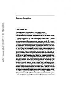
also other implementations reported like cat-code benchmark [62], information teleportation [85] and quantum system simulation [96]. NMR is an important tool in chemistry which has been in use for the determination of molecular structure and composition of solids, liquid and gases since the mid 1940s, by research groups in Stanford and MIT independently, led by F. Bloch and E.M. Purcell, both of whom shared the Nobel prize in physics in 1952 for the discovery. There are many excellent monographs on NMR [29, 89, 79]. There are also many other nice internet website resources offering concise but highly useful information about NMR; cf., e.g., [26, 49, 113]. Let us briefly explain the physics of NMR by following Edwards [26]. The NMR phenomenon is based on the fact that the spin of nuclei of atoms have magnetic properties that can be utilized to yield chemical, physical, and biological information. Through the famous Stern-Gerlach experiment in the earlier development of quantum mechanics, it is known that subatomic particles (protons, neutrons and electrons) have spins. Nuclei with spins behave like a bar magnet in a magnetic field. In some atoms, e.g., 12 C(carbon-12), 16 O (oxygen-16), 32 S(sulphur-32), these spins are paired and cancel each other out so that the nucleus of the atom has no overall spin. However, in many atoms (1 H,13 C, 31 P , 15 N , 19 F etc.) the nucleus does possess an overall spin. To determine the spin of a given nucleus one can use the following rules: 1. If the number of neutrons and the number of protons are both even, the nucleus has no spin. 2. If the number of neutrons plus the number of protons is odd, then the nucleus has a half-integer spin (i.e., 1/2, 3/2, 5/2). 3. If the number of neutrons and the number of protons are both odd, then the nucleus has an integer spin (i.e., 1, 2, 3). In quantum mechanical terms, the nuclear magnetic moment of a nucleus can align with an externally applied magnetic field of strength B0 in only 2I + 1 ways, either with or against the applied field B0 , where I is the nuclear spin given in (i), (ii) and (iii) above. For example, for a single nucleus with I = 1/2, only one transition is possible between the two energy levels. The energetically preferred orientation has the magnetic moment aligned parallel with the applied field (spin m = +1/2) and is often denoted as α, whereas the higher energy anti-parallel orientation (spin m = −1/2) is denoted as β. See Fig. 1. In NMR quantum computing, these spin-up and spin-down quantum states resemble the two binary states 0 and 1 in a classical computer. Such a nuclear spin can serve as a quantum bit, or qubit. The rotational axis of the spinning nucleus cannot be orientated exactly parallel (or anti-parallel) with the direction of the applied field B0 (aligned along the z axis) but must precess (motion similar to a gyroscope) about this field at an angle, with an angular velocity, ω0 , given by the expression ω0 = γB0 . The precession rate ω0 is called the Larmor frequency, cf. Fig. 2. See more discussion of ω0 below. The constant γ is called the magnetogyric ratio. This precession

4


process generates an magnetic field with frequency ω0 . If we irradiate the sample with radio waves (MHz), then the proton can absorb the energy and be promoted to the higher energy state. This absorption is called resonance because the frequencies of the applied radiation and the precession coincide at that frequency, leading to resonance.

Energy no magnetic field is applied

m=-1/2 (β: spin down) magnetic field is applied m=1/2 (α: spin up)

Fig. 1. Splitting of energy levels of a nucleus with spin quantum number 1/2.

Z

B0

Spinning nucleus with angular momentum µ

Fig. 2. A magnetic field B0 is applied along the z-axis, causing the spinning nucleus to precess around the applied magnetic field.

There is another technique related to NMR, called electron spin resonance (ESR), that deals with the spins of electrons instead of those of the nuclei. The principles for ESR are nevertheless similar. Quantum entanglement is accomplished through spin-spin coupling from the electronic bonds between the nuclei within the molecule and special RF pulse manipulations. We now examine some fundamentals of the atomic physics that are essential in any quantitative study of the manipulation of the quantum behavior of atoms. A complete description of the Hamiltonian (i.e., energy) of an atom contains 9 terms as follow [29]: H = Hel + HCF + HLS + HSS + HZe + HHF + HZn + HII + HQ .

(1)

The first three terms have the highest order, called the atomic Hamiltonian. They are the electronic Hamiltonian term, crystal field term, and the


5

Receiver coil

Magnet coil Sample Transmitter coil Fig. 3. Schematic of an NMR apparatus. A sample which has non-zero spin nuclei is put in a static magnetic field regulated by the current through the magnet coil. A transmitter coil provides the perpendicular field and a receiver coil picks up the signal. We can change the current through the magnet coil or change the frequency of the current in the transmitter coil to reach resonance.

spin-orbit interaction term, respectively. The electronic Hamiltonian consists of kinetic energy of all electrons, mvi2 /2 = p2i /2m, and two Coulomb terms: the potential energy of electrons relative to the nuclei, −zn e2 /rni , and the inter-electronic repulsion energy, e2 /rij : Hel =

X p2 X zn e2 X e2 i − + , 2m rni r i i,n i>j ij

where rni denote the distance between the i-th electron with the n-th nucleus, while rij denote the inter-electronic distance between the i-th and the j-th electrons. The term HCF is called the crystal field term. It comes from the interaction between the electron and the electronically charged ions forming the crystal, and is essentially a type of electrical potential energy: X Qj e V =− , rij i,j where Qj is the ionic charge and rij is the distance from the electron to the ion. Normally, only those ions nearest to the electron are considered. The third term in the atomic Hamiltonian is the interaction between spin and orbit: HLS = λL · S, where L and S are the angular momenta of the orbit and spin, respectively, and λ is the coupling constant. In this section, we use S for the electron spin and I for the nuclear spin.

6


The remaining six terms are called spin Hamiltonians. Terms HZe and HZn are resulted from the application of an external magnetic field: HZe = βB · (L + S), X HZn = − gni βn B · Ii , i

where B is the magnetic field strength. These two terms are called Zeeman terms, and they play major roles in NMR and ESR. The nuclear spin-spin interaction term HII is also important in quantum computation: X ← → HII = Ii · J ij · Ij , i>j

because it provides a mechanism for the interaction between qubits. Hyperfine interaction arises from the interaction between the nuclear magnetic moments and the electron: X← → HHF = S · A i · Ii . i

In (1), by letting the z-axis be the privileged direction of spin measurement, the spin-spin interaction term HSS is expressed as 1 HSS = D[Sz2 − S(S + 1)] + E(Sx2 − Sy2 ). 3 The very last term in (1) is called the quadrupolar energy: µ 2 ¶ e2 Q ∂ V HQ = (3Iz2 − I(I + 1) + η(Ix2 − Iy2 )). 4I(2I − 1) ∂Z 2 For a specific system, only the Hamiltonian playing major roles is needed in the final model. For example, in the study of ESR, only three terms are retained and the Hamiltonian is written as H = HZe + HHF + HSS , while in the NMR case, H = HZn + HII . 1.2 More about the Hamiltonian of NMR A classical way to explain NMR is to regard it as a rotating charged particle that acts like a current circulating in a loop ([29, 9]), which creates a magnet with magnetic moment µ, µ = qvr/2, where q is the electronic charge. The particle is rotating at v/2πr revolutions per second. Converting µ to electromagnetic units by dividing it by the velocity of light, and using angular momentum of the particle rather than the velocity of the particle, we obtain


7

µ = (q/2M c)p, where p is the angular momentum oriented along the rotating axis. The ratio µ/p is called the magnetogyric ratio, denoted by γ. A static magnetic field with strength B will apply a torque, which is equal to µ × B, on this particle. Newton’s law states that the angular momentum will change according to a differential equation dp q =µ×B= p × B. dt 2M c Computation shows that p will rotate around the direction of B with frequency ω0 defined by q ω0 = B. 2M c The above is called the Larmor equation, and the frequency ω0 is called the Larmor frequency, the precession frequency, or the resonance frequency as mentioned previously in Fig. 2. The above classical considerations are now modified by quantization to incorporate the quantum-mechanical behaviors of the nuclear spin. The vector variable p is quantized with value ~(I(I + 1))1/2 , where I is the nuclear spin quantum number, an integer or a half-integer. Its projection to z axis (the direction of the magnetic field) is m~. In total, there are 2I + 1 valid values of m evenly distributed from −I to I, i.e., m = −I, −I + 1, · · · , I − 1, I. A factor g is introduced to include both the spin and orbital motion in the total angular momentum, called the Landé or spectroscopic splitting factor. For a free electron and proton, the magnetic momenta can be given as µ ¶ ge he ge β µe = = , 2 4πMe c 2 ¶ µ he = gn I βN , µn = gn I 4πMN c where ge = 2.0023, gn = 5.58490. Numbers β and βN are called, respectively, the Bohr and the nucleus magneton where β = 9.27 × 10−21 erg gauss−1 and βN = 5.09 × 10−24 erg gauss−1 . These values vary for different particles. In NMR, it is convenient to use the resonance frequency ω0 : ~ω0 = ge βB, ~ω0 = gN I βN B. Now we can write the Hamiltonian of a free nucleus as H = −µ · B = −~γI · B,

(2)

µ where γ is the magnetogyric ratio defined by γ = I~ just as in the classical case. It is a characteristic constant for every type of nuclei; different nuclei

8


have different magnetogyric ratios. Vector I after quantization, becomes the operator of angular momentum. The eigenvalues of this system, or the energy levels are E = γ~mB, m = −I, −I + 1, · · · , I − 1, I. (3) The difference between two neighboring energy levels is γ~B, which defines the resonance frequency depending on the magnetic field B and the particle. There are other factors to be considered. The resonance frequency changes with the chemical environment of the nucleus. An example is the fluorine resonance spectrum of perfluorioisopropyl iodide. Two resonance lines of fluorine are observed in the spectrum, and the intensities ratio 6:1 agrees with the population ratio of the two groups of fluorine atoms. This phenomenon, called the chemical shift, is proportional to the strength of the magnetic field applied. This effect comes up because electrons close to the nucleus change the magnetic field around it; in other words, they create a diamagnetic shielding surrounding the nucleus. If the static field applied is B0 , then the electrons precessing around the magnetic field direction produce an induced magnetic field opposing B0 . The total effective magnetic field around the nucleus is then B = B0 − B0 = (1 − σ)B0 , where the parameter σ is called shielding coefficient. In some cases σ is dependent on the temperature. High resolution NMR spectroscopy has found that the chemical shifted peaks are also composed of several lines, a result of the spin-spin coupling, which is the second term in the NMR Hamiltonian: X Ii · Jij · Ij . HII = i>j

1.3 Organization of the paper Section 1 so far has introduced some basic facts of nuclear spins and atomic physics. In Section 2, we will give a motivation of what quantum computing is about, and introduce universal quantum gates based on liquid NMR. Section 3 describes the most recent progress in solid state NMR quantum gate controls and designs. Section 4 and 5 explains applications of the NMR quantum computer to the Shor’s algorithm and a lattice gas algorithm.

2 Basic technology used in quantum computation with NMR 2.1 Introduction to quantum computation Quantum mechanics is one of the revolutionary scientific discoveries of the 20th century. The field of quantum computation, our emphasis in this arti-


9

cle, was born when the principles of quantum mechanics were introduced to modern computer science. Quantum computation mainly studies the analysis and construction of quantum algorithms with an eye toward surpassing the classical counterparts. Another tightly connected field is quantum information, which deals more with the storage, compression, encryption, and communication of information by quantum mechanical means [38, 6]. Quantum teleportation [5, 10] and quantum cryptography [?, 27] are two of the most known subjects of this field. Modern computer science emerged when the eminent British mathematician Alan Turing invented the concept of Turing machine (TM) in 1936 [101]. Though very simple and primitive, TM captures the essence of computation. It serves as the universal model for all known physical computation devices. For many years, quantum effects had never been considered in the theory of computation, until the early 1980’s. Benioff [4] first coined the term of quantum Turing machine (QTM). Motivated by the problem that classical computers can not simulate quantum systems efficiently, Feynman [33] posed the quantum computer as a solution. Now we know that, in terms of computability, quantum computers and classical computers possess exactly the same computational power. But in terms of computational complexity, which measures the efficiency of computation, there are many exciting examples confirming that quantum computers do solve certain problems faster. The two most significant ones are Shor’s factorization algorithm [94] and Grover’s search algorithm [44], among other examples such as the Deutsch-Jozsa problem [22], the Bernstein-Vazirani problem [8], and Simon’s problem [95]. Current physical realization of quantum computers follows the quantum circuit model [21], instead of the QTM model. Quantum circuit model is another fundamental model of computation, which is equivalent to the QTM model [116], but easier to implement. This model shares many common features of the classical computers. In a classical computer, information is encoded in multi-bits binary states (0 or 1), transferred from one register to another, and processed by logic gates in concatenation. In a quantum computer, information is represented by the quantum states of the qubits, and manipulated by various quantum control mechanisms. Those control mechanisms trigger quantum operation to process information in a way resembling the gates in a classical computer. Such quantum operations are called quantum gates and a series of quantum gates in concatenation constitute a quantum circuit [110]. However, because of the special effects of quantum mechanics, major distinctions exist. In contrast to a classical system, a quantum system can exist in different states at the same time, an interesting phenomenon called superposition. Superposition enables quantum computers to process data in parallel. That is why a quantum computer can solve certain problems faster than a classical computer. From now on, we will use the Dirac bra-ket notation. In this notation a pure one-qubit quantum state can be written as |φi = a|0i + b|1i. Here |0i and |1i are the two basis states of the qubit, e.g., in NMR, the spin-up

10


and spin-down states, and a, b ∈ C with |a|2 + |b|2 = 1. When we make a measurement of a qubit, the result might be either |0i or |1i, with probabilities |a|2 and |b|2 respectively. More generally, a string of n qubits can exist in P11...1 P any state of the form |ψi = x=00...0 ψx |xi, where ψx ∈ C and |ψx |2 = 1. When we make a measurement on |ψi, it collapses to |xi, one of the 2n basis states, with probability |ψx |2 . This indeterministic nature makes the design of efficient quantum algorithms highly non-trivial. Another distinctive feature of the quantum circuit is that the operations performed by quantum gates must be unitary (U † U = I). It is the natural consequence of the unobserved quantum systems evolving according to the Schrödinger equation. A quantum gate may operate on any number of qubits. Here are some examples (cf. Fig. 4 for the circuit diagrams):

H NOT gate

Rθ phase gate

Hadamard gate

Rθ CNOT gate

controlled-phase gate

Fig. 4. Circuit diagrams of the NOT/Hadamard/phase/CNOT/controlled-phase gate.

·

¸ 01 . 10 2. The Hadamard gate H: H|0i = √12 (|0i + |1i), H|1i = √12 (|0i − |1i), or 1. NOT gate Λ0 : Λ0 |0i = |1i, Λ0 |1i = |0i, or Λ0 = · ¸ 1 1 1 H=√ . 2 1 −1 3. One-qubit phase gate Rθ : Rθ |0i = |0i, Rθ |1i = eiθ |1i, or


11

·

¸ 1 0 . Rθ = 0 eiθ 4. Two-qubit controlled-NOT (CNOT) gate Λ1 : Λ1 |00i = |00i, Λ1 |01i = |01i, Λ1 |10i = |11i, Λ1 |11i = |10i, or,   1000 0 1 0 0  Λ1 =  0 0 0 1. 0010 5. Two-bit controlled-phase gate Λ1 (Rθ ), where Rθ is the one-bit phase gate: Λ1 (Rθ )|00i = |00i, Λ1 (Rθ )|01i = |01i, Λ1 (Rθ )|10i = |10i, Λ1 (Rθ )|11i = eiθ |11i, or,   100 0 0 1 0 0   Λ1 (Rθ ) =  0 0 1 0  . 0 0 0 eiθ The one-qubit and two-qubit quantum gates are of particular importance to the construction of a quantum computer, because of the following universality result. Theorem 2.1 (D. DiVincenzo [2, 23]) The collection of all the one-qubit gates and the two-qubit CNOT gate suffice to generate any unitary operations on any number of qubits. ¤ Fig. 5 illustrates, as an example, how to generate the two-qubit controlledphase gate using 2 CNOT gates and 3 one-qubit phase gates. The controlledphase gate is an important building block for the quantum Fourier transform; cf. Fig. 14 and Fig. 15.

Rθ

2

Rθ

Rθ

2

R− θ

2

Fig. 5. Construction of the controlled-phase gate with CNOT gates and phase gates.

The standard procedure of executing a quantum algorithm on a quantum circuit usually follows these steps: 1. Initialize the qubits. 2. Apply a proper sequence of quantum gates on the qubits. 3. Measure the qubits. We will address the details of these steps in the scenario of NMR technology.

12


2.2 Realization of a qubit As mentioned in Section 1, NMR quantum computing is accomplished by using the spin-up and spin-down states of a spin- 12 nucleus. A molecule with several nuclear spins may work as a quantum computer where each spin constitutes a qubit. In fact, NMR has a long history in information science. Back in the 1950s, nuclear spins were already proposed for information storage in computers. Liquid NMR receives more interest due to its mature technology and readiness for application. For now, spin- 12 nuclei such as proton and 13 C are preferred because they naturally represent a qubit, but multi-level qubits formed by spin-n nuclei, n = 1, 2, · · · , may provide more freedom in the future. Through careful design, the potential qubits or nuclei are configured with different resonance frequencies and can be distinguished from each other. In a low viscosity liquid, dipolar coupling between nuclei is averaged out by the random motion of the molecules. The J-coupling (scalar coupling) dominates the spin-spin interaction, which is an indirect through-bond electronic interaction. Previously, a very difficult part of the system operation was to set the quantum system to a special state (or to initialize it). Now a very complicated technology has been developed to solve this problem.

Cl

Cl 13

H

C

13

C

Cl

Cl

Cl

13

C

Cl

H

Fig. 6. The molecule structure of a candidate 3-qubit quantum system, trichloroethylene (left), and a candidate 2-qubit quantum system, chloroform. The trichloroethylene molecule has two labelled 13 C and a proton, all having one-halfspin nuclei. The chloroform has one labelled 13 C and one proton.

Fig. 6 shows the structure of a trichloroethylene (TCE) molecule and a chloroform molecule used in NMR quantum computers. The hydrogen nucleus (proton) and two 13 C nuclei in a TCE molecule form three qubits which can be manipulated, while the chloroform molecule provides two qubits. The sample used by an NMR quantum computer has a large number (∼ 1023 ) of such molecules. This is also called a bulk quantum computer. Although most molecules are in a totally random state at room temperature, there are still


13

a small amount of spins standing out and serving our purpose. Theoretically, we use a statistical spin state called a pseudo-pure state, which has the same transformation property as that of a pure quantum state. Let |φi = a|0i + b|1i be the state of a single qubit, |0i for spin-up and |1i for spin-down. We also assume that a is real since only the relative phase is important. Thus this state can be represented using two angles θ and ψ: θ θ |φi = cos |0i + eiψ sin |1i, 2 2

(4)

where θ ∈ [0, π] and ψ ∈ [0, 2π). If we think |0i and |1i as the standard basis in C2 , the quantum state corresponds to a unit vector in C2 . For the study of NMR spectroscopy with many nuclei, density matrices are preferred and are often written as the linear combination of product operators [81]:

ρ = |φihφ| · ¸ cos2 θ e−iψ sin2 θ = iψ sin2θ e sin2 θ2 2 = I0 + sin θ cos ψIx + sin θ sin ψIy + cos θIz , where the product operators are defined as · ¸ · ¸ · ¸ · ¸ 1 01 1 0 −i 1 1 0 1 10 , Ix = , Iy = , Iz = . I0 = 2 01 2 10 2 i 0 2 0 −1

(5)

(6)

They are different from the Pauli matrices only by a constant factor and share the similar commutative law. Upon collecting all the coefficients of Ix , Iy , and Iz together, we obtain a vector v = [sin θ cos ψ

sin θ sin ψ

cos θ]T ,

which is called a Bloch vector . In essence, we have defined a mapping from the set of unit vectors |φi ∈ C2 to the set of unit vectors v ∈ R3 . We have good reasons to ignore the coefficient of I0 , since it has no effect on the spectroscopy and remains unchanged under any unitary transformation. Each Bloch vector determines a point on the unit sphere, called the Bloch sphere, which is displayed in Fig. 7 [80, 81]. Bloch vectors have proven to be a very good tool for NMR quantum operations. The mapping defined above is surjective, because every point on the Bloch sphere gives rise to a unit vector v = [sin θ cos ψ sin θ sin ψ cos θ]T for some pair of (θ, ψ). Conversely, if v(θ0 , ψ 0 ) = v(θ, ψ), we get   cos θ = cos θ0 , sin θ cos ψ = sin θ0 cos ψ 0 , (7)  sin θ sin ψ = sin θ0 cos ψ 0 ,

14


which can be used to show that the mapping is also injective if we identify all pairs of (0, ψ) with the north pole and all pairs of (π, ψ) with the south pole. In fact, these two sets correspond to two states |0i and |1i, respectively.

0 Z

θ

X

Y ψ

1 Fig. 7. The Bloch sphere representation of a quantum state.

2.3 Transformation of quantum states: SU(2) and SO(3) When a quantum operation is applied to a quantum system, it may change the quantum state of the system from one to another. The representation of the operation depends on how the quantum state is represented. For example, (4) leads to an operator or matrix U which connects the new and old states of a single spin quantum system: |φ0 i = U |φi, where |φ0 i and |φi are the quantum state after and before the operation, respectively. The fact that both states are unit vectors implies that U is a 2×2 unimodular complex matrix. Moreover, U is also unitary, i.e., U ∈ SU(2)6 , a Lie group endowed with a certain topology. If the quantum state is represented by a three-dimensional Bloch vector, the effect of a unitary operation can be viewed as that of a rotation which rotates the Bloch sphere, and the operator is represented by a 3×3 real matrix S. If the quantum system has states v and v0 in Bloch vector form before and after the operation, respectively, then 6

SU(n) is the special unitary group of n × n matrices. An n × n matrix A ∈ SU(n) if and only if A is unitary, i.e., A · A† = In , where A† is the Hermitian adjoint of A, and det A = 1.


15

v0 = Sv. The matrix S is a proper rotation matrix, i.e., S ∈ SO(3)7 . It is isometric and preserves the three-fold product. If both S and U represent the same physical operation, such as a transformation induced by a series of pulses in NMR, there must be a connection between them. One can show that there is a mapping R from SU(2) to SO(3) such that S = R(U ), for any U ∈ SU(2) and its corresponding Bloch-sphere representation S [86]. Simple computation shows that the entry of matrix S = R(U ) at the k th row and ith column is given as Ski = T r(σk U Ii U † ),

(8)

where σk are the Pauli matrices8 , and T r is the trace operator. It can also be shown that R is a two-to-one homomorphism between SU(2) and SO(3) with kernel ker(R) = {I, −I}. It coincides with the fact that U and −U in SU(2) represent the same operation because only the relative phase matters. This mapping is also surjective, so it defines an isomorphism from the quotient group SU(2)/ker(R) to SO(3). We provide a more detailed discussion about this isomorphism in the Appendix. It is known that any U ∈ SU(2) can be written into an exponential form parameterized by a angle θ ∈ [0, 2π) and a unit vector n such that θ

U (θ, n) = · e−i 2 n·σ ¸ cos θ2 − in3 sin θ2 − sin θ2 (n2 + in1 ) = sin θ2 (n2 − in1 ) cos θ2 + in3 sin θ2 = cos θ2 I − i sin θ2 n · σ,

(9)

where σ = [σx , σy , σz ]. With this parameterization of SU(2), entries of S = R(U ) can be computed using (8) as Sij = R(U )ij = cos θ δij + (1 − cos θ)ni nj +

3 X

sin θ ²ikj nk .

(10)

k=1

It should be noted now that S coincides with a rotation about the axis along n with an angle θ in the three dimensional Euclidean space after comparing Sij with the standard formula of a rotation matrix. This interpretation is important in understanding the terminologies used in NMR. For example, the rotations around x, y, and z axes (x/y/z-rotations) with an arbitrary angle θ define the following three unitary operators in SU(2), respectively:

7

8

SO(3) denotes the special orthogonal group of 3 × 3 matrices. An n × n matrix A ∈ SO(n) if and only if A is real, AAT ˆ= In ãnd det A =ˆ 1. ˜ 1 0 The Pauli matrices are σx = [ 01 10 ], σy = 0i −i 0 , and σz = 0 −1 .

16


¸ cos θ2 −i sin θ2 , cos θ2 −i sin θ2 · ¸ cos θ2 − sin θ2 = , sin θ2 cos θ2 · −iθ/2 ¸ e 0 = . 0 eiθ/2 ·

Xθ = e−iθσx /2 =

(11)

Yθ = e−iθσy /2

(12)

Zθ = e−iθσz /2

(13)

2.4 Construction of quantum gates From Theorem 2.1, we know that the collection of all the one-qubit gates and the two-qubit CNOT gate are universal. In addition, the following fact [83, p. 175] holds for one-qubit quantum gates: Theorem 2.2 Suppose U is a unitary operation on a single qubit. Then there exist real numbers α, β, γ, and δ such that U = eiα Zβ Yγ Zδ . ¤ −i π 2

For example, the Hadamard gate H can be decomposed as H = e Yπ/2 Zπ . Clearly, the x/y/z rotation gates provide building blocks sufficient to construct any one qubit unitary gate. In this subsection, we will show how to realize these one-qubit rotation gates and the two-qubit CNOT gate using NMR. We will also show how to decouple the interaction between two spins, a process called refocusing [83]. One-qubit gates A single spin system has Hamiltonian H = −µ · B, where µ is the magnetic moment, and B = B0 ez + B1 (ex cos(ωt) + ey sin(ωt)) (14) is the magnetic field applied. B0 , a large constant, is the amplitude of the static magnetic field, and B1 is the amplitude of the oscillating magnetic field in the x-y plane. When B1 = 0, the Hamiltonian and Schrödinger equation can be obtained as ([83]) ω0 H= σz (15) 2 and i∂t |ψ(t)i = H|ψ(t)i, (16) respectively, where ~ has been divided from both sides in the second equation and we take ~ away from H in the first one just for simplicity. The Larmor frequency ω0 = −B0 γ is defined by the nuclei and the magnetic field, see (3). Assume that the initial state is |ψ0 i = a0 |0i + b0 |1i. Then the evolution of the


17

quantum state of the spin and the density matrix can be solved directly and given as |ψ(t)i = e−iω0 σz t/2 |ψ0 i · −iω t/2 ¸· ¸ e 0 0 a0 = b0 0 eiω0 t/2 · ¸ 1 0 = e−iω0 t/2 |ψ0 i, 0 eiω0 t ρ(t) = e−itH ρ(0)eitH . This evolution is also called a chemical shift evolution, resembling the precessing of a magnet in a static field. Recall the Bloch vector on the Bloch sphere. It is exactly Zθ , the rotation operator around the z axis with θ = ω0 t. To achieve an x-rotation operator, we need a small magnetic field transverse to the z direction to control the evolution of the quantum state. The Hamiltonian is given as in (14) by choosing B1 different from zero: H = −µ · B =

ω0 ω1 σz + (σx cos(ωt) + σy sin(ωt)) , 2 2

where ω1 depends on the x-y plane component B1 of the magnetic field, ω1 = −B1 γ. To solve the Schrödinger equation, we put |ψ(t)i in a “frame” rotating with the magnetic field around the z axis at frequency ω, |φ(t)i = eiωtσz /2 |ψ(t)i. With this substitution, the Schrödinger equation (16) becomes ω σz )|φ(t)i. 2

(17)

eiωσz t/2 σz e−iωσz t/2 = σz , eiωσz t/2 σx e−iωσz t/2 = σx cos(ωt) − σy sin(ωt), eiωσz t/2 σy e−iωσz t/2 = σx sin(ωt) + σy cos(ωt),

(18)

i∂t |φ(t)i = (eiωσz t/2 He−iωσz t/2 − Using properties

we obtain

µ i∂t |φ(t)i =

¶ ω1 ω0 − ω σz + σx |φ(t)i, 2 2

|φ(t)i = e−i((ω0 −ω)σz /2+ω1 σx /2)t |φ(0)i. We know from (9) that this is a rotation around the axis µ ¶ 1 ω1 ex . n= q ez + ω0 − ω 1 1 + ( ω0ω−ω )2

(19)

(20)

An important case is ω0 = ω, also called the resonance case where its name came from the zero denominator in (20). By (19), we see that a relatively weak transverse magnetic field causes a rotation around the x axis:

18


|ψ(t)i = e−iωσz t/2 |φ(t)i = e−iω0 tσz /2 e−iω1 tσx /2 |φ(0)i = Zθ Xβ |ψ(0)i,

(21)

where Xβ = e−iω1 tσx /2 , β = ω1 t. By applying another Z−θ , we obtain a rotation Xβ as desired. Since the frequency of the precession is in radio frequency band, the field applied is called an RF pulse. When |ω0 − ω| À ω1 , the rotation axis direction is almost along z and the RF pulse has no effect on it: |ψ(t)i = e−iωσz t/2 |φ(t)i ≈ e−iω0 tσz /2 |ψ(0)i = Zω0 t |ψ(0)i, thus we can tell one qubit from another because their resonance frequencies are designed to be different. There are still cases where the difference of resonance frequencies between spins is not large enough. The RF pulse may cause similar rotations on all those spins. To avoid or at least minimize it, a soft pulse is applied instead of the so called hard pulse. It is a pulse with longer time span and weaker magnetic field, in other word, a smaller ω1 . This strategy makes these “close” qubits fall into the |ω0 − ω| À ω1 case. If we change the magnetic field to B = B0 ez + B1 (ex cos(ω0 t + α) + ey sin(ω0 t + α)), the Hamiltonian will become ω0 ω1 H= σz + (σx cos(ω0 t + α) + σy sin(ω0 + α)) 2 2

(22)

(23)

where ω1 is defined as before. The RF field is almost the same as (14) in the resonance case except a phase shift. Using the same rotation frame as before with ω = ω0 , we obtain ω1 i∂t |φ(t)i = (σx cos(α) + σy sin(α))|φ(t)i, (24) 2 after simplification. After time duration t, the new system state is given as |φ(t)i = e−i

ω1 2

(σx cos(α)+σy sin(α))t

|φ(0)i,

(25)

and the evolution operator can be computed using (9) as ω1

Uθ/2,α = e·−i 2 (σx cos(α)+σy sin(α))t ¸ cos( θ2 ) −i sin( θ2 )e−iα = , −i sin( θ2 )eiα cos( θ2 )

(26)

where θ = ω1 t. This is a one-qubit rotation operator, and sometimes is called a Rabi rotation gate. When α = π/2, · ¸ cos( θ2 ) − sin( θ2 ) Uθ/2,π/2 = (27) sin( θ2 ) cos( θ2 ) = Yθ . We have achieved a y-rotation operator just by adding a phase shift to the RF field.


19

Two-qubit gates The construction of a two-qubit gate requires the coupling of two spins. In a liquid sample of NMR, J-coupling is the dominating coupling between spins. Under the assumption that the resonance frequency difference between the coupled spins is much larger than the strength of the coupling (a so-called weak coupling regime), the total Hamiltonian of a two spin system without transverse field may be given as H=

1 1 1 ω1 σz1 + ω2 σz2 + Jσz1 σz2 , 2 2 2

(28)

where ωi is the frequency corresponding to spin i, σzi is the z projection operator of spin i, for i = 1, 2, and J is the coupling coefficient. Take the chloroform in Fig. 6 for example [14, 80]. In a 11.7T magnetic field, the precession frequency of 13 C is about 2π × 500MHz and the precession frequency of proton is about 2π × 125MHz. The coupling constant J is about 2π × 100Hz. Here we set B1 = 0, which means no transverse magnetic field is applied and those terms such as σx , σy do not appear. The remaining terms in the Hamiltonian only contains operators σz1 or σz2 , which are commutative. Thus, we can obtain the eigenstates and eigenvalues of this two-spin system and we map the set of eigenstates to the standard basis of C4 , as follows:         1 0 0 0 0 1 0 0        |00i =   0  , |01i =  0  , |10i =  1  , |11i =  0  ; 0 0 0 1 H|00i = k00 |00i, H|01i = k01 |01i, H|10i = k10 |10i, H|11i = k11 |11i,

k00 = 12 ω1 + 21 ω2 + 12 J; k01 = 21 ω1 − 21 ω2 − 12 J; k10 = − 12 ω1 + 12 ω2 − 12 J; k11 = − 21 ω1 − 12 ω2 + 21 J.

(29)

(30)

Since the matrix is diagonal, the evolution of this two-spin system can be easily derived as   |ψ(t)i = e−iHt |ψ(0)i =  



e−ik00 t

  |ψ(0)i. 

e−ik01 t −ik10 t

e

(31)

e−ik11 t We can also rewrite the one qubit rotation operators for this two system in matrix form with respect to the same basis:

1 2 -spin

20


  1 Zπ/2 = 



e−iπ/4

 , 

e−iπ/4 iπ/4

e

(32)

eiπ/4   2 Z−π/2 = 



eiπ/4

 , 

e−iπ/4 e 

iπ/4

(33)

e−iπ/4 

1 −1  2 , 1 1 =  1 −1  2 1 1   1 1 √  2 2  −1 1 , Y−π/2 =  1 1 2 −1 1 √

2 Yπ/2

(34)

(35)

where Zθi is the rotation operator for spin i with angle θ around the z axis while keeping the other spin unchanged, and all Yθi are similarly defined operators about the y axis; see (12). A careful reader may raise issues about the one-qubit gate we have obtained in subsection 2.4 because the coupling between two qubits always exists and has not been considered. We need to turn off the coupling when we only want to operate one spin but the coupling is non-negligible. This is in fact one of the major characteristic difficulties associated with the NMR quantum computing technology. A special technology called refocusing is useful. It works as follows. We apply a soft π pulse on the spare spin that we don’t want to change at the middle point of the operation time duration while we are working on the target spin. The effect is that the coupling before the pulse cancels the one after the pulse, so the result of no-coupling is achieved. Another π pulse will be needed to turn the spin back. All pulses are soft. This technology is so important that we now state it here as a theorem. Theorem 2.3 Let H = ω21 σz1 + J2 σz1 σz2 + A be a given Hamiltonian, where A is a Hamiltonian that does not act on spin 1 and commutes with σz2 . Then the evolution operators of A and H satisfy e−iAt = −Xπ1 e−iHt/2 Xπ1 e−iHt/2 ,

(36)

i.e., the collective evolution of the quantum system with Hamiltonian H and additional two Xπ1 -pulses at the middle and the end of the time duration, equals that of a system with Hamiltonian A (up to a global phase shift π, or a factor −1). ¤


21

Proof. Assume that the time duration is t and denote U for U = Xπ1 e−iHt/2 Xπ1 e−iHt/2 . 1 −i π 2 σx

Note that Xπ1 = e acting on spin 1, thus

(37)

and it commutes with A which contains no operators

U = Xπ1 e−i(

ω1 2

σz1 + J2 σz1 σz2 ) 2t

Xπ1 e−i(

ω1 2

σz1 + J2 σz1 σz2 ) 2t −iAt

e

.

(38)

= −I.

(39)

It suffices to prove that the part before e−iAt satisfies B = Xπ1 e−i(

ω1 2

σz1 + J2 σz1 σz2 ) 2t

Xπ1 e−i(

ω1 2

σz1 + J2 σz1 σz2 ) 2t

We first check the effect of B on the four basis vector. We have ω1

1

J

1

2

t

ω1

1

J

1

2

t

B|11i = Xπ1 e−i( 2 σz + 2 σz σz ) 2 Xπ1 e−i( 2 σz + 2 σz σz ) 2 |11i −ω1 +J ω1 1 J 1 2 t = e−i 4 t (−i)Xπ1 e−i( 2 σz + 2 σz σz ) 2 |01i −ω1 +J ω1 −J = (−i)e−i 4 t Xπ1 e−i 4 t |01i = (−i)2 |11i = −|11i, ω1

1

J

1

2

t

ω1

1

J

1

2

(40)

t

B|01i = Xπ1 e−i( 2 σz + 2 σz σz ) 2 Xπ1 e−i( 2 σz + 2 σz σz ) 2 |01i ω1 −J ω1 1 J 1 2 t = e−i 4 t (−i)Xπ1 e−i( 2 σz + 2 σz σz ) 2 |11i −ω1 +J −ω1 +J = (−i)e−i 4 t Xπ1 e−i 4 t |11i = (−i)2 |01i = −|01i,

(41)

and similarly, B|10i = −|10i, B|00i = −|00i.

(42)

In the computation above, we have used the fact that Xπ1 has no effect on the second spin and the four basis vectors |00i, |01i, |10i and |11i are the eigenstates of the operator ω21 σz1 + J2 σz2 σz1 . The result shows that B = −I, and we are done. ¤ When the Hamiltonian is given in the form as (28), the above theorem tells us that both the chemical shift evolution (precession) and the J-coupling effect on spin 1 are removed and only the term ω22 σz2 remains. We obtain a z-rotation of spin 2 while freezing spin 1. By combining it with several hard pulses, we can also achieve any arbitrary rotation on spin 2 with the motion of spin 1 frozen [70]. Similar computation shows that a hard π pulse applied at the middle point of the time duration cancels the chemical shift evolution of both spins. This can be seen by checking the identity   e−iJt/2   eiJt/2 . (43) e−iHt/2 Xπ1 Xπ2 e−iHt/2 =  iJt/2   e −iJt/2 e

22


Another hard π pulse can rotate two spins back, so we have achieved an evolution which has only the J-coupling effect, denoted by Zθ :  −iθ/2  e   eiθ/2 , Zθ =  iθ/2   e e−iθ/2 and when θ = π/2,   Zπ/2 =  



e−iπ/4

 . 

eiπ/4 e

iπ/4

(44)

e−iπ/4 Although we give only an example of the 2-qubit system in the above, the reader should note that a general method is available to reserve only the couplings wanted while keeping all the others cancelled for multi-qubit systems [56, 68, 70]. Combining operators in (32) through (35) and (44), we can now construct a CNOT gate as in Fig. 8 which includes four one-qubit π/2 rotations around y or z axes and one two-qubit π/2 rotation. The total operator, denoted by CN , can be computed as   1  π  1 1 2 2 2 , CN = Zπ/2 Y−π/2 Z−π/2 Zπ/2 Yπ/2 = e− 4 i  (45)  0 1 10 which is a CNOT gate up to a phase of −π/4 [80].

Zπ/2 Zπ/2 Yπ/2

Z−π/2

Y−π/2

Fig. 8. The quantum circuit used to realize a quantum controlled-not gate.

We have shown how to construct one-qubit gates and the two-qubit CNOT gate using the NMR technology. The simple pulse design works fine in ideal


23

situations. In practice, errors arise from various factors. Decoherence causes the lost of quantum information with time. Thus, all operations should be completed within a short time, roughly constrained by the energy relaxation time T1 and the phase randomization time T2 . Again, take the chloroform for an example. For protons, T1 ≈ 7sec and T2 ≈ 2sec; for carbons, T1 ≈ 16sec and T2 ≈ 0.2sec [14, 80]. The pulses have to be short enough so that all the pulses can be jammed in the time window. Ideally, a pulse can be completed quite fast, but this may incur undesirable rotations in other qubits because the frequency band width is inversely proportional to the time length of the pulse. A shorter and stronger pulse will have a wider frequency band that may cover the resonance frequency of another spin, called cross-talking. It should also be noted that both T1 and T2 are defined and measured in simplified situation, and they can only be used as an approximation of the decoherence rate for the quantum computation. Coupling is also a problem which makes the pulse design much more complicated. Finally, any experimental facility is not perfect, which may introduce more errors. Typical error resources include inhomogeneities in the static and RF field, pulse length calibration errors, frequency offsets, and pulse timing/phase imperfections. If the quantum circuit can be simplified and the number of gates needed is reduced, the requirements on the pulses can be alleviated. Mathematicians are looking for methods to find time-optimal pulse sequences [41, 58, 59, 97], with the goal of finding the shortest path between the identity and a point in the space of SU(n) allowed by the system and the control Hamiltonians. Besides that, NMR spectroscopists have already developed advanced pulse techniques to deal with system errors such as cross-talking and coupling. They turn out to work well and are now widely used in NMR quantum computation. Such techniques include composite pulses [19, 34, 69, 53, 54, 106] and pulse shaping. The latter consists mainly of two methods: phase profiles [87] and amplitude profiles [37, 64]. 2.5 Initialization An NMR sample eventually will go into its equilibrium state when no RF pulse is applied for a long time. Then the density matrix is proportional to e−H/kT , according to the Boltzmann distribution, where k = 1.381×10−23 J/K and T is the absolute temperature. Normally, the environment temperature is far larger than the energy difference between the up and down states of the spin, and H/kT is very small, about 10−4 . We also make the assumption that the coupling terms are small enough compared with the resonant frequency, thus we can make a reasonable approximation of the equilibrium state density matrix of a system with n spins: ρeq =

e−H/kT 1 ≈I− (²1 σz1 + ²2 σz2 + · · · + ²n σzn ). kT tr(e−H/kT )

(46)

24


In the four operators appearing in the density matrix (5), only those with zero traces can be observed in NMR. The operator I0 is invisible, and moreover, it remains invariant under any unitary similarity transformation. Therefor, we only need to take care of the zero-trace part of the initial density matrix, noting that only that part (called deviation) is effective. Most algorithms prefer an initial state such as ρ0 =

1−² I + ²|00 · · · 0ih0 · · · 00|, 2n

which is an example of the so called pseudo-pure states, corresponding to the pure state |00 · · · 0i. To initialize the system to a pseudo-pure state as above, we may use a scheme called averaging. Let us explain this for a 2-spin system. Suppose we have three 2-spin subsystems with density matrices       a000 a000 a000 0 b 0 0 0 c 0 0 0 d 0 0      ρ1 =  (47)  0 0 c 0  , ρ2 =  0 0 d 0  , ρ3 =  0 0 b 0  , 000d 000b 000c respectively, where a, b, c, and d are nonnegative, and a + b + c + d = 1. These are three diagonal matrices with three of their diagonal elements in cyclic permutation. Now, we mix these three subsystems together (for n-qubit system, we may have 2n − 1 subsystems) and assume that the three subsystems have the same signal scale. Because the readout is linear with respect to the initial state, we are in fact working on a system with an effective initial density matrix   3a 3  1X 1 b+c+d  ρi =    b+c+d 3 i=1 3 b+c+d   4a − 1 0 0 0 b+c+d 1  0 0 0 0 , = I+  (48) 3 3  0 0 0 0 0 000 which is a pseudo-pure state corresponding to |00 · · · 0i. Various methods have been developed to achieve this effect of averaging. Because ρ1 , ρ2 , and ρ3 differ only by a permutation of the diagonal elements, a sequence of CNOT pulses can be used to transform one to another. In most cases, we only have one sample, the same algorithm can be repeated on the very sample three times but with different initial states ρ1 , ρ2 , and ρ3 , respectively. At last, after all the three outputs are obtained and added together (average), we achieve the same result as what we will get when the algorithm is employed on a system with the expected initial state |00 · · · 0i.


25

This is called “temporal averaging” [61]. Gradient fields can also be used to divide the sample into different slices in space which are prepared into different initial states, and the averaging is realized spatially, called “spatial averaging” [17]. The number of the experiments and pulses needed grows very large when the number of qubits increases. For example, 9 experiments are combined in order to prepare one pseudo-pure state for a 5-qubit system and 48 pulses are used to form one pseudo-pure state in a 7-qubit system [39] after modifications such as logical labeling [40, 104] and selective saturation [60]. 2.6 Measurement An NMR computer differs from other quantum computers in that it works on an ensemble of spins instead of just a single one. It produces an observable macroscopic signal which can be picked up by a set of coils positioned on the x-y plane, as shown in Fig. 3. The signal measures the change rate of the magnetic field created by a large number of spins in the sample rotating around the z-axis, called free induction decay (FID). Due to relaxation, peaks of the Fourier transform of the signal, or spectra, have width. However, we do not need to worry about that since it will not make any substantial difference in our discussion here. One disadvantage is that the readout from NMR is an average of all the possible states, in contrast to most existing quantum algorithms that ask for the occurrence of only a single state. But it is possible for one to modify ordinary quantum algorithms to make NMR results usable. The magnetization detected by the coil in Fig. 3 is proportional to the trace of the product of the density matrix with σ+ = σx + iσy : Mx + iMy = nV hµx + iµy i = nV γ~T r(ρ(σx + iσy )),

(49)

where γ is the magnetogyric ratio as in (3) and ρ is the density matrix. When the external RF magnetic field is removed, the density matrix will change according to the system’s Hamiltonian as we discussed earlier. If we decompose the density matrix into a sum of product operators as in (5), only Ix and Iy contribute to the readout. We can not “see” the coefficients of I0 and Iz . Recall (18): if a one-spin system begins from density matrix ρ0 = I0 + sin θ cos ψIx + sin θ sin ψIy + cos θIz , the magnetization will rotate with the resonant frequency as Mz + iMy = C T r(e−iHt ρ0 eiHt σ+ ) = C T r(e−iHt (I0 + sin(θ) cos(ψ)Ix + sin(θ) sin(ψ)Iy + cos(θ)Iz )eiHt σ+ ) = C T r((sin θ cos ψ(cos(ωt)Ix + sin(ωt)Iy )+ sinθ sin ψ(cos(ωt)Iy − sin(ωt)Ix ))σ+ ) = C sin θ ei(ωt+ψ) ,

(50)

where C = nV γ~. This rotating magnetization will introduce an oscillating electric potential in the receiver coils, which will be processed by a computer

26


to generate the spectra. Note that the signal is proportional to sin θ. If an x rotation with angle π/2 is applied on the spin before the measurement, the magnetization will become √ 2 Mz + iMy = C(sin θ − i cos θ)eiωt . 2 For simplicity, we have chosen ψ = 0. The imaginary part is proportional to the population difference: cos θ = cos2

θ θ − sin2 . 2 2

Computation of a two-spin system is complicated, so we will only give some partial results here. The purpose is to point out what methodology is used. We will still use the basis given by (29) and the Hamiltonian in (28). The system begins from a density matrix as   ρ11 ρ12 ρ13 ρ14  ρ21 ρ22 ρ23 ρ24   ρ0 =  (51)  ρ31 ρ32 ρ33 ρ34  . ρ41 ρ42 ρ43 ρ44 The operator σ+ is a summation of operators from the two subsystems: 1 2 σ+ = σ + + σ+  0220 0 0 0 2  = 0 0 0 2. 0000

(52)

The magnetization in the x-y plane is composed of four frequencies: Mx + iMy = C T r(e−iHt ρ0 eiHt σ+ ) = C (ρ31 ei(ω1 +J)t + ρ42 ei(ω1 −J)t + ρ43 ei(ω2 −J)t + ρ21 ei(ω2 +J)t ). (53) The spectrum has two pairs of peaks, one pair around the precession frequency ω1 , another pair around ω2 . See Fig. 9. The splitting is a result of coupling. If the system have more than two spins, the coupling will split up a peak into up to 2n−1 peaks where n is the number of spins. We also combine all the constants in C to make the formula concise. Only four of the elements out of the density matrix appear in this spectrum, so we need to design certain control pulses to move the expected information to these four positions where numbers can be shown via free induction signal. If multi-tests are allowed, theoretically, all the elements of the density matrix can be retrieved [13, 12]. It is also possible to transport the desired information (computational results) to the four positions where the observer can see.


J

J

ω1

J

27

J

ω2

Fig. 9. Simplified stick spectra of a two-qubit molecule. The two dotted lines show two peaks at ω1 and ω2 , respectively, when no coupling is applied (J = 0). After coupling, every peak is split into two small peaks with the intensities reduced to half.

A typical pulse used in reading out is a hard Xπ/2 pulse which rotate all the spins about the x-axis with angle π/2. Let us still use two-spin systems as an example. The operation is the tensor product of two x-rotation operators, 1 2 . The imaginary part of the four effective elements of i.e., Xπ/2 = Xπ/2 Xπ/2 the density matrix ρ0 after the operation, utilizing the fact that the density matrix is Hermitian, are Im(ρ031 ) = Im(ρ042 ) = Im(ρ043 ) = Im(ρ021 ) =

1 4 (ρ33 1 4 (ρ33 1 4 (ρ22 1 4 (ρ22

+ ρ44 − ρ11 − ρ22 − 2Im(ρ21 ) − 2Im(ρ34 )), + ρ44 − ρ11 − ρ22 + 2Im(ρ21 ) + 2Im(ρ34 )), + ρ44 − ρ11 − ρ33 + 2Im(ρ31 ) + 2Im(ρ24 )), + ρ44 − ρ11 − ρ33 − 2Im(ρ31 ) − 2Im(ρ24 )).

(54)

Find the sum of Im(ρ031 ) and Im(ρ042 ) and that of Im(ρ043 ) and Im(ρ021 ): Im(ρ031 + ρ042 ) = − 12 (ρ11 + ρ22 − ρ33 − ρ44 ), Im(ρ043 + ρ021 ) = − 12 (ρ11 − ρ22 + ρ33 − ρ44 ).

(55)

Because what the coils pick up is the change rate of the magnetic field rather than the magnetic field itself, the imaginary part we have listed above is reflected in the real part of the spectra. The computation above shows that the sum of the real parts of each pair of peaks in the spectra is proportional to the population difference between the spin-up and the spin-down states of the corresponding spin.

3 Solid state NMR Liquid NMR, discussed in Section 2, has several constrains that make a liquid NMR quantum computer not scalable. At first, as the result of the pseudopure state preparation, the signal-noise ratio decreases exponentially when the number of qubits increases, limiting its ability to realize more qubits. Another difficulty arises when we want to control the system as accurately

28


as desired. Because the range of the chemical shift is limited by nature, the number of qubits represented by the same type of nuclei, such as carbon, is constrained as the resonance frequency gaps between any two qubits must be large enough so that we can distinguish the qubits easily and control them with great precision. It is estimated that a quantum computer realized by liquid state NMR can has at most 10 to 20 qubits. Solid state NMR has the potential to overcome many of the problems of its liquid state counterpart as in the preceding paragraph. These advantages are derived partly from the lack of motion of the molecules and partly from the ability to cool to low temperatures. As with many potential solutions, there are tradeoffs to consider. Here we summarize: 1) At low temperatures, near or below that of liquid helium, it is possible to initialize electron spins using the thermal Boltzman distribution. Nuclear spins do not become significantly oriented until much lower temperatures because of their 1000 times lower energies, but there are existing pulse RF sequences that can transfer an electron spin orientation to nearby nuclear spins using their mutual spin-spin interaction. In principle, this solves the problem of qubit initialization. In practice, the thermal initialization process can be slow since it depends on the electron spin population lifetime. It is possible to find systems with short electron spin lifetimes, but this will tend to result faster decoherence of the nuclear spins, since they must be coupled to the electron in order to initialize in the first place. 2) Because the molecules in a solid are usually not tumbling, the dipole coupling between nearby spins does not average out. This has the advantage of making multi-qubit gates faster, since the dipole coupling is much larger than the scalar coupling. The orientation dependent chemical shifts also do not average out, in principle making individual qubits easier to address so that more qubits can be used. Here, it should be noted that custom molecules containing electron spins [109] can be used to enhance this effect. There is a tradeoff to consider, in that the faster interaction with nearby spins provided by dipole coupling can also lead to faster decoherence times. 3) Spin lifetimes in solids can be much longer than in liquids. Lack of molecular motion eliminates the spatial diffusion of spins which is a problem in liquid NMR for times in the range of milliseconds or longer [32]. Phonons can cause decoherence in solids at room temperature, but this can be strongly suppressed at temperatures achievable in liquid helium. It is not unusual to see spin population lifetimes of minutes in solids, especially at low temperatures. Unfortunately, spin coherence times are usually somewhat shorter due to dephasing caused by mutual spin flips through the strong dipole coupling. To eliminate this decoherence mechanism, there are two main approaches. One is to disperse the active molecule, as a dopant in a spin-free host. Actually the host does not need to be completely spin free provided its spins are far enough off resonance with those of the active molecule. Another technique is to use stoichiometric materials consisting of relatively large unit cells contain-


29

ing many spin-free atoms. The idea for both these approaches is to keep the active nuclei relatively far apart, except for nearest neighbors. Beside above differences, nuclei with non-zero spin in solid state can also be used for quantum computation [65] and manipulated similar to the liquid state NMR. Because all the nuclei are fixed in space, a static magnetic field with strong gradient in one direction separates the nuclei into different layers along the direction. Every layer of nuclei can be regarded as a qubit and the qubits have different resonance frequencies as the magnetic field is different from one layer to another. Readout also can be made to take advantage of the bulk quantum computer much like the liquid NMR. Signal is picked up using methods like magnetic resonance force microscopy. There are two types of methods to make such nuclei arrangement. Crystal, such as cerium-monophosphide (CeP), is a natural choice, where the 1/2 spin 31 P nuclei form periodical layers in the crystal with inter-layer distance about 12˚ A [43, 114]. Another method is to grow a chain of 29 Si that has 1/2 spin along the static field direction on a base of pure 28 Si or 30 Si which are both 0 spin nuclei [1, 66]. The last one combines the mature crystal growth and processing technology for silicon from the semiconductor industry. Liquid crystal [115] or solid-state sample [67] are also candidates for realizing NMR quantum computer. Recently, there has been considerable progress made in the area of optically addressed spins in solids. As a result some highly scalable designs have recently come forward that have the potential to eliminate all of the limitations of NMR. Aside from potentially solving NMR’s problems, optical addressing has the important advantage that it would provide an interface between spin qubits and optical qubits, which is essential to interface with existing quantum communication systems, and for quantum networking in general. Optically addressed spins are better known in the literature as spectral hole burning (SHB) materials [78]. Most of these are dopant-host systems that exhibit strong zero-phonon optical absorption lines at low temperature. Due to the inherent inhomogeneity of dopant-host systems it is often found that this optical zero-phonon linewidth is much larger than that of the individual atoms. Furthermore, when these transitions are excited with a narrowband laser, the resonant atoms can be optically pumped into a different ground state, making the material more transparent at the laser frequency. This is known as burning a spectral hole, hence the name SHB . In many SHB materials, the optical pumping is into different ground state spin sublevels, and hence the hole burning process can initialize spin qubits, as illustrated in Fig. 10. This type of spin qubit initialization can be much faster than Boltzmann initialization, especially in spin systems with long spin population lifetimes, since the tradeoff between spin lifetime and initialization speed is removed. In addition to optical initialization of spins, the hole burning process can also be used to readout the spin state of the qubits. This happens when the quantum algorithm returns some of the spin qubits to the state that was initially emptied by the laser, resulting in a temporary increase in laser

30


Fig. 10. (a) The signature of spectral hole burning is a narrowband dip in the optical absorption spectrum. (b) This dip occurs when an optical laser bleaches out an ensemble of atoms at a particular transition frequency. (c) In the case when bleaching is due to spin sublevel optical pumping, it can be used to initialize qubits.

absorption and/or fluorescence that is proportional to the final population of this spin state. Of course, the readout process also re-initializes, so one must take care to work with a large enough ensemble to achieve the desired readout fidelity. In general, optical readout is orders of magnitude more sensitive than the typical NMR coil, and so it is possible to work with small ensembles consisting of very dilute dopant-host systems that can have very long spin coherence lifetimes. Spin qubit coherence lifetime in SHB materials can be lengthened by a variety of techniques. In dilute dopant-host systems, the choice of a spin-free or low-spin host has the largest benefit. Examples include praseodynium [48] or europium [30] doped in a yttrium-silicate host (P r : Y SO or Eu : Y SO) and nitrogen-vacancy [108] (NV) color centers doped in diamond, see Fig. 11. In P r : Y SO only the yttrium host nuclei have spin but the magnetic moment is very weak. In NV diamond, the only host spins are 1% abundant 13 C which can be virtually eliminated with isotopically pure material. In dopanthost systems dephasing due to host spins are reduced by the so-called frozen core effect [99], wherein the magnetic field generated by the active (qubit) spin system tunes nearby host nuclei out of resonance with the rest of the crystal up to a distance which defines the frozen core radius. This suppresses the energy conserving mutual spin flips that are the main source of spin decoherence. In P r : Y SO the spin Hamiltonian is given by [74]: ³ ³ ← ³ ← ← →´ → ← →´ → ← → ´ H = B · gJ2 µ2B Λ · B + B · γN E + 2AJ gJ µB Λ · I + I · A2J Λ + T Q · I, (56)


31

Fig. 11. (a) Spin sublevels of nitrogen-vacancy (NV) color center in diamond. (b) Spin sublevels of Pr:YSO.

← → where the tensor Λ is given by Λαβ =

2J+1 X n=1

h0|Jα |nihn|Jβ |0i , ∆En,0

(57)

← → E is the 3×3 identity matrix, B is the magnetic field, and I is the nuclear spin vector, gJ is the Landé coefficient g, γN is the nuclear magnetogyric ratio, AJ ← → is the hyperfine interaction. The term I · T Q · I described the nuclear electric ← → quadrupole interaction and A2J I · Λ · I is the second order magnetic hyperfine or pseudoquadrupole interaction. Recently, a spin coherence lifetime of 1/2 minute has been observed in P r : Y SO [35]. This impressive result is made possible by combining two techniques. The first technique involves magnetically tuning the qubit spin to a level anti-crossing [36]. These are common in systems with spin 1 or larger. Near such an anti-crossing there is no first order magnetic Zeeman shift. Consequently, spin flips of nearby host and active spins, which ordinarily introduce coherence by perturbing the local magnetic field of the qubit, no longer have a first order effect. The complication is that the magnetic field is a vector so that the level anti-crossing must exist in all three directions. Nonetheless such global level-crossings were found in P r : Y SO and were used to lengthen the qubit spin coherence lifetime by orders of magnitude. More importantly, the residual spin decoherence was found to decay as a quadratic 2 exponential in time, meaning it decays as e−(t/τ ) . This is critical because most quantum error correction schemes require the short-time decay to be slower than the usual linear exponential decay. Since this condition was satisfied in P r : Y SO, a version of bang-bang error correction was successfully applied to give the observed half minute coherence times. Manipulation of spin qubits in SHB materials is generally done using RF coils similar to those used in liquid NMR. Recently, optical Raman transitions

32


have been explored as an alternative to this, in which case the spin-qubits are manipulated by lasers instead of an RF coil. The advantages of this are two-fold. First, the gate time can be made faster because it depends on the optical Rabi frequency, rather than that of the spin transition. One reason for this is that spin transitions are generally magnetic dipole allowed transitions, whereas optical transitions are often electric dipole allowed. Another reason is that it is often easier to insert strong laser fields into a cryostat than strong RF fields. Second, the selectivity of qubit excitation can be improved considerably because only spins with the correct optical transition frequency and spin transition frequency are manipulated. Additional spatial selectivity exists because the optical laser beams can be focused down to microns, and only the illuminated part undergoes qubit manipulations. This is especially important for algorithms like those designed for a Type II quantum computer, see Section 5. The real power of optically addressed NMR lies in multi-qubit manipulations. The optical “handle” allows several options to increase scalability. First, the relatively long range of optical interactions frees NMR from the restrictions imposed by near-neighbor interactions. An example of this is an ensemble-based two qubit gate demonstration in Eu : Y SO involving ions separated by 100 nanometers [76], which is orders of magnitude larger than distances required by conventional NMR. In this demonstration, a series of optical pulses refocuses a “target” optical qubit with a different phase depending on whether the “control” qubit is excited or not. Since these qubits are defined only by their transition frequency, neither the exact location nor number of spins located in between is important. This demonstration also illustrates the interesting fact that optical transitions in some SHB materials have a coherence lifetime that is similar to that of many room temperature NMR transitions. In principle, long range optical interactions such as in the Eu : Y SO example are scalable. In practice, however, the Eu : Y SO demonstration experiment is not very scalable because well-defined pairs of qubits must be distilled out of a random ensemble [92], and this incurs an exponential penalty with number of qubits. To make this technique more scalable one approach would be to apply it to special solid state pseudo-molecules. These pseudomolecules exist in a number of stoichiometric crystals, the most interesting of which are those containing europium, for example EuV O4 or Eu2 O3 because of their narrow optical transitions at low temperatures [46, 75]. In these pseudo-molecules, localized defects have a large effect on the optical transition frequency of the Eu ions. Up to 50 optical transitions can be easily resolved in these materials. Assuming that all the defects are identical, each optical transition would correspond to a Eu spin system in a well-defined location near the defect center, thereby producing a pseudo-molecule. By using the long range optical coupling demonstrated in Eu : Y SO, one could in principle construct up to a 50 qubit quantum computer without most of the usual scaling limitations of NMR.


33

To achieve scalability beyond 100 qubits, single spin manipulation is preferred. The excitation and especially detection of single spins in a solid is a very active area of research. Much of this research is based on a proposal to build a quantum computer using qubits consisting of nuclear spins of a phosphorous atom implanted in a silicon host [57], see Fig. 12. 31 P nuclei in spin-free 28 Si have a spin population lifetime on the order of hours at ultracold temperatures, with coherence lifetimes on the scale of 10’s of milliseconds so far. Single qubit manipulations would be done with the usual NMR pulse sequences. However, to avoid driving all the qubits at once, an off resonant RF field is applied and the active qubit is tuned into resonance when desired by using the interaction with its electron spin. The electron spin in turn is controlled by distorting the P electron cloud with a voltage applied to a nearby gate, called the A-electrode. To achieve two-qubit logic, the electron clouds of two neighboring P atoms are overlapped using a J-electrode. The resulting exchange interaction between the two electrons can then be transferred to the P nuclei using RF and/or gate pulse sequences. Since the P atom has electron spin, Boltzmann initialization can be used, though a number of faster alternatives such as spin injection are being explored. For readout, the nuclear spin state is transferred to the electron spin which in turn is converted into a charge state via spin exchange interactions with a nearby readout atom. The charge state is then detected with a single electron transistor. The Hamiltonian for P in Si is given by [57]: H = µB Bσze − gn µn Bσzn + Aσ e · σ n

(58)

where µB is the Bohr magneton, µn is the nuclear magneton, gn is the nuclear g-factor, B is the applied magnetic field (assumed parallel to z) and σ are the Pauli matrices, with superscripts e and n for electron and nuclear. For two coupled qubits the Hamiltonian becomes: H = H(B) + A1 σ 1n · σ 1e + A2 σ 2n · σ 2e + Jσ 1n · σ 2e

(59)

where H(B) is the magnetic field part and the superscripts 1 and 2 refer to the two spins, µ ¶5/2 −2r e2 r ∼ 4J = 1.6 e aB (60) εaB aB where r is the distance between P atoms, ε is the dielectric constant of silicon, and aB is the effective Bohr radius. Many of the more challenging operations proposed for the P in Si quantum computer have recently be demonstrated in quantum wells/dots using individual electrons and/or excitons [100]. In most of these experiments electron spins, rather than nuclear spins, are the qubits. Unfortunately, these experiments are usually done in GaAs which is not a spin-free host and so decoherence is a problem. Spin-free semiconductor hosts exist, but fabrication in these systems is not yet as mature (except for silicon).

34


Fig. 12. Operation of the P doped Si quantum computer. (a) Single qubits are tuned into resonance with applied microwave field using voltages on A-electrodes to distort weakly bound electron cloud. (b) Two qubit gates are enabled by using voltages on J-electrodes to overlap neighboring electron clouds, thereby switching on spin exchange coupling.

While the exciting prospect of single electron and/or nuclear spin detection is currently a technical challenge for most solids, it was done long ago in nitrogen-vacancy (NV) diamond [45]. In this optically active SHB material, single electron spin qubits are routinely initialized and read out with high fidelity at liquid helium temperature. In fact, the fidelity is so high that it begins to compare to trapped ions [50]. The electron spin coherence has also been transferred to nearby nuclear spins to perform (non-scalable) two qubit logic [51]. Single qubit logic is usually done with RF pulses, but optical Raman transitions between spin sublevels have been observed in NV diamond under certain experimental conditions [47]. Two qubit gates can be performed using the electron spin coupling between adjacent qubits. Initialization of such a two-qubit system consisting of an NV and nearby N atom has recently been demonstrated using optical pumping. Scalability of this system can be achieved using an electron spin resonance (ESR) version of a Raman transition to transfer this spin coupling to the nuclear spins [111]. This ESR Raman has already been demonstrated for single NV spins. The spin Hamiltonian for NV diamond is given by [90]: ← → 1 1 → H = D(Sz2 − S 2 ) + βe B← g e S + S A I + P (Iz2 − I 2 ) 3 3

(61)

← → where D is the zero-field splitting, B is the applied magnetic field, A is the electron-nuclear hyperfine coupling tensor, S and I are the electron and nuclear spin vectors, and P is the nuclear quadrupole contribution.


35

With optical Raman, it should be possible use long-range optical dipoledipole coupling [77], or eventually cavity-based Quantum ElectroDynamic (QED) coupling, to perform two qubit spin logic, see Fig. 13. If successful, this will be highly scalable because the optical transition frequency can be tuned where desired using dc electric Stark shifts created by gate electrodes (Aelectrodes). By requiring both optical laser frequency and electrode voltages to be correctly tuned, qubit excitation becomes very selective and two-qubit coupling only exists when needed, in contrast to the usual case in NMR.

Fig. 13. (a) Two distant qubits coupled by vacuum mode of cavity using cavity QED. (b) Possible implementation of multi-qubit bus using photon band gap cavity in NV diamond. (c) Illustration of the use of optical Raman with cavity QED to couple spectrally adjacent qubits.

Electron spin population lifetimes up to minutes have so far been observed at low temperature, with coherence lifetimes up to 0.3 milliseconds at room temperature [50]. Interestingly, the optical initialization and readout still works at room temperature (though with less fidelity), as well as the ESR Raman transitions. This raises the intriguing question of whether or not

36


a room-temperature solid-state NMR quantum computer can eventually be built using NV diamond.

4 Shor’s algorithm and its experimental realization Through the rest of the paper, we will describe two applications of the NMR quantum computer: the Shor’s algorithm and a lattice algorithm. Shor’s algorithm for the factorization of integers aimed at decryption is a special example of a “killer ap” of quantum computing [28, 94]. Recently, a successful experiment has shown the potential capability of the implementation of Shor’s algorithm, although it is still very simple and tentative. In [109], Vandersypen et al. factor 15 into 3 times 5. That work has demonstrated the liquid NMR quantum computer to be the most successful quantum computer so far. 4.1 Shor’s algorithm It is not difficult to factor a composite integer (i.e., non-prime) into prime numbers when that integer is small, but the computation burden grows rapidly when the number increases. The currently most efficient algorithm, the num1/3 2/3 ber field sieve, requires an exponential running time ec(log n) (log log n) , where n is the number to be factored and clearly log n is proportional to the number of the bits needed to store this number. This makes it practically impossible to factor a large number using a classical computer. This difficulty is used to construct several cryptosystems, such as the RSA public key cryptosystem [93]. Peter W. Shor has shown that this problem can be solved in polynomial running time instead of exponential time by using the quantum computer. A more accessible account of Shor’s algorithm is given by Lomonaco [72]. Let n be an odd integer to be factored, and choose another random integer x less than n. We require x to be coprime with n; otherwise, we find a factor of n immediately by the Euclidean method. It is then known that function f (s) = xs mod n is periodic. The period of f (and also of x) is the smallest integer r such that xr = 1 mod n. For example, when n = 15 and x = 3, the moduli of xs , with s being 1, 2, 3, . . ., are 3, 9, 12, 6, 3, 9, 12, 6, . . ., and the period is 4. Now we check the period r. If r is even, r = 2t, then x2t − 1 = (xt + 1)(xt − 1) = 0 mod n, so either xt − 1 or xt + 1 has a common factor with n. A classical computer can use the Euclidean algorithm to compute the greatest common divisors, denoted as gcd(xt + 1, n) and gcd(xt − 1, n), in polynomial time. It is possible that we only obtain the trivial factors 1 or n using the x we choose. This happens only when xt = −1 mod n, since xt − 1 = 0 mod n can not happen with r being already the smallest integer such that xr = 1 mod n. Fortunately it has been proved that the probability to meet such a bad x is at most 1/2k , where k is the number of distinct prime factors of n. Since k is


37

at least 2, the probability is still large enough for us to find a good x, which has an even period r and xt 6= −1 mod n. A quantum computer can find the period r efficiently because of the speedup afforded by quantum Fourier transform (QFT). Let us have two b-qubit registers. We select b large enough such that we can observe many periods. At the beginning, we set the two registers to state |0i. Then we randomize the first register to a new state S−1 1 X √ |ψ1 i = |ki|0i, S k=0

(62)

where S = 2b , the number of the total b-qubit states of the first register, with b large enough such that 2n2 > S > n2 . We now design a certain series of pulses to compute f (k) = xk mod n, and change the quantum state to S−1 1 X |ψ2 i = √ |ki|f (k)i. S k=0

(63)

Now, apply QFT [88] to the first register in (63), which is a unitary transform mapping every |ki to another state: S−1 1 X 2πiuk/S √ e |ui. |ki → S k=0

(64)

Then the quantum state of the system changes to |ψ3 i =

S−1 S−1 X 1 X |ui e2πiuk/S |f (k)i. S u=0

(65)

k=0

Assume that f (k) has period r, and we write k = d+jr such that 0 ≤ d < r, where d is the remainder of k after it is divided by r and j ranges from 0 to A, the largest integer such that Ar < S. This way, we can write |ψ3 i as |ψ3 i =

S−1 r−1 A X X 1 X |ui |f (d)ie2πiud/S e2πiurj/S I(d+rj

NMR Quantum Computing - Semantic Scholar

NMR Quantum Computing - Semantic Scholar

Suggest Documents

NMR Quantum Computing - Google Sites

Approaching five-bit NMR quantum computing

A Quantum-Inspired Evolutionary Computing ... - Semantic Scholar

Quantum Computing: Non-deterministic controllers ... - Semantic Scholar

Quantum Computing and Communication Abstract ... - Semantic Scholar

Pure NQR Quantum Computing - Semantic Scholar

Quantum computing and communications Ã¢ ... - Semantic Scholar

Quantum Computing With Superconductors - Semantic Scholar

"Liquid-State NMR Quantum Computing" in - Vandersypen Lab in ...

Quantum computing

Quantum computing

Quantum Computing

Quantum Simulation of Quantum Channels in NMR

Quantum computing

Quantum Computing

Scalable quantum computing based on stationary ... - Semantic Scholar

Quantum Correlations in NMR systems

Geometric quantum computation with NMR

Cloud Computing - Semantic Scholar

Computing Biology - Semantic Scholar

Cloud Computing - Semantic Scholar

Computing Networks - Semantic Scholar

Experiential Computing - Semantic Scholar

Cloud Computing - Semantic Scholar