NOISE VARIANCE ESTIMATION IN DS-CDMA AND ITS ... - Inria

NOISE VARIANCE ESTIMATION IN DS-CDMA AND ITS EFFECTS ON THE INDIVIDUALLY OPTIMUM RECEIVER R. Gaudel, F. Bonnet, J.B. Domelevo-Entfellner

A. Roumy

ENS Cachan Campus de Ker Lann 35170 Bruz, France

IRISA-INRIA Campus de Beaulieu 35042 Rennes Cedex, France

ABSTRACT In the context of synchronous random DS-CDMA (Direct Sequence Code Division Multiple Access) communications over a mobile network, the receiver that minimizes the peruser bit error rate (BER) is the symbol Maximum a posteriori (MAP) detector. This receiver is derived under the hypothesis of perfect channel state information at the receiver. In this paper we consider the case where the channel noise variance is estimated and analyze the effect of this mismatch. We show that the Bit Error Rate (BER) is piecewise monotonic wrt. the estimated noise variance, reaching its minimum for the true channel variance. We also provide an upper bound of the individually optimum receiver performance under noise variance mismatch. Thus we give a theoretical justification for the usual bias towards noise variance underestimation adopted by the community. 1. INTRODUCTION Code Division Multiple Access (CDMA) is still the industry standard for today’s mobile networks and is likely to remain at the core of some next generation technologies. We can think of 3GPP2, i.e. cdma2000, HDSPA, adopted by the 3GPP community and based on a wideband CDMA, or China’s standard based on a Time-Division CDMA. All these prospects make it still highly beneficial to study the CDMA model. The optimal multiuser receiver [7], in the sense of minimum per user bit error rate (BER) is the symbol Maximum a posteriori (MAP) detector and is also referenced as individually optimum receiver [8]. The derivation and analysis of this receiver [7] assume that the channel characteristics (and in particular the channel noise variance) are perfectly known at the receiver. However, the receiver does not know perfectly the noise variance and has to estimate it. Various methods have been proposed to estimate the channel noise variance or equivalently the signal to noise A. Roumy is supported in part by the Network of Excellence in Wireless Communications (NEWCOM), E. C. Contract no. 507325.

ratio (SNR). Most methods [3, 4, 5] compute a variance estimate based on the moments of the received observation. The interest in noise variance estimators has grown with the introduction of powerful turbo-codes [2], decoded by means of the symbol MAP decoder that needs to know the channel noise variance. Then, in the context of turbo-codes, [6, 9] study the effect of SNR mismatch and conclude that overestimation of SNR is less detrimental than underestimation. In this paper we give a theoretical justification for this result in the context of an instantaneous mixture that is synchronous random DS-CDMA. We compute here the performance behavior of the individually optimum receiver wrt. the noise variance mismatch and prove that the function BER (σe ) decreases monotonically from σe = 0 to σe = σ, and then increases from σe = σ to σ → ∞, where the individually optimum receiver behaves like a simple bank of Matched Filters (MF). The rest of the present article is organized as follows: in Section 2 we provide the reader with the theoretical background concerning the communication model used, and in Section 3 we give the results obtained. We finally draw some conclusions in Section 4. Throughout this paper we will use the notation yi:j = (yi , . . . , yj ) for any sequence {yn }. 2. THEORETICAL BACKGROUND In this section, the transmitter model (subsection 2.1) and the individually optimum receiver will be presented. For the sake of the following analysis, we will also present two other receivers: the conventional detector (subsection 2.2) and the jointly optimum receiver (subsection 2.4). 2.1. Transmitter model Consider a K-user synchronous DS-CDMA system. User k is assigned a signature sk (t), t ∈ [0, T ] and a data symbol bk to be transmitted over the channel with a signal amplitude Ak . The information concerning user k is therefore a signal

sig(k, t) during a time period T :

2.4. Jointly optimum Detector

sig(k, t) = Ak bk sk (t) It follows that the received continuous-time real baseband signal is K X y(t) = Ak bk sk (t) + n(t)

The Jointly optimum Detector minimizes the joint probability of error (i.e. averaged BER of all the users). The decision rules are such to maximize the joint probability of the K-uple b1:K given the signal received during the period T : ˆb1:K = arg max

k=1

where n(t) is a zero-mean random Gaussian noise with variance σ 2 . In this paper we consider BPSK data modulation, the bk taking their values in the alphabet {−1, +1}. Moreover the transmitted symbols are assumed to be equally probable. We consider here also random DS-CDMA such that the assigned signatures are correlated. We define as ρij , the correlation between the signatures of user i and j: Z T ∆ ρij = si (t)sj (t)dt (1) 0

2.2. Conventional detector The Conventional detector consists of a bank of matched filters followed by decision devices. The bank of matched filters is a bench of K correlators, one for each user: if we consider the k-th correlator to implement the simple function Z T yk = y(t)sk (t)dt (2) 0

the receiver obtains from the signal y(t) a series of K values yk , k ∈ {1, ..., K}. It will then decide about bk being ±1 considering its estimate ˆbk = sgn(yk ).

Here again the set of K scalars y1:K is a sufficient statistic for b1:K . Remark. We notice that the decision rules of the conventional and jointly optimum receiver do not depend on the noise variance but not those of the individually optimum do. 2.5. Decision regions Since y1:K , is a sufficient statistic for bk and for b1:K [7], the three receivers presented above can be compared by plotting the decision regions for each receiver in a K-dimensional space. This space is the projection of the infinite-dimensional space in which {y(t)}0≤t fσe (y2:K )} {y1:K : y1 > fσe0 (y2:K )}

Then we introduce the difference between both probabilities of error: ∆Pe

= Z Pe − Pe0 Z = p− (y1:K , σ) dy1:K −

A0

A

p− (y1:K , σ) dy1:K

It is important to note that the densities depend on the observation and thus on the true variance whereas the decision regions depend on the receiver and therefore on the estimated variance. We now use the short-hand notation for ∆Pe : Z Z ∆Pe = p− − p− A0

A

Proof part 1: partitioning the space. The domains A and A0 overlap. To determine the non-overlapping areas, we introduce: B = {y1:k |fσe (y2:k ) < fσe0 (y2:k )}. It can be easily checked that on B, A0 is included in A (A0 ∩ B ⊆ A ∩ B) whereas A is included in A0 on Bc . It follows that Z Z Z Z ∆Pe = p− − p− + p− − p− A0 ∩B A∩Bc A0 ∩Bc ZA∩B Z = p− − p− (A\A0 )∩B

(A0 \A)∩Bc

Proof part 2: reducing the number of integrals. This quantity can be further simplified noticing that: Z Z p− (y1:k )dy1:k = p− (−y1:k )dy1:k (A0 \A)∩Bc −(A0 \A)∩Bc Z = p− (−y1:k )dy1:k (A\A0 )∩B Z = p+ (y1:k )dy1:k (A\A0 )∩B

The first equality is obtained by the change of variable y1:k → z1:k = −y1:k . The second equality is due to the fact that, for a given σe , fσe (y2:k ) is an odd function of y2:k , fσe (−y2:k ) = −fσe (y2:k ) (and this is immediate from the definition of the function (5)). The last equality follows from the symmetry of the channel. We get Z ∆Pe = p− − p+ (A\A0 )∩B

Proof part 3. Finally we show that the function σe → Pe (σe ) decreases on [0, σ] and increases on [σ, ∞[.

First consider the interval: (σe , σe0 ) ∈ [0, σ]. Since σe0 < σ, for all y1:k belonging to (A\A0 )∩B, we have fσ (y2:k ) < fσe0 (y2:k ). And by definition of A, fσe0 (y2:k ) < y1 . It follows that on (A \ A0 ) ∩ B, fσ (y2:k ) < y1 which is equivalent to p− (y1:k ) − p+ (y1:k ) < 0 by definition of fσ (y2:k ) (5). Thus ∆Pe is the integral of a negative fonction, so ∆Pe is negative. A similar argument holds for the interval [σe , ∞[.

¤

Proposition 2 allows us to derive upper and lower bounds of the BER for the individually optimum receiver under noise variance mismatch. In fact, as a corollary we have that Corollary 2. The error probability under noise variance mismatch is lower bounded by the one of individually optimum receiver under perfect variance knowledge (this is clear since this receiver achieves minimum error probability) and upper bounded by the maximum between the BER of the conventional detector and the BER of the jointly optimum receiver.

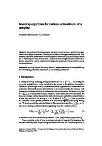
conventional detector jointly optimum

Probability of error for user 1

5. REFERENCES [1] S. Benedetto and E. Biglieri, Principles of Digital Transmission with Wireless Applications, NewYork: Kluwer/Plenum, 1999.

[3] R. Matzner, “An SNR estimation algorithm for complex baseband signals using higher order statistics,” Facta Universitatis, Series: Electronics and Energetics, Vol. 6, No. 1, pp. 41–52, 1993.

individually optimum σ2 individually optimum σ2 e

0.086

In this paper we have studied the behavior of the individually optimum receiver when it has partial knowledge of the noise variance. We have shown that the error probability is piecewise monotonic. It follows that the error probability under noise variance mismatch is lower bounded by the one of individually optimum receiver under perfect variance knowledge (this is clear since this receiver achieves minimum error probability) and upper bounded by the maximum between the BER of the conventional detector and of the BER of the jointly optimum receiver. This shows that underestimation of the noise variance is less detrimental than overestimation.

[2] C. Berrou, A. Glavieux, P. Thitimajshima, “Near Shannon limit error-correcting and decoding: Turbo codes,” Proc. ICC, Geneva, pp. 1064-1070, May 1993.

2−user synchronous CDMA

0.087

4. CONCLUSION

0.085

0.084

[4] D.R. Pauluzzi and N.C. Beaulieu. “A comparison of SNR estimation techniques for the AWGN channel.” IEEE Transactions on Communications, Vol. 48, (10), pp. 1681–1691, Oct. 2000.

0.083

0.082

0.081

0.08 2

0 σ =.5 1

2

3

4

5

6

7

8

9

10

σ2e

Fig. 2. Effect of noise variance mismatch mismatch on the individually optimum receiver Figure 2 illustrates proposition 2 and its corollary for the 2-user case. As it is analytically proven above, the error probability of the individually optimum receiver is a piecewise monotonic function of the estimated noise variance. In the case of positive signal to noise ratio for user 1 (A1 > σ 2 ), the BER of the conventional detector is greater than the BER of the jointly optimum receiver, which is known to be close to the BER of the individually optimum receiver [1, page 814]. This justifies a well known result in the community that underestimation of the noise variance is less detrimental than overestimation.

[5] H. Shin and J. H. Lee, “A channel reliability estimation for turbo decoding in rayleigh fading channels with imperfect channel estimates,” IEEE Communications Letters, pp. 503- 505, Nov. 2002. [6] T.A. Summers and S.G. Wilson, “SNR mismatch and online estimation in turbo decoding,” IEEE Transactions on Communications, Vol. 46, (4), pp. 421-423, April. 1998. [7] S. Verd´u, “Minimum Probability of error for asynchronous Gaussian multiple-access channels,” IEEE Trans. on Inf. Th., Vol. 32, pp. 85-96, Jan. 1986. [8] S. Verd´u, Multiuser detection, Cambridge Univ. Press, 1998. [9] A. Worm, P. Hoeher and N. Wehn. “Turbo-decoding without SNR estimation,” IEEE Communications Letters, pp. 193-195, June 2000.