snr and noise variance estimation in polarimetric sar data - Core

SNR AND NOISE VARIANCE ESTIMATION IN POLARIMETRIC SAR DATA Michelangelo Villano(1), Konstantinos P. Papathanassiou(1) (1)

German Aerospace Center (DLR), Microwaves and Radar Institute, Oberpfaffenhofen, 82234 Wessling, Germany. Email: [email protected]

ABSTRACT The problem of estimating the signal-to-noise ratio (SNR) of the cross-polarised channels and the noise variance in polarimetric synthetic aperture radar (SAR) data is dealt with. The Cramér-Rao Lower Bound (CRLB) is evaluated for the joint estimation of SNR of the cross-polarised channels and the noise variance, as well as for the SNR of the cross-polarised channels, in case the noise variance is known. Maximum likelihood (ML) estimators are then derived, one which jointly estimates the SNR of the cross-polarised channels and the noise variance and another which estimates the SNR of the cross-polarised channels, in case the variance is known. The performance of the estimators is assessed and a comparison with a coherence-based (CB) SNR estimator and an eigenvalue-based (EB) noise variance estimator is carried out. As far as the SNR estimation is concerned, both the ML and the CB estimator are positively biased, but the bias of the ML estimator is smaller than the bias of the CB estimator. As far as the noise variance estimation is concerned, the ML estimator is unbiased and efficient, while the EB estimator is negatively biased. The difference in the biases is also shown using TerraSAR-X fullypolarimetric data, acquired during the Dual Receive Antenna (DRA) campaign. 1.

(a)

INTRODUCTION

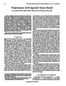
Fully polarimetric synthetic aperture radar (SAR) systems allow the extraction of physical information from the observed scattering of microwaves by surface and volume structures [1]. Fig. 1 shows the Pauli color-coded image and the coherence between the two cross-polarised channels, HV and VH, for a fully polarimetric data set, acquired by the German satellite TerraSAR-X over Lower Bavaria, Germany, during the Dual-Receive Antenna (DRA) campaign. As apparent, the coherence is quite low, not only over the two rivers, but also over some of the surrounding agricultural fields. For a monostatic system, where the transmitting and receiving antennas are placed at the same location, the data of the two cross-polarised channels are equal, but for the thermal noise, which adds in the receiver. A low coherence between the two cross-polarised channels, therefore, means that thermal noise is significant.

(b) Figure 1. TerraSAR-X fully polarimetric data set acquired over Lower Bavaria, Germany. (a)Pauli colorcoded image. (b) Coherence between the two crosspolarised channels (HV and VH).

The effect of thermal noise on polarimetric SAR data has been first analysed in [2], where it is examined how polarimetric measurements, such as the covariance matrix and the Stokes matrix, are affected by thermal noise and it is also pointed out as a first order correction can be applied to averaged covariance matrix or Stokes matrix values, if the noise variance is known. If such first order noise corrections are not applied, several measures commonly derived from polarimetric SAR data may give erroneous results, hence the importance of an unbiased and accurate estimate of the noise variance. Furthermore, an estimate of the signal-to-noise ratio (SNR) of the different polarimetric channels is also of importance, as different applications have different requirements in terms of SNR and the estimated SNR let us understand whether or not a data set is suitable for a given application. In particular, due to the low backscatter, the SNR of the cross-polarised channels can be critical, even considering the 3 dB gain resulting from symmetrisation [2].

SNR 

A2

(2)

2

We would like to estimate SNR and the noise variance σ2 from u1[i], i = 0..N-1, and u2[i], i = 0..N-1, under the stated assumptions. 3.

CRAMÉR-RAO LOWER BOUND

The Cramér-Rao lower bound (CRLB) is the minimum variance achievable by any unbiased estimator [3]. Therefore, if an estimator is unbiased and its variance is equal to the CRLB, it is the minimum variance unbiased (MVU) estimator [3]. The CRLB can be obtained from the natural logarithm of joint probability density function (PDF) of the 2N observables, which can be collected in an observation vector x x  u1 0 u1 1  u1 N  1 u2 0 u2 1  u2 N  1

T

(3)

Under the stated assumptions, the PDF of x is given by 2.

STATEMENT OF THE PROBLEM

Let us assume that calibrated single-look complex data, corresponding to the two cross-polarised channels of a polarimetric SAR system, are available and let us consider a set of N independent resolution cells, over which a distributed target extends. Let u1[i], i = 0..N-1, and u2[i], i = 0..N-1, be the complex amplitudes corresponding to the above mentioned N resolution cells for the two channels. As mentioned, the signals received by the two channels are equal, but for an additive term due to the thermal noise. Therefore, each of the two sequences uk[i], k =1, 2, can be written as the sum of a common sequence s[i], representing the useful signal, and a sequence wk[i], k =1, 2, representing the additive thermal noise u1 i   si   w1 i , i  0..N  1

u2 i   si   w2 i , i  0..N  1

px x  





1 exp  x H Cx 1x 2 N det(Cx )

(4)

where Cx is the 2N  2N covariance matrix of x. The elements of Cx are given by





C x i ,i  E si   w1 floori / N  i si   w1 floori / N  i   *

 A     SNR  1, i  0..2 N  1 2

2

2





C x i ,i  N  E si   w1 i si   w2 i   *

 A   SNR, i  0..N  1 2

(5)

2





C x i  N ,i  E si   w2 i si   w1 i   *

 A   SNR, i  0..N  1 C x i  N ,i  0, for all the other elements of the matrix 2

2

(1)

It is assumed that s[i], i = 0..N-1, are N independent realisations of a circularly symmetric Gaussian random variable with mean zero and variance A2. This is, in fact, the behaviour of a distributed scatterer, whose radar cross section (RCS) is equal to A2, in case the speckle is fully developed. It is also assumed that wk[i], k =1, 2, i = 0..N-1, are 2N independent realisations of a circularly symmetric Gaussian random variable with mean zero and variance σ2. Moreover, it is assumed that and s[i], i = 0..N-1, and wk[j], k =1, 2, j = 0..N-1, are uncorrelated. As s[i], i = 0..N-1, and wk[j], k =1, 2, j = 0..N-1 are two uncorrelated circularly symmetric Gaussian random variables, they are also statistically independent. The signal-to-noise ratio of the cross-polarised channels SNR is defined as

The covariance matrix Cx can be therefore rewritten as a block matrix  2 SNR  1I N  2 SNR I N  Cx    2 2  SNR  1I N    SNR I N

(6)

where IN is the identity matrix of size N. Recalling that the determinant and the inverse of a square block matrix M, written as in A B  M   C D

(7)

are given by [4] det M  det AD  BC

(8)

and [5]  A  BD1C M 1   1 1 1  D CA  BD C

 A 1BD  CA1B  D  CA1B1

1

1

The CRLB for the joint estimation of SNR and σ2 are therefore given by

  

(9)

respectively, the determinant and the inverse of the covariance matrix Cx are given by N

(10)

 

var ˆ 2 

and  SNR  1 1  2SNR  1 I N C  2   SNR I N  2SNR  1 1 x

SNR  IN 2SNR  1   SNR  1 IN  2SNR  1 



(11)

2 N 12 N 1

 x C i 0 j 0

2 N 1

* i

1 i, j

xj 



N 1

(12)



 C 1i,i xi   C 1i,i  N xi* xi  N  xi* N xi  2

i 0

(16)

2N

i 0

1  SNR  1 2 N 1 2 SNR N 1  xi    2 Re xi* xi  N  2    2SNR  1 i  0 2SNR  1 i  0





 

 1  SNR  1 SNR N 1 2  2 xi    2 Re xi* xi N    2SNR  1 i0 2SNR  1 i0 2 N 1





(17)

N

respectively. 3.2. Case of Known Noise Variance

   2 ln p x x    4N J SNR    E     2 2   SNR   2 SNR  1     

(18)

It therefore holds

 

and the natural logarithm of the PDF of Eq. 4 is therefore given by ln  px x   2 N ln    2 N ln  2  N ln 2SNR  1

4

In case the noise variance σ2 is known (e.g. physical measurements are available or a very accurate estimate has been carried out using the whole data set and assuming spatial stationarity), it is of interest to derive the CRLB for the SNR estimation. This is given by the inverse (or reciprocal) of the singleelement Fischer information matrix J(SNR)

respectively. The quantity xHCx-1x in Eq. 4 can be expanded as x H Cx 1x 

2SNR  12

and

det Cx    4 N 2SNR  1



 

var SNˆ R 

(13)

var SNˆ R 

2SNR  12

By comparison with Eq. 16, it can be noticed that the CRLB is by a factor of 2 better, if the noise variance σ2 is known.

3.1. Joint Estimation of SNR and Noise Variance

4.

The CRLB for the joint estimation of SNR and σ2 are given by the diagonal elements of the inverse of the 2  2 Fischer information matrix J(SNR, σ2) [3]

4.1. Joint Estimation of SNR and Noise Variance



J SNR,  2



   2 ln  px x    2 ln  px x    E  E  2 2   SNR   SNR    2 2    ln  p x    ln  px x  x  E    E  2 2    2      SNR 

 

 

(14)

 

4N 2N    2 SNR  12  2 2 SNR  1    2N 2N   2 4   2 SNR  1 

In particular, the inverse matrix J-1(SNR, σ2) is given by



J 1 SNR, 2



 2SNR  12  2 2SNR  1    2N 2N   2 4    2SNR  1    2N N

(15)

(19)

4N

MAXIMUM LIKELIHOOD ESTIMATION

The maximum likelihood (ML) estimates of SNR and σ2 are the values of SNR and σ2 for which the PDF of the observation vector in Eq. 4 is maximum [3]. In order to derive a closed-form expression for these estimates, the expression in Eq. 4 has to be maximised with respect to each of the two variables. As the logarithm is a strictly monotonic function, this is equivalent to maximise the logarithm of the PDF in Eq. 4, which is given in Eq. 13. In particular, the first-order partial derivatives (with respect to SNR and σ2) of the expression in Eq. 13 have to be set equal to zero   ln  px x  0  SNR   ln  p x  x  0 2   

 

(20)

By solving for SNR and σ2, one obtains the maximum likelihood SNR and noise variance estimates, which are given by



N 1

SNˆ RML 



2 Re u1* i u2 i  i 0 N 1

 u i  u i i 0

1

(21)

2

2

and

(a) N 1

2 ˆ ML 

 u i  u i i 0

1

2

2

(22)

2N

respectively. Figs. 2 and 3 display the relative bias and accuracy for the ML joint SNR and noise variance estimator for different values of N. As apparent, the ML noise variance estimator is unbiased and efficient, while the ML SNR estimator is positively biased.

(b) Figure 3. Performance plots for the ML SNR estimator for different values of N. (a) Relative bias. (b) Relative accuracy. 4.2. Case of Known Noise Variance In case the noise variance σ2 is known, the ML estimate of the SNR of the cross-polarised channels is obtained by setting to zero the first-order partial derivative with respect to SNR of the expression in Eq. 13

(a)

 ln px x  0 SNR

(23)

The ML estimate of SNR, which is also function of the noise variance σ2, is therefore given by N 1

SNˆ RML 

(b) Figure 2. Performance plots for the ML noise variance estimator for different values of N. (a) Relative bias. (b) Relative accuracy. The dashed lines represent the CRLB.

2



 u i  u i i 0

1

4 N 2

2

2



1 2

(24)

Fig. 4 displays the relative bias and accuracy for the ML SNR estimator, in case the variance is known, for different values of N. In this case, the ML SNR estimator is unbiased and efficient.

(a)

(a)

(b)

(b)

Figure 4. Performance plots for the ML SNR estimator in case of known variance for different values of N. (a) Relative bias. (b) Relative accuracy. The dashed lines represent the CRLB.

Figure 5. Performance plots for the ML noise variance estimator for different values of N. (a) Relative bias. (b) Relative accuracy.

5.

COMPARISON WITH OTHER ESTIMATORS

The ML estimators can be compared to other estimators in terms of relative bias and accuracy. 5.1. Noise Variance Estimation Concerning the noise variance estimation, a noise variance estimator has been proposed in [6], which estimates the noise variance as the minimum of the two eigenvalues of the covariance matrix of the 2dimensional vector containing the data of the two crosspolarised channels

 

 E u1u1* covu1 u2    *  E u1 u2

 Eu u   Eu u  * 1 2 * 2 2

The bias can be also observed on real data. Fig. 6 shows the histograms of estimated noise variances, obtained applying the ML and the EB estimators to a 1024  1024 pixel patch extracted from a fully polarimetric data set, acquired by the German satellite TerraSAR-X over Austfonna, Svalbard, Norway, during the dual receive antenna (DRA) campaign. An 11  11 pixel window has been used.

(25)

The expression of the noise variance estimate, from now on referred to as eigenvalue-based (EB), is given by [7] 2 ˆ EB 

1 2N

N 1

 u [i] i 0

1

2



1 2N

N 1

 u [i] i 0

2

2

2

(26)



N 1 1  1 N 1 1 N 1  N 1 2 2 2  2   u1 [i ]   u 2 [i ]     u1 [i ]   u 2 [i ]   N  2 i 0 2 i 0   i 0  i 0 

N 1

 u [i]u [i] i 0

* 1

Figure 6. Histograms of the ML and EB noise variance estimates for a patch of TerraSAR-X fully polarimetric data, acquired over Austfonna, Svalbard, Norway.

2

2

Fig. 5 displays the relative bias and accuracy for the EB noise variance estimator for different values of N. As apparent, the EB noise variance estimator is negatively biased. As the ML noise variance estimator is unbiased, the ML estimator should be preferred to the EB estimator.

A similar estimator is reported in [6], where the noise variance is estimated as the smallest eigenvalue of the 4  4 coherency matrix. 5.2. SNR Estimation Concerning the estimation of the SNR of the crosspolarised channels, it can be estimated from the

coherence magnitude between the two cross-polarised channels, defined as [8] N 1

ˆ 

 u [i]u [i] k 0

* 2

1

N 1

N 1

 u [i]  u [i] k 0

2

1

i 0

(27) 2

Even in this case the difference of biases can be observed on real data. Fig. 8 shows the histograms of estimated SNR, obtained applying the ML and the CB estimators to the 1024  1024 pixel patch extracted from the Austfonna data set. An 11  11 pixel window has been used.

2

The SNR influences the coherence magnitude according to the following formula [8]



1

(28)

1 1 SNR

which can be inverted to obtain a SNR estimate, from now on referred to as coherence-based (CB) SNR estimate

SNˆ RCB 

ˆ

(29)

1  ˆ

Fig. 7 displays the relative bias and accuracy for the CB SNR estimator for different values of N. As apparent, the CB SNR estimator is positively biased . Comparing Figs. 3 and 7, it can be noticed that the bias of the CB SNR estimator is larger than the bias of the ML estimator by a factor of two for high SNR values and even more for low SNR values.

Figure 8. Histograms of the ML and CB SNR estimates for a patch of TerraSAR-X fully polarimetric data, acquired over Austfonna, Svalbard, Norway. 6.

The problem of estimating the SNR of the crosspolarised channels and the noise variance has been dealt with. The CRLB has been derived and ML estimators are proposed, which perform better than other estimators in terms of relative bias and accuracy. REFERENCES 1.

2.

3.

4. (a)

5. 6.

7.

(b) Figure 7. Performance plots for the ML SNR estimator for different values of N. (a) Relative bias. (b) Relative accuracy.

CONCLUSION

8.

Lee J.S. & Pottier E. (2009). Polarimetric Radar Imaging. From Basics to Applications, CRC Press, New York. Freeman A. (1993), “The Effect of Noise on Polarimetric SAR Data”, Proc. IGARSS, Tokio, Japan, pp.799–802. Kay S.M. (1993). Fundamentals of Statistical Signal Processing: Estimation Theory, PrenticeHall, Upper Saddle River, NJ. Silvester J. R. (2000). “Determinants of block matrices”, Mathematical Gazette, 84(501), pp. 460– 467. Ayres, F. Jr. (1962). Matrices, Shaum's Outline Series, McGraw-Hill, New York. Hajnsek I., Papathanassiou K.P. & Cloude S.R. (2001), “Removal of Additive Noise in Polarimetric Eigenvalue Processing”, Proc. IGARSS, Sidney, Australia, pp.2778–2780. Cloude, S.R. (2011). Introduction to Pol-InSAR, in Materials of the “Advanced Course on Radar Polarimetry”, 17-21 January 2011, ESA-ESRIN, Frascati, Rome, Italy (http://earth.eo.esa.int/pub/polsarpro_ftp/RadarPol_ Course11/Wednesday19/BasicsPoinsar_theory_Cloude.pdf). Bamler R. & Hartl P. (1998), “Synthetic aperture radar interferometry”, Inv. Probl., 14, pp. R1-R54.