Mar 21, 2011 - csz = a. â. 2ϵ. â cs. ,. (2.15) where â¡ d/dy. It is useful to list the ...... value for λ/Σ as discussed in section 3.3, since P,XXX is not constrained.
arXiv:1102.0275v2 [astro-ph.CO] 21 Mar 2011
Non-Gaussianity in single field models without slow-roll Johannes Noller and Jo˜ao Magueijo Theoretical Physics, Blackett Laboratory, Imperial College, London, SW7 2BZ, UK
Abstract We investigate non-Gaussianity in general single field models without assuming slow-roll conditions or the exact scale-invariance of the scalar power spectrum. The models considered include general single field inflation (e.g. DBI and canonical inflation) as well as bimetric models. We compute the full non-Gaussian amplitude A, its size fNL , its shape, and the running with scale nN G . In doing so we show that observational constraints allow significant violations of slow roll conditions and we derive explicit bounds on slow-roll parameters for fast-roll single field scenarios. A variety of new observational signatures is found for models respecting these bounds. We also explicitly construct concrete model implementations giving rise to this new phenomenology.
Contents 1 Introduction
1
2 Single field models without slow-roll 2.1 Observational constraints on (non)-slow-roll . . . . . . . . . . . . . . . . . . 2.2 The spectral index ns . . . . . . . . . . . . . . . . . . . . . . . . . . . . . . . 2.3 The tensor-to-scalar ratio r . . . . . . . . . . . . . . . . . . . . . . . . . . .
3 4 6 7
3 Non-Gaussianity 3.1 The full amplitudes 3.2 fN L . . . . . . . . . 3.3 Shapes . . . . . . . 3.4 The running nN G .
. . . .
9 10 12 15 20
4 Concrete model examples 4.1 Fast-roll DBI inflation . . . . . . . . . . . . . . . . . . . . . . . . . . . . . . 4.2 Fast-roll inflation with Σλ � 1 . . . . . . . . . . . . . . . . . . . . . . . . . 4.3 Bimetric theories . . . . . . . . . . . . . . . . . . . . . . . . . . . . . . . . .
23 24 25 26
5 Conclusions
27
A Appendix A.1 Details on the computation of the three-point function . . . . . . . . . . . . A.2 General expressions for fNL and nN G . . . . . . . . . . . . . . . . . . . . . .
29 29 31
1
. . . .
. . . .
. . . .
. . . .
. . . .
. . . .
. . . .
. . . .
. . . .
. . . .
. . . .
. . . .
. . . .
. . . .
. . . .
. . . .
. . . .
. . . .
. . . .
. . . .
. . . .
. . . .
. . . .
. . . .
. . . .
. . . .
. . . .
. . . .
. . . .
. . . .
. . . .
Introduction
Non-Gaussianity as probed by upcoming experiments such as Planck will be a very powerful tool for selecting models of primordial structure formation [1, 2, 3, 4, 5, 6]. One of the most interesting questions one may hope to answer is: Are single field models of structure formation sufficient, or do we need multiple fields to meet observational constraints? The hallmark of single field models that generate large non-Gaussianity is often thought to be an equilateral type non-Gaussian shape [7, 8, 9, 10, 11, 12]. Known modifications to this shape can be achieved by introducing, for example, non-Bunch-Davies vacua [7, 13, 14, 15, 16] or resonant running [10, 17, 18, 19, 20]. However, models with additional fields, such as multifield inflation [21, 22, 23, 24, 25, 26, 27, 28, 29, 30, 31, 32, 33, 34, 35] or models adding curvaton fields [36, 37, 38, 39, 40, 41, 42, 43, 44], can give rise to a much greater variety of non-Gaussian signatures (see e.g. [33]). It is therefore interesting to investigate whether multifield models are really unique in predicting all such alternative shapes. 1
In this paper we demonstrate that non-slow-roll single field models can produce a much richer variety of detectable non-Gaussian signatures than those following from slow-roll conditions. Typically slow-roll conditions are expected to be imposed by observational constraints derived from primordial structure formation [1] and from bounds arising by requiring solutions of e.g. flatness, homogeneity and isotropy problems. In [8] it was shown that for exactly scale-invariant non-canonical models, a much wider range of slow-roll parameters is allowed than those satisfying slow-roll conditions, whilst still satisfying all observational bounds. We extend this work by dropping the requirement of exact scale-invariance, explicitly computing the corresponding new bounds for slow-roll parameters and showing that an even wider range of parameters becomes observationally viable. Non-Gaussianities for non-slow-roll single field models have been previously computed for the case of exact scale invariance ns = 1 [8] and that of an effective DBI type action [11]. We will generalize this work, restricting ourselves to expanding solutions as provided, for example, by inflationary [45] and bimetric models [46, 11]. Contracting models have been considered in the context of ekpyrotic/cyclic models [47, 48] and effective perfect fluid models [49, 50]. 1 In this paper we hope to complete the picture in the expanding case by deriving non-Gaussianities for general single field models without assuming smallness of slow-roll parameters �i or exact scale invariance (ns = 1). We investigate the phenomenology associated with such models, showing that they have several distinct observable signatures. These include a generically large running of non-Gaussianity nN G with scale, the suppression of the size of non-Gaussianity fNL by non-slow-roll �i and the emergence of qualitatively new shapes for single field models e.g. ones with dominant contributions in the folded limit 2k1 = 2k2 = k3 . These considerations widen the number of potential future observations that could be explained by single field models. And even if future measurements turn out to favor multifield models, it is still important to fully understand the potential effects of individual fields that may participate in such models. The plan of the paper is as follows. In section 2 we set the stage by considering the twopoint correlation functions for scalar and tensor perturbations in general single field models. We compute the resulting observational constraints on slow-roll parameters and also summarize bounds coming from other sources. Then, in section 3, we compute non-Gaussianities, explicitly giving the full amplitudes for general single field models without assuming slow-roll conditions or exact scale-invariance (section 3.1). Observational signatures are considered in detail for fNL (section 3.2), non-Gaussianity shapes (section 3.3) and running with scale nN G (section 3.4). In section 4 concrete models are provided for the phenomenologically interesting cases by explicitly constructing their actions. In section 5 we conclude, summarize results and point out intriguing possibilities for further work.
1
While this paper was being finished, references [51, 52] appeared, which further investigate contracting models. [52] also considers strong coupling constraints for expanding models.
2
2
Single field models without slow-roll
The models we shall consider have an action of the form [53, 54] � � Z √ R 4 + P (X, φ) , S = d x −g 2
(2.1)
where the pressure P is a general function of a single scalar field φ and its kinetic term X = − 12 g µν ∂µ φ∂ν φ. For a canonical field P (X, φ) = X − V (φ). In principle P can contain higher derivatives of the field φ as well, however such terms are expected to be suppressed by the UV cut-off scale in an effective field theory. This motivates studying an action of the form (2.1), which is the most general Lorentz invariant action for a single scalar field minimally coupled to gravity that contains at most first derivatives of the field. The pressure p and energy density ρ for these models are given by p = P (X, φ) , ρ = 2XP,X − P (X, φ) ,
(2.2)
where P,X ≡ ∂P/∂X. We will find it useful to characterize the non-canonical nature of (2.1) with the following quantities [55] P,X P,X = , ρ,X P,X + 2XP,XX H 2� 2 Σ = XP,X + 2X P,XX = 2 , cs 2 λ = X 2 P,XX + X 3 P,XXX , 3
c2s =
(2.3) (2.4) (2.5)
where cs is the adiabatic speed of sound. An infinite hierarchy of slow-roll parameters � and �s and their derivatives can then be constructed for a theory (2.1) with an FRW metric with scale factor a(t) and corresponding Hubble rate H(t) = a/a. ˙ These hierarchies are �≡−
H˙ �˙ , η≡ , ... 2 H �H
�s ≡
;
c˙s �˙s , ηs ≡ , ... cs H �s H
(2.6)
The slow-roll approximation requires that �, η...�s , ηs ... � 1 and accelerated expansion takes place when � < 1. Note that these definitions are more general than alternative definitions in terms of the scalar potential and its derivatives, which assume canonical kinetic terms. Perhaps more fittingly (2.6) have therefore also been dubbed “slow-variation parameters” [56, 57, 58]. DBI inflation [59], for example, is slow varying in this sense yet allows steep potentials and hence the inflaton is not slow-rolling. However, in order to agree with convention and avoid confusion, we will refer to (2.6) as slow-roll parameters from now on. Truncating slow-roll parameters at some derivative order, setting the remainder to zero, allows us to approximate H and cs with Taylor expansions. Following [8, 11] we consider 3
models where slow-roll conditions are broken by �, �s ∼ O(1). We will assume that �, �s are approximately constant, so that slow-roll conditions still hold for the remaining negligible parameters η, ηs ... ≈ 0.
2.1
Observational constraints on (non)-slow-roll
Large classes of both inflationary and bimetric models can be described by action (2.1). Bimetric models generically have � > 1 and are discussed in detail in section 4.3. For the inflationary branch � < 1, however, observations can be used to constrain the allowed values of slow-roll parameters �, �s . These constraints are derived throughout the paper and we summarize the resulting bounds upfront here. The observational bounds considered are the following: • The spectral index ns : The spectral index of scalar perturbations ns is computed in section 2.2. In terms of the slow-roll parameters it can be written as ns − 1 =
2� + �s . �s + � − 1
(2.7)
The WMAP bounds on ns in the presence of tensor perturbations are ns = 0.973±0.028 at 2σ. Note that these constraints are dependent on e.g. the precise value of H0 [1] and the physics of reionization [60]. Contrary to the canonical field case, for a general single field model (2.1) the smallness of ns − 1 � 1 no longer automatically translates into a constraint on � alone. Instead, for any parameter �, one can find a corresponding speed of sound profile parameterized by �s , which returns any desired spectral index. Bounds on ns therefore only translate into constraints on the relation between � and �s , not on either variable by itself. • The tensor-to-scalar ratio r: The tensor-to-scalar ratio r is similarly constrained by CMB observations. The WMAP experiment provides a bound r < 0.24 at 2σ [1]. In section 2.3 we discuss how the first order relation r = 16�cs is modified in general single field models without slow-roll and compute corresponding bounds on slow-roll parameter �. We find � . 0.4. (2.8) • The running nN G : Introducing non-canonical kinetic terms can lead to a strong running of non-Gaussianities with scale nN G [8, 61, 62, 63], irrespective of whether the 2-point correlation function as measured by ns is near-scale-invariant or not. This can impose further constraints on �. If non-Gaussianities show a blue tilt, this means they peak on smaller scales. For a perturbative treatment to be applicable, one therefore needs to ensure that non-Gaussianities on the smallest observable scales are not too large for a perturbative approach to break down. In section 3.4 we identify under which conditions non-Gaussianities are blue tilted and what constraints on � follow. 4
We show that constraints are in principle model-dependent. However, for a very large subclass of models one can obtain rough bounds � . 0.3
if
fNL (CMB) ∼ O(100)
� . 0.5
if
fNL (CMB) ∼ O(1).
(2.9) (2.10)
This result agrees with bounds obtained in the exactly scale invariant case [8]. However, we show that these limits are in fact relatively insensitive to the precise value taken by ns , but strongly depend on parameters cs , Σ, λ. • The Big Bang problems: Observational bounds only place constraints on primordial perturbations for a small range of scales: CMB (∼ 103 Mpc) to galactic scales (∼ 1Mpc). ns ,r and nN G as discussed above are therefore only observationally constrained over these scales. In an inflationary setup this corresponds to approximately 10 e-folds, where the number of e-folds N of inflation is given by dN = −Hdt. In order to resolve the flatness, homogeneity and isotropy problems of cosmology, a greater number of e-folds is needed. Conventionally this is chosen N ∼ 60, although the minimal amount of e-folds needed is not very well defined and depends e.g. on the energy scale of inflation, details of the reheating mechanism, etc. [64] The inflationary condition � < 1 is sufficient to yield an attractor solution towards flatness, homogeneity and isotropy [8]. A large number of e-folds requires � < 1 for several Hubble times, which is controlled by parameter η. As we consider cases for which η ∼ 0 � 1, the fractional change in � per Hubble time is small and hence starting with � < 1 guarantees that a prolonged phase of inflation takes place. However, we should note that several other solutions are possible as well. For example, the scaling phase responsible for near-scale-invariant perturbations on observable scales may be followed by a different inflationary phase (scaling or not) [8]. Particle physics may suggest that inflation is actually a multiple step process, where one relatively short initial phase is responsible for observable structure on very large scales [65]. Inflation then ends and is followed by (an)other phase(s) of accelerated expansion later. It could also be that an altogether different mechanism2 resolves the problems in question here [66, 67, 68]. In any case no competitive constraints on � can be derived from consideration of these cosmological problems. Also note that bimetric models resolve these problems in a radically different way [66, 67, 68]. Inflationary models of the type envisaged by (2.1), with � . 0.3, meet all the observational bounds. 2
And of course, as the flatness, homogeneity and isotropy problems are essentially initial value problems, the correct initial values may be set by pre-inflationary physics. Whilst such a solution may be very nondefinitive and as such less appealing, one should keep in mind that there is certainly no guarantee that all cosmological puzzles can be answered at energy scales we have (in-)direct access to.
5
2.2
The spectral index ns
In this section we sketch the calculation of the primordial power spectrum of scalar perturbations. Scalar perturbations in the metric ds2 = (1 + 2Φ)dt2 − (1 − 2Φ)a2 (t)γij dxi dxj ,
(2.11)
can be analyzed in terms of the the gauge invariant curvature perturbation ζ ζ=
2ρ 5ρ + 3p Φ˙ Φ+ , 3(ρ + p) 3(ρ + p) H
(2.12)
where p and ρ are the background pressure and energy density respectively. Perturbing (2.1) to quadratic order in ζ one obtains [54] "� � # 2 2 Z MPl dζ ~ 2 , S2 = d3 xdτ z 2 − c2s (∇ζ) (2.13) 2 dτ √ where τ is conformal time, and z is defined as z = a 2�/cs . As a consequence of considering non-canonical kinetic terms, we have introduced a dynamically varying speed of sound. This means it is convenient to work in terms of the “sound-horizon” time dy = cs dτ instead of τ [8]. For the case relevant here, i.e. η = ηs = 0, one finds cs . (2.14) y= (� + �s − 1)aH In terms of y-time the quadratic action takes on the familiar form √ h i 2 Z √ MPl a 2� 3 2 02 2 ~ S2 = d xdy q ζ − (∇ζ) , q ≡ cs z = √ , 2 cs
(2.15)
where 0 ≡ d/dy. It is useful to list the behavior in proper time τ and in y-time of some relevant quantities for later reference: 1
a ∼ (−τ ) �−1 1
a ∼ (−y) �s +�−1
; ;
�s
cs ∼ (−τ ) �−1 �s
cs ∼ (−y) �s +�−1
−�
;
H ∼ (−τ ) �−1 ,
;
H ∼ (−y) �s +�−1 .
−�
(2.16)
Upon quantization the perturbations are expressed through creation and annihilation operators as follows, ζ(y, k) = uk (y)a(k) + u∗k (y)a† (−k)
[a(k), a† (k0 )] = (2π)3 δ 3 (k − k0 ).
,
(2.17)
In terms of the canonically-normalized scalar variable v = MPl qζ the equations of motion for the Fourier modes are � � q 00 2 00 vk + k − vk = 0 . (2.18) q 6
If �, η, �s , ηs are constant, as is the case here, one can solve for q 00 /q exactly [69]: � � q 00 1 1 2 = 2 ν − . q y 4
(2.19)
The precise solution for vk (y) depends on which initial vacuum is chosen. Typically this is the Bunch-Davis vacuum, which is defined to be the state annihilated by a(k) as t → −∞. With this vacuum choice the solution for vk (y) is √ π√ vk (y) = −y Hν(1) (−ky). (2.20) 2 (1)
where Hν are Hankel functions of the first kind. However, we note that different adiabatic vacuum choices are possible in principle and also have distinctive observational signatures (particularly non-Gaussianities) [9, 14, 15, 7]. For the modes defined in (2.17) one finds r 1/2 1/2 cs π√ cs √ vk (y) = −yHν(1) (−ky). (2.21) uk (y) = 3/2 aMPl 2 � aMPl 2� Therefore the 2-point correlation function for ζ is: hζ(k1 )ζ(k2 )i = (2π)5 δ 3 (k1 + k2 )
Pζ , 2k13
(2.22)
where the expression for the power spectrum Pζ is Pζ ≡
¯2 1 3 (�s + � − 1)2 22ν−3 H 2 k |ζ | = . k 2 2π 2 2(2π)2 � c¯s MPl
(2.23)
Note that we have approximated the propagator uk (y) assuming ns − 1 � 1 in accordance with observations here (for details see appendix A.1 - a more general expression for Pζ can be found in [69]). The bar symbol means that the corresponding quantity has to be evaluated, for each mode k, at sound horizon exit, i.e. when y = k −1 . The spectral index ns is finally given by dlnPζ 2� + �s ns − 1 ≡ = 3 − 2ν = . (2.24) dlnk �s + � − 1 Therefore exact scale invariance obtains when ns = 1, i.e. �s = −2�. Constraints on ns consequently translate into relational constraints on � and �s . Importantly this means no direct bound on either � or �s can be obtained in this way, because for any parameter choice � one can find an appropriate �s to yield a (near)scale-invariant solution. This is in contrast to the case of canonical fields, where the smallness of ns − 1 requires � to be small.
2.3
The tensor-to-scalar ratio r
In inflation [45] primordial quantum tensor fluctuations are sourced on sub-horizon scales before leaving the horizon and freezing out in analogy to scalar fluctuations. Present observational upper bounds on the tensor-to-scalar ratio r therefore constrain the amount of 7
gravity waves that could have been generated in the early universe. Here we use bounds on r to constrain slow-roll parameter �. Note that bimetric models of the primordial epoch do not resolve the horizon problem for gravitational waves [46]. As no quantum tensor fluctuations are amplified to become classical outside the horizon one does not expect any significant primordial gravitational wave contribution for these models. Such models therefore predict r ≈ 0. The action governing tensor modes is [69] 1 S= 2
Z
� � 00 � 2 Z � X a 0 2 2 2 |˜ vk,n | dη dk v˜k,n − k − a n=1 3
(2.25)
where the sum runs over the two distinct polarization modes and we have introduced v˜ to distinguish between variables v˜ and v associated with tensor and scalar perturbations Pl respectively. The action is written in terms of a Mukhanov-Sasaki variable v˜k,n = a(η)M hk,n , 2 where a is the scale factor of the FRW metric. Upon quantization v˜ can be expressed in terms of creation and annihilation operators as ˆ˜k,n + v˜k∗ (η)a ˆ˜† . vˆ˜k,n = v˜k (η)a k,n
(2.26)
The equation of motion for tensor modes can then be written as � 00 � a 00 2 v˜k + k − v˜k = 0. a
(2.27)
Accordingly we can now write down the power spectrum of tensor perturbations, where the sum again runs over polarization modes 2 k3 X h|hk,n |2 i, Ph = 2 2π n
(2.28)
which can be found to be [57, 69] √ 2 2 2µ−3 Γ(µ) 2µ−1 2H Ph = 2 Γ(3/2) (1 − �) πMpl
,
(2.29)
k=aH
where
1 1 + . (2.30) 1−� 2 Importantly the tensor power spectrum is evaluated at horizon crossing for the tensor modes. For general theories with a non-canonical kinetic term (2.1) this horizon is different from the corresponding horizon for scalar perturbations. The spectral index of tensor perturbations nt then is −2� nt = . (2.31) 1−� 8 µ=
The tensor-to-scalar ratio r is given by 2 � �2 2µ−1 Hh (1 − �) Γ(µ) 2µ−3 r≈2 3 � 16cs (kζ )� 2 (�s + � − 1) Γ 2 Hζ
(2.32)
where cs has to be evaluated at scalar horizon crossing and Hh and Hζ correspond to the Hubble factor at freeze-out for tensor and scalar modes respectively [57].3 Note that the dependence on the ratio of H at different horizon crossings can induce a strong scale dependence for r. Present-day observational constraints limit r . 0.3. The WMAP 95 % confidence level bound is r < 0.24 [1].4 For a given value of ns this can therefore be used to constrain �cs (kζ ). Ref [70] perform an MCMC sampling for general single field models (2.1) to find �cs < 0.023 at 2σ for a flat prior (note that the result is somewhat prior dependent). For a horizon crossing sound speed of c¯s = 0.1 this corresponds to � . 0.23 which agrees with the approximate bound derived by [8]. However, as we will show in the following section single field models with lower sound speeds c¯s ∼ 0.05 can satisfy current bounds on the size of non-Gaussianity, so that this bound on � can be relaxed to obtain � . 0.4
(2.33)
for general single field models as considered here (2.1).
3
Non-Gaussianity
In this section we compute the 3-point correlation function for the curvature perturbation ζ. Perturbing (2.1) to cubic order in ζ one obtains the effective action derived in [55, 7]. The result is valid outside of the slow-roll approximation and for any time-dependent sound speed: S3
(
� � ˙3 � � ζ 1 a3 � + 4 (� − 3 + 3c2s )ζ ζ˙ 2 = MP l dtd x −a Σ 1 − 2 + 2λ 3 cs H cs a� � ˙ + 2 (� − 2�s + 1 − c2s )ζ(∂ζ)2 − 2a 2 ζ(∂ζ)(∂χ) cs cs � � � 3 a�d η � � δL 2˙ 2 2 2 ζ ζ + + (∂ζ)(∂χ)∂ χ + (∂ ζ)(∂χ) + 2f (ζ) , 2c2s dt c2s 2a 4a δζ 1 2
Z
3
3
3
(3.1)
As a comparison with (2.23) shows, we have assumed ns −1 = 3−2ν � 1 here, i.e. near-scale-invariance. This bound is obtained assuming nt = −r 8 , however. The relation between nt and r is of course more involved for general single field models as a comparison between (2.31) and (2.32) shows. However, given that we obtain a red tilt of tensor modes (and Ph therefore peaks on the largest scales) the bound on r should only weakly depend on the precise value of the tilt. 4
9
where dots denote derivatives with respect to proper time t, ∂ is a spatial derivative, and χ is defined as a2 � ∂ 2 χ = 2 ζ˙ . (3.2) cs Note that the final term in the cubic action, 2f (ζ) δL | is proportional to the linearized δζ 1 equations of motion and can be absorbed by a field redefinition ζ → ζn + f (ζn ) - for details see appendix A.1. At first order in perturbation theory and in the interaction picture, the 3-point function is given by [71, 55, 7] Z t dt0 h[ζ(t, k1 )ζ(t, k2 )ζ(t, k3 ), Hint (t0 )]i , (3.3) hζ(t, k1 )ζ(t, k2 )ζ(t, k3 )i = −i t0
where Hint is the Hamiltonian evaluated at third order in the perturbations and follows from (3.1). Vacuum expectation values are evaluated with respect to the interacting vacuum |Ωi. The 3-point correlation function is conventionally expressed through the amplitude A hζ(k1 )ζ(k2 )ζ(k3 )i = (2π)7 δ 3 (k1 + k2 + k3 )Pζ2
1 A. Πj kj3
(3.4)
Also by convention the power spectrum Pζ in the above formula is calculated for the mode K = k1 +k2 +k3 . By using (2.17) we can now calculate the amplitudes for each term appearing in the action (3.1). Using a self-evident notation the overall amplitude is therefore given by A = Aζ˙3 + Aζ ζ˙2 + Aζ(∂ζ)2 + Aζ∂ζ∂χ + A�2 , ˙
(3.5)
where A�2 accounts for the ∂ζ∂χ∂ 2 χ and (∂ 2 ζ)(∂χ)2 terms in the action (3.1). In the following subsections we first present the main result (Sec. 3.1), which is a general expression for A where � is not constrained to satisfy � � 1 are given. We then study three physically interesting properties of these three-point functions: The size of the amplitude as parameterized by the variable fN L (Sec. 3.2), its shape (Sec. 3.3) and the running of the non-Gaussianity nN G (Sec. 3.4). Current observational bounds are also discussed for these properties.
3.1
The full amplitudes
We first present results for the full non-Gaussian amplitude A. Details of the calculation are given in appendix A.1. We stress that our results do not assume slow-roll conditions for �, �s and are therefore valid even when these parameters become �, �s ∼ O(1). Providing the full amplitudes here will hopefully prove useful for the computation of non-slow-roll nonGaussianities for specific single field models in the future. For the exactly scale-invariant case analogous non-slow-roll results were presented in [8] and for an effective DBI type action 10
these have been derived in [11] without assuming scale-invariance. However, as we will see in the following subsections, it is precisely the part of the amplitude that vanishes in DBI type models that is instrumental for much of the new phenomenology we find for general slow-roll violating single field models (2.1). The following variables will be useful in computing amplitudes α1 = ns − 1 = 3 − 2ν =
2� + �s �s + � − 1
;
α2 =
2� − �s �s + � − 1
Also note that we can write the parameter λ as [55, 8] � � Σ 2fX − 1 λ= −1 6 c2s where
(3.6)
(3.7)
X˙ ∂H ��s , �X = − 2 , (3.8) 3�X H ∂X and we note that there is in principle no dynamical requirement fixing �X (and hence fX ) to be small or large, even in the presence of constraints for � [55]. For DBI models (discussed in 4.1) fXDBI = 1 − c2s , so consequently the first term in the action (3.1) vanishes and there is no Aζ˙3 contribution to the amplitude. For the computation of Aζ˙3 we otherwise assume for simplicity that fX (and hence the kinetic part of �, �X ) is constant. Computing the amplitude in this way for each term in the action (3.1) we obtain �n −1 � � 1 k1 k2 k3 s � 2 Aζ˙3 = 2 (� + � − 1)(f − 1)I ¯ (� + � − 1)I ; 3 (α2 ) + c 3 (α1 ) ˙ ˙ s X s s ζ ζ 2¯ cs 2K 3 � �n −1 � 1 k1 k2 k3 s � 2 Aζ ζ˙2 = 2 (� − 3)I (α ) + 3¯ c I (α ) ; 2 2 ˙ ˙ 2 1 s ζζ ζζ 4¯ cs 2K 3 � �n −1 � k1 k2 k3 s � 1 (� − 2�s + 1)Iζ(∂ζ)2 (α2 ) − c¯2s Iζ(∂ζ)2 (α1 ) ; Aζ(∂ζ)2 = 2 3 8¯ cs 2K � �n −1 � k1 k2 k3 s � 1 −� I (α ) ; Aζ∂ζ∂χ = 2 ˙ ˙ 2 ζ∂ζ∂χ 4¯ cs 2K 3 � �n −1 � 1 k1 k2 k3 s � 2 A�2 = � I�2 (α2 ) , (3.9) 2 3 16¯ cs 2K fX =
where απ k12 k22 k32 Iζ˙3 (α) = cos Γ(3 + α) ; 2 K3 " # X X απ 1 1 Iζ ζ˙2 (α) = cos Γ(1 + α) (2 + α) ki2 kj2 − (1 + α) 2 ki2 kj3 ; 2 K i 5 is often quoted [77, 74], non-Gaussianity from models with lower fNL may be detected depending on the shape, if it has a significant amplitude in regions not probed by fNL . As a unique shape template is provided by models with cs � 1, deriving constraints for the full particular shape may be a promising strategy here and allow detection of low fNL signatures. 6 A complete basis capable of describing arbitrary shapes in k-space in principle has infinitely many “shape-members”. However, for the models considered here these three basis shapes will be sufficient.
14
Current WMAP limits on fNL for each of these shapes are [1] equil fNL = 26 ± 240 (95% CL), local fNL = 32 ± 42 (95% CL), orth = −202 ± 208 (95% CL). fNL
3.3
(3.17)
Shapes
In the previous section the information contained in A was condensed into a single parameter, fNL . However, there is vastly more information available, encoded in the functional dependence of A [75, 76, 77]. This is uniquely specified by the four parameters �, ns , c¯s , fX .7 In order to disentangle effects from a possible running of A with wavenumber K and the shapes themselves, in this section we present the shape of the amplitude at fixed K. In interpreting the shapes shown in this section it may be useful to emphasize that from (3.11) it follows that a good estimate for the size fNL corresponding to a given plotted shape (we normalize one wavevector k and hence plot A(1, k1 , k2 )/(k1 k2 )) is the value of the plotted amplitude in the equilateral limit. In the near future the shape and running of A will hopefully become experimentally accessible and, if a significant amount of non-Gaussianity is detected, will greatly constrain models of structure formation in the early universe. After all, at present these models are only observationally constrained to fit or respect upper limits on a number of single value parameters (The amplitude of scalar perturbations A, its spectral tilt nS , fNL , the tensorto-scalar ratio r). Fitting a full function would prove far more challenging and provide a strong model selection tool. The prototypical shape that has been associated with significant non-Gaussianity in single-field models is one of the equilateral type [7, 8, 9, 10, 11], where the amplitude peaks in the limit k1 = k2 = k3 . This is in contrast to e.g. multifield models which can also give rise to strong local contributions to A (i.e. peaking in the squeezed limit k1 ≈ k2 � k3 ) [9] via superhorizon interactions local in position space. This is because superhorizon evolution is local in space, as different regions are not causally connected with each other. Therefore any amount of non-Gaussianity generated after horizon exit is also local in position space and hence not local in k-space. It consequently peaks in the squeezed limit. In single field models, on the other hand, ζ is frozen in upon horizon exit, so no superhorizon evolution takes place. Far inside the horizon modes typically oscillate and their contributions to A average out. For known exceptions to this see [14, 15, 7, 10, 17, 18]. Thus A is almost completely sourced by modes exiting the horizon at similar times and hence with similar wavelengths. Consequently A peaks in the equilateral limit. An interesting question to ask is therefore: Considering deviations from slow-roll and 7
Note that there is an issue of choice here as we have six variables �, �s , ns , c¯s , fX , λ/Σ and two constraint equations (2.24) and (3.13). For instance specifying �, �s , c¯s , λ/Σ therefore also fixes the amplitude.
15
0.055 0.15
0.06 1.0
0.05
0.050
1.0
1.0 0.10
0.045
0.04
0.05
0.040
0.03 0.0
0.5
0.5
0.5
0.5
1.0
0.5
0.0
0.5
0.0
0.0
1.0
0.0
1.0
0.0
-10 0.06 1.0
0.05
0.4
-20
0.04
0.3 0.2
-40
0.03 0.0
0.5
1.0
1.0
-30
0.5
0.5
0.5
1.0
0.5
0.0
0.5
0.0
0.0
1.0
0.0
1.0
0.0
6
-1 0.06 1.0
0.05
-2
1.0
1.0
4
-3 0.04
2 -4
0.03 0.0
0.5
0.5
0.0
0.5
0.5
0.5
1.0
0.5
0.0
0.0
1.0
0.0
1.0
0.0
Figure 2: Here we plot the Non-Gaussian amplitude A(1, k1 , k2 )/(k1 k2 ) disentangling effects from �, c¯s and fX . Top row: The effect of varying �. The amplitude is plotted for � = 0.01, 0.1, 0.3 respectively from left to right. c¯s = 1 and fX = 0.01. Middle row: The effect of varying c¯s . The amplitude is plotted for c¯s = 1, 0.1, 10 respectively from left to right. � = 0.01 and fX = 0.01. Bottom row: The effect of varying fX . fX = 0.01, 100, −100 respectively from left to right. � = 0.01 and c¯s = 1. exact scale-invariance, how robust is the statement that single field models with sizable nonGaussianity have an equilateral shape? In the slow-roll limit the cubic action (3.1) is dominated by its first three terms ( � � � � ˙3 Z 1 ζ 2 3 3 Sslow−roll ∼ MP l dtd x −a Σ 1 − 2 + 2λ cs H3 � a3 � a� 2 2 2 2 ˙ + (� − 3 + 3cs )ζ ζ + 2 (� − 2�s + 1 − cs )ζ(∂ζ) + ... , (3.18) c4s cs This is visible from (3.9) and (3.10) as we can see there that the amplitudes corresponding 16
to the remaining terms in the action are suppressed by powers of �. The leading order contributions to A are therefore Aslow−roll ∼ Aζ˙3 + Aζ ζ˙2 + Aζ(∂ζ)2 .
(3.19)
A breaking of scale-invariance will then introduce a local component into the amplitude. This is shown in the left column of Figure 2, where the amplitude is plotted for a slowrolling near-canonical field (i.e. with cs ∼ 1 and fX ∼ 0) and spectral index ns = 0.96. In fact it is known that, in the absence of large subhorizon interactions, the very squeezed limit is always dominated by a local shape contribution proportional to ns − 1 [71, 80] hζk1 ζk2 ζk3 i ∼ −(ns − 1)δ 3 (
X i
ki )
Pζ (k1 )Pζ (k3 ) . 4k13 k33
(3.20)
The middle and bottom row of Figure 2 then show how considering non-canonical fields with cs 6= 1 and/or |fX | � 1 can amplify A. The resulting shapes are predominantly equilateral. It is important to note that, whilst the local contribution from breaking of scale-invariance can be amplified by non-canonical kinetic terms, the only significant deviation from an equilateral shape is in the squeezed limit. The extreme squeezed limit is of course not observationally accessible, as it corresponds to considering modes with infinite wavelength. If the local contribution is suppressed outside the extreme squeezed limit, as in the case plotted in the middle row of Figure 2, it is therefore possible that the observable section of the amplitude A is consistent with it being purely equilateral, despite there being local contributions. What happens once we violate the slow-roll conditions and consider cases with � ∼ O(1) consistent with constraints derived above? Firstly the remaining interaction terms and A�2 , which were previously suppressed by powers of �, now become in (3.1),Aζ∂ζ∂χ ˙ relevant. Even more importantly the remaining terms receive large corrections from �. This is most easily shown by considering the case when non-Gaussianities are primarily sourced by fX � 1. In this case we have � �n −1 fX − 1 k1 k2 k3 s α2 π k12 k22 k32 A(fX � 1) ∼ Aζ˙3 ∼ (� + �s − 1) cos Γ(3 + α2 ) . (3.21) 2¯ c2s 2K 3 2 K3 As we already saw in the previous section (3.15) this means the amplitude is suppressed by a factor of cos α22 π Γ(3+α2 ). Considering violations of slow-roll can therefore lead to interesting new phenomenology, as previously suppressed contributions become important. How can one understand the fast-roll suppression of the non-Gaussian amplitude as manifest in (3.21) physically? In essence one can separate the effect of considering large �, �s on the amplitude into two categories. On the one hand the interaction Hamiltonian that follows directly from (3.1) is modified, since the “coupling constants” for individual interaction terms depend on �, �s . The interaction terms one can ignore in the slow-roll limit (3.18) are all proportional to �, so that their effect linearly increases upon breaking 17
0.5
1.0
0.5
1.0
0.0 10
0.0 10 0
0
-10 -10
-20 0.0
0.0 0.5
0.5 1.0
0.5
1.0
1.0
0.5
1.0
0.0
0.0 -10
-10 -20 -30
-20
-40 -30 0.0
0.0 0.5
0.5 1.0
1.0
Figure 3: Here we plot the Non-Gaussian amplitude A(1, k1 , k2 )/(k1 k2 ) for fX = 0.01 and cs = 0.1. Plots in the top and bottom rows are for ns = 1, 0.96 respectively. Plots in the left and right columns are for � = 0.001, 0.3 respectively. slow-roll. This explains why in the canonical case with ignorable fx (as depicted in the left panel of figure 1) an increase in � leads to an enhanced non-Gaussian signal. For in the canonical extreme slow-roll limit one is essentially considering a free field and interaction terms “switch on” as larger values of slow-roll parameters are considered. The second effect of large �, �s , which lies at the root of the fast-roll suppression of A discussed above, is a modification to the propagators (2.21). In other words the functional dependence of ζ on slow-roll parameters can then become important. The argument is analogous to the original one presented for the emergence of an equilateral shape for single field models. We recall that this argument invoked modes far inside the horizon oscillating so that their contributions to A average out. Considering non-slow-roll propagators can now have a similar effect. For the appearance of suppression factors as shown in equations (3.15) and (3.21) is essentially due to a “destructive interference” of modes. This means cancellations between contributions to the amplitude A can occur, since the oscillatory behaviour of ζ is modified. Figures 3 and 4 show two concrete case studies to illustrate our results. Figure 3 shows how the relative contribution of an orthogonal component is amplified by � and how ns 6= 1 18
Figure 4: Here we plot the Non-Gaussian amplitude A(1, k1 , k2 )/(k1 k2 ) for fX = −100 and cs = 0.05. Plots in the top and bottom rows are for ns = 1, 0.96 respectively. Plots for the left and right columns are for � = 0.001, 0.3 respectively.
induces a local component. The local component away from the extreme squeezed limit is also modified by � ∼ O(1). The resulting amplitude gives rise to an intermediate shape with both local, equilateral and orthogonal parts. As the bottom right hand graph shows, this would be observationally distinguishable from the slow-roll and scale-invariant cases. Figure 4 illustrates the �-suppression of otherwise dominant contributions. The top left graph shows the amplitude for the given choice of parameters in the case of exact scaleinvariance and slow-roll. A very large amplitude with fNL ∼ 1000 is produced, which violates present upper bounds on the level of non-Gaussianity. Deviating away from slow-roll has two important effects here. Firstly the fast-roll suppression moves the amplitude back within observational constraints. Therefore new regions in the parameter space {cs , fX } open up. Secondly a delicate cancellation between terms can bring out contributions from otherwise suppressed orthogonal and local shapes even more here than in the example considered above. This is shown by the � ∼ O(1) amplitudes in Figure 4 peaking in the folded limit 2k1 ≈ 2k2 ≈ k3 . A shape which cannot be decomposed into local and equilateral shapes alone, but requires a strong orthogonal component. 19
Violation of slow-roll and deviation from exact scale invariance therefore naturally lead to the generation of intermediate shapes with equilateral, local and orthogonal contributions. Hence single field models can produce a richer phenomenology than purely equilateral shape type non-Gaussianity. And whilst general statements about limits of the three-point function for single field models, such as [71, 80] remain true, such models have a more complex fingerprint when considering the full amplitude.
3.4
The running nN G
nNG
nNG
4
5 4 3 2 1
3 2 1 0.5
1.0
1.5
2.0
2.5
3.0
Ε -1 -2
-1
nNG 10 8 6 4 2 0.5
nNG
1.0
1.5
2.0
2.5
3.0
Ε
nNG
3.0 2.5 2.0 1.5 1.0 0.5 1.0
1.5
2.0
2.5
3.0
0.8
0.6
0.6
0.4
0.4
1.0
1.5
2.0
2.5
3.0
Ε
0.2
Ε -2
0.5
nNG
0.8
0.2 0.5
-2 -4
1
-1
2
Log10 cs
1
2
3
4
Log10 fX
Figure 5: Top row: nNG plotted against � for ns = 0.96. Green (nNG < 2/3) and yellow (nNG < 4/3) regions are those allowed by perturbative constraints on the level of NonGaussianity assuming |fNL (CMB)| ∼ O(100) and |fNL (CMB)| ∼ O(1) respectively. From left to right we plot: {¯ cs = 0.1,fX = 0.01} (left); {¯ cs = 1,fX = 100} (middle) ; {¯ cs = 1,fX = 10} (right). Bottom left: nNG plotted against � in the limit as c¯s → 0. The black-shaded region corresponds to values for nNG for ns between 0.9 and 1.1. Almost identical plots are found for |fX | � 1. Bottom middle: nNG plotted against Log10 (¯ cs ) for ns = 0.96 and � = 0.3, 0.1, 0.01 from top to bottom respectively. fX = 1. Bottom right: nNG plotted against Log10 (fX ) for ns = 0.96 and � = 0.3, 0.1, 0.01 from top to bottom respectively. c¯s = 1. Having studied the shapes of non-Gaussianity at fixed K in the previous section, we now investigate the running of A with scale K [61, 62, 63]. Introducing a dynamical speed of sound can in principle lead to a strongly scale-dependent non-Gaussian amplitude A. To see why we rewrite c¯s , the speed of sound at sound horizon crossing, in terms of the wavenumber K (which, we remind ourselves, is defined as K = k1 + k2 + k3 ) −�s
c¯s ∼ K �s +�−1 . 20
(3.22)
Different scales K will therefore ”see“ a different c¯s upon crossing the horizon. To quantify this difference we follow [61] in defining a spectral index for fNL as nNG − 1 ≡
d ln |fNL | , d ln K
(3.23)
where we evaluate the running nN G at a fixed point of the amplitude as measured by fNL to separate effects from the running and shape. Comparison with (3.9) and (3.10) shows that we can always schematically express fNL as fNL = C1 (ns , �, fX )(1 − C2 (ns , �, fX )¯ c−2 s ), where C1 and C2 are functions of the slow-roll parameters Ci (�, ns , fX ) or equivalently Ci (�, �s , fX ) and are given exactly in appendix A.2. As such we obtain ln |fNL | = ln |C1 | + ln |1 − C2 c¯−2 s |.
(3.24)
The non-Gaussian tilt nN G is therefore given by 2 + 2�(−3 + ns ) − 2ns C2 (�, �s , fX ) 1+� c¯2s − C2 (�, �s , fX ) −2�s C2 = . 2 �s + � − 1 c¯s − C2
nN G − 1 =
(3.25)
In the small speed of sound limit and for an exactly scale-invariant 2-point function in the � > 0 regime the 3-point function acquires a blue tilt [8] nNG − 1 ∼
4� . �+1
(3.26)
This is because exact scale-invariance is associated with �s = −2� and by requiring � > 0 we have prohibited solutions with a phantom equation of state w < −1. However, for slightly tilted 2-point functions the behavior of nN G is not as simple as we will see. In fact for ns = 0.96 and in the slow-roll limit one obtains a slightly red tilted nN G . Can we put constraints on the value of the tilt of the 3-point function? In principle levels of non-Gaussianity are observable for all scales running from CMB scales (k −1 ∼ 103 Mpc) down to galactic scales (k −1 ∼ 1Mpc) [8, 62, 81]. In terms of the scale K this therefore corresponds to Kgal /KCMB ' 103 . For the non-Gaussian tilt this means fNL (CMB) ≈ 10−3(nNG −1) fNL (Gal) .
(3.27)
Blue/red tilted 3-point functions thus correspond to larger/smaller non-Gaussian amplitudes on smaller scales. In order for a perturbative treatment to be applicable the non-Gaussian contribution to ζ clearly must be much smaller than the Gaussian part fNL � ζ −1 ' 105 for all observable scales. Present observational constraints on CMB scales give fNL (CMB) . O(100). In case of a scale-invariant or red-tilted 3-point function, where the amplitude is largest for large scales, a perturbative treatment is valid all the way down to the smallest 21
scales. However, for blue-tilted 3-point functions one can find interesting constraints on nN G and hence on the slow-roll parameters. Specifically we have nNG − 1 . 2/3 nNG − 1 . 4/3
for for
|fNL (CMB)| ∼ O(100) |fNL (CMB)| ∼ O(1).
(3.28)
In Figure 5 we show how these bounds translate into constraints on the parameter space {ns , �, c¯s }. The top row shows that the precise bounds on � resulting from nN G are in fact model-dependent. The left two graphs show typical plots for large fX and small cs . Very roughly one can see that both scenarios require � . 0.5 to satisfy the weaker bound for |fNL (CMB)| ∼ O(1). Whilst this constraint is sufficient for the stronger bound |fNL (CMB)| ∼ O(100) in the case of large fX , this is not the case for a large fNL sourced by cs < 1. There we find � . 0.25 as a requirement. The right graph finally shows that models can be tuned to satisfy bounds on nN G for all values in the range 0 < � < 1. Interestingly there are also regions with � > 1 where nNG is well-behaved and the constraints are satisfied. This may be of importance in non-inflationary model-building. To summarize, we therefore find that the bounds on � derived from nN G are model-dependent and significantly weakened compared to those derived in [8]. However, in the limits as fX → ∞ or very small cs → 0 these graphs show the same behavior asymptotically. This is shown in the bottom left graph, which furthermore illustrates the dependence of bounds on ns . One can read off � . 0.5 and � . 0.25 as approximate bounds for |fNL (CMB)| ∼ O(1) and |fNL (CMB)| ∼ O(100) respectively. If we focus on the stronger bound for |fNL (CMB)| ∼ O(100), it is also interesting to note that, whilst the constraint for red-tilt with ns ∼ 0.96 is � . 0.25, for a blue tilt we obtain the stronger bound � . 0.15 here. For simplicity the explicit examples and plots we provide throughout the paper are therefore chosen to satisfy bounds � . 0.3
,
fNL (CMB) . 100.
(3.29)
This ensures constraints from nN G are met for models with slightly red ns . However, we stress that choosing larger values of fNL (especially of the equilateral type) at the expense of reducing � or fine-tuning models to loosen bounds on � is possible in accordance with the expressions derived above. The bottom middle graph then reiterates the way in which a large cs suppresses nNG . Strong constraints on the slow-roll parameter � are therefore only obtained for small speeds of sound. The graph also nicely shows how we can interpolate between red and blue tilts of the three-point correlation function by choosing suitable background variables. Specifically the line plotted for � = 0.01 displays a red tilt. The bottom right graph shows the analogous plot of nN G vs fX . Constraints from nN G can therefore be used to put bounds on �. These bounds can become important here, since considering non-slow-roll models naturally gives rise to a large 22
running nN G of non-Gaussianity with scale, which are consequently a smoking-gun signature of such fast-roll models. Together with measurements of the spectral tilt ns of the 2-point correlation function, measuring nN G would allow a direct measurement of � for single field models as considered here. Again we reiterate that we use “fast-roll” as a description for an evolution which violates the “slow-variation” condition � � 1 and not just as a reference to properties of the potential V (φ) (see discussion in section 2).
4
Concrete model examples
Figure 6: Here we plot the Non-Gaussian amplitude A(1, k1 , k2 )/(k1 k2 ) for three specific models. ns = 0.96 throughout. Left column: DBI inflation. The amplitude is plotted for λ � = 0.01(top)and � = 0.3 (bottom) respectively. Middle column: Inflation with � 1. The amplitude is plotted for � = 0.01(top)and � = 0.3 (bottom) respectively. Σ fX = 1000 and c¯s = 1. Right column: Bimetric theories with large cs . The amplitude is plotted in the limit as c¯s → ∞ and for � = 0.01(top)and � = 0.3 (bottom) respectively. This confirms that A is not sensitive to � for bimetric theories in the large speed of sound limit. In the previous sections we derived general expressions for the levels of non-Gaussianity exhibited by single field models 2.1 without assuming slow-roll and discussed their associated phenomenology. Here we consider three concrete model implementations, writing down explicit actions for each model and showing how departure from slow-roll and scale-invariance affects their non-Gaussian signatures. 23
For single field models with large non-Gaussianity there are two interesting limits. From (3.14) we have λ (4.1) fNL ∼ O(c−2 s ) + O( ), Σ so that models with cs � 1 and |λ/Σ| � 1 will lead to large non-Gaussianities. We also considered another case with a smaller, but potentially detectable, non-Gaussian signal fNL ∼ O(1), when cs � 1. The three concrete examples we provide are therefore examples of models with these signatures: (I) DBI inflation (cs � 1), (II) Models with λ/Σ � 1 and (III) Bimetric theories of structure formation (cs � 1).
4.1
Fast-roll DBI inflation
In DBI inflation [59] a 3 + 1 dimensional brane moves in warped extra dimensions, giving rise to an effective 4D theory with action (2.1), where p P (X, φ) = −f −1 (φ) 1 − 2f (φ)X + f −1 (φ) − V (φ) . (4.2) f (φ) is the so-called warp factor and is constrained to be positive by the signature of the space (in this paper we use the convention −+++). We only consider the 4-D effective field theory defined by (4.2). If the full dynamics of a particular higher dimensional implementation are considered, far stronger constraints (e.g. from gravitational waves [82]) can be obtained. The speed of sound in DBI models is given by p cs = 1 − 2f (φ)X (4.3) which is the inverse of the Lorentz boost factor γ, so cs � 1 since the inflaton rolls ultrarelativistically. Importantly one also finds λ=
H 2� (1 − c2s ) 2c4s
,
fXDBI = 1 − c2s ,
(4.4)
so that the otherwise typically dominant Aζ˙3 contribution vanishes, and the amplitude consequently becomes independent of parameter fX , resulting in: DBI fNL ∼ O(c−2 s ).
(4.5)
DBI inflation is the leading example of a single field model with large non-Gaussianity to be found in the literature, and it is associated with an equilateral shape A [7, 9, 10]. Figure 6 confirms this for the case of slow roll � � 1. As expected the equilateral shape receives a small local correction from ns 6= 1, which becomes relevant in the squeezed limit. However, just as for the more general single field case considered in section 3.3, we find that departure from slow-roll suppresses the overall amplitude and widens the peaks in the squeezed limit. This happens as a consequence of introducing orthogonal and local contributions, thus potentially making them observationally accessible. 24
4.2
Fast-roll inflation with Σλ � 1
We now build an explicit action for a model realizing |λ/Σ| � 1. First we consider a number of constraints that can be placed on the differential properties of P (X, φ). We can write slow-roll parameter � as 3 �= . (4.6) 2 − XPP,X In order to satisfy the null energy condition p + ρ ≥ 0 and 1 ≤ c2s < 0 one must require, respectively: 2XP,X > 0. , P,XX > 0, (4.7) as can be seen from the expression for the speed of sound c2s =
P,X P,X = . ρ,X P,X + 2XP,XX
(4.8)
Observational bounds on parameters such as ns , r, nt therefore only constrain the first two derivatives XP,X and X 2 P,XX [83]. Expressing λ and Σ in terms of derivatives of P with respect to the canonical kinetic term X one finds P
1 + 32 X P,XXX λ ,XX = , P,X Σ 2 + XP,XX so that in order for |λ/Σ| � 1 we require 2 X P,XXX � |P,X | .
(4.9)
(4.10)
Large non-Gaussianities sourced by λ/Σ (or equivalently fX ) thus open up the doors for constraining P,XXX . Adapting the scheme introduced by [83] we can therefore construct a general form for any action that gives rise to a large non-Gaussian amplitude A and is consistent with constraints on XP,X , X 2 P,XX and X 3 P,XXX . We find: P˜ (X, φ) = q(X, φ) + P (X0 , φ) − q (X0 , φ) + [P,X (X0 , φ) − q,X (X0 , φ)] (X − X0 ) 1 + [P,XX (X0 , φ) − q,XX (X0 , φ)] (X − X0 )2 2 1 + [P,XXX (X0 , φ) − q,XXX (X0 , φ)] (X − X0 )3 . 6
(4.11)
(where q is an arbitrary function of φ and X) so that higher derivatives along X remain unconstrained. X0 can be fixed by a gauge choice, associated with field redefinitions φ → φ˜ = g(φ) ([83] use the gauge X(Ne ) = 1/2 where Ne is the number of e-folds of inflation). Choosing a value for X at a specific time in this way is also equivalent to choosing a 25
normalization of φ. Having obtained the general action (4.11) one can thus write down a theory with any given value for λ/Σ as discussed in section 3.3, since P,XXX is not constrained in any other way than through the value taken by λ/Σ. Figure 6 shows that the generic shape generated by |fX | � 1 is equilateral. In fact much more so than in the DBI case, since the ns -dependent local contribution is confined to the extreme squeezed limit. As shown in detail in section 3.3 deviations from slow-roll strongly suppress the amplitude.
4.3
Bimetric theories
Bimetric theories [46, 11, 84] posit that gravity and matter are minimally coupled to two different metrics, related by a single dynamical scalar degree of freedom. Schematically they are governed by an action of the form: Z Z p √ MP2 l 4 S= d x −g R[gµν ] + d4 x −ˆ g Lm [ˆ gµν , ΦM att ]. (4.12) 2 where gµν and gˆµν are the gravity and matter metrics respectively. The two metrics may be seen as independent representations of the local Lorentz group, so that different Lorentz transformations must be used to transform measurements made with matter and gravity. For this reason no causality paradoxes arise even if the invariant speed of one metric appears superluminal with respect to the other metric [46, 73]. This is in contrast to plain tachyonic matter [85]8 . Disformal bimetric theories have been considered in the context of cosmological structure formation, following from: gˆµν = gµν − B(φ)∂µ φ∂ν φ . (4.13) It was shown that the minimal such theory (constant, positive B) results in scale-invariant curvature perturbations [46], with a distinctive non-Gaussian signature [11]. Departures from scale-invariance and their associated non-Gaussian signatures were also examined in [11]. Projecting the scalar field action in the the Einstein (gravity) frame one obtains [46, 11] an action of the DBI type � � Z √ R p 1 1 4 S = d x −g + 1 + 2B(φ)X − + V (φ) . (4.14) 2 B(φ) B(φ) For a solution to the horizon problem, B(φ) = −f (φ) > 0, so this is sometimes labelled “anti-DBI” (also see [86]). Obviously a positive B cannot be generated from brane world considerations, due to the signature of space-time. But the results derived in the previous sections can be easily applied to this class of theories. 8
A similar argument has been used for single metric, single field inflationary scenarios. If the field serves as a time dependent background establishing a preferred coordinate frame, no causality paradoxes come about because perturbations only travel superluminally in the preferred frame then [73].
26
Bimetric models produce a unique non-Gaussian signature. Taking the small tilt (ns −1 � 1) and large speed of sound cs → ∞ limits, we find [11] � �n −1 " k1 k2 k3 s 1 X 2 2 1 X 2 3 1X 3 A = k + k k − − k k i i j 2K 3 8 i K i −2 the imaginary part of (A.13) is convergent as yend → 0. Note especially the i� term which is necessary in order to regularize the integral. We can now approximately extend the upper limit of integration to 0, which amounts to neglecting terms of higher order in (k|yend |) consistent with the Hankel function expansion (A.2) we adopted earlier. One finds γπ Im C = −(K|yend |)−γ cos Γ(1 + γ + n)K −n−1 . (A.14) 2
A.2
General expressions for fNL and nN G
Here we give a general expression for fNL as derived from the full amplitudes (3.9) and (3.10). We remember that fNL was defined as fNL = 30
Ak1 =k2 =k3 . K3
(A.15)
Substituting in the correct amplitude one obtains general fNL = hn π i −3−ns −2−3ns � 5·2 3 s 2 36c (1 + �)(−27 + n (13 + 7n ))Γ[n ]sin + s s s s c2s (1 + �)(ns − 2) 2 hn π i s 16c2s (1 + �)2 Γ[2 + ns ]sin + −9 9�3 (ns − 2)(ns − 1) − 3�2 (38 + 5(ns − 7)ns )+ 2 � � � � (3� − 1)(ns − 2) 2 8� 21 − 22ns + 8ns − 4(33 + ns (5ns − 31)) Γ + 1+� �� � � � (�(8 − 3ns ) + ns )π � 4 − 4� − ns + 3�ns 2 16(1 + �) (fX − 1)Γ sin . (A.16) 1+� 2(1 + �)
We also found that fNL can be expressed as ln |fNL | = ln |C1 | + ln |1 − C2 c¯−2 s |,
(A.17)
so that the non-Gaussian tilt nN G was given by nN G − 1 =
−2�s C2 , 2 �s + � − 1 c¯s − C2 31
(A.18)
where Ci = Ci (ns , �, fX ). These functions are 5(−243 + ns (121 + 67ns + 4�(1 + ns )))Γ[ns ]sin C1 (ns , �, fX ) ∼ 21+ns 32+3ns (ns − 2)
C2 (ns , �, fX ) ∼ −
� ns π � 2
,
(A.19)
5 · 2−3−ns 3−2−3ns 9 9�3 (ns − 2)(ns − 1) − 3�2 (38 + 5(ns − 7)ns )+ (1 + �)(ns − 2) � � � � (3� − 1)(ns − 2) 2 8� 21 − 22ns + 8ns − 4(33 + ns (5ns − 31)) Γ − 1+� � �� � � 4 − 4� − ns + 3�ns (�(8 − 3ns ) + ns )π 2 16(1 + �) (fX − 1)Γ sin . 1+� 2(1 + �) (A.20)
References [1] [2] [3] [4] [5] [6] [7] [8] [9] [10] [11] [12] [13] [14] [15] [16] [17] [18]
E. Komatsu et al. [WMAP Collaboration], arXiv:1001.4538 [astro-ph.CO]. E. Komatsu et al., arXiv:0902.4759 [astro-ph.CO]. K. Koyama, Class. Quant. Grav. 27, 124001 (2010) [arXiv:1002.0600 [hep-th]]. E. Komatsu, D. N. Spergel and B. D. Wandelt, Astrophys. J. 634, 14 (2005) [arXiv:astro-ph/0305189]. N. Bartolo, E. Komatsu, S. Matarrese and A. Riotto, Phys. Rept. 402, 103 (2004) [arXiv:astro-ph/0406398]. E. Komatsu, Class. Quant. Grav. 27, 124010 (2010) [arXiv:1003.6097 [astro-ph.CO]]. X. Chen, M. x. Huang, S. Kachru and G. Shiu, JCAP 0701, 002 (2007) [arXiv:hepth/0605045]. J. Khoury and F. Piazza, JCAP 0907, 026 (2009) [arXiv:0811.3633 [hep-th]]. X. Chen, Adv. Astron. 2010, 638979 (2010) [arXiv:1002.1416 [astro-ph.CO]]. X. Chen, R. Easther and E. A. Lim, JCAP 0804, 010 (2008) [arXiv:0801.3295 [astroph]]. J. Magueijo, J. Noller and F. Piazza, Phys. Rev. D 82, 043521 (2010) [arXiv:1006.3216 [astro-ph.CO]]. M. Li, T. Wang and Y. Wang, JCAP 0803, 028 (2008) [arXiv:0801.0040 [astro-ph]]. C. Contaldi, R. Bean and J. Magueijo, Phys. Lett. B 468, 189 (1999). J. Martin and R. H. Brandenberger, Phys. Rev. D 63, 123501 (2001) [arXiv:hepth/0005209]. U. H. Danielsson, Phys. Rev. D 66, 023511 (2002) [arXiv:hep-th/0203198]. A. Ashoorioon, G. Shiu, [arXiv:1012.3392 [astro-ph.CO]]. R. Flauger, L. McAllister, E. Pajer, A. Westphal and G. Xu, JCAP 1006, 009 (2010) [arXiv:0907.2916 [hep-th]]. S. Hannestad, T. Haugbolle, P. R. Jarnhus and M. S. Sloth, JCAP 1006, 001 (2010) [arXiv:0912.3527 [hep-ph]]. 32
[19] X. Chen, JCAP 1012, 003 (2010) [arXiv:1008.2485 [hep-th]]. [20] R. Flauger and E. Pajer, JCAP 1101 (2011) 017 [arXiv:1002.0833 [hep-th]]. [21] A. R. Liddle, A. Mazumdar and F. E. Schunck, Phys. Rev. D 58, 061301 (1998) [arXiv:astro-ph/9804177]. [22] F. Bernardeau and J. P. Uzan, Phys. Rev. D 66, 103506 (2002) [arXiv:hep-ph/0207295]. [23] F. Vernizzi and D. Wands, JCAP 0605, 019 (2006) [arXiv:astro-ph/0603799]. [24] D. Wands, Lect. Notes Phys. 738, 275 (2008) [arXiv:astro-ph/0702187]. [25] D. Langlois, S. Renaux-Petel, D. A. Steer and T. Tanaka, Phys. Rev. Lett. 101, 061301 (2008) [arXiv:0804.3139 [hep-th]]. [26] D. Langlois, S. Renaux-Petel, D. A. Steer and T. Tanaka, Phys. Rev. D 78, 063523 (2008) [arXiv:0806.0336 [hep-th]]. [27] A. Misra and P. Shukla, Nucl. Phys. B 810, 174 (2009) [arXiv:0807.0996 [hep-th]]. [28] Y. Rodriguez and C. A. Valenzuela-Toledo, Phys. Rev. D 81, 023531 (2010) [arXiv:0811.4092 [astro-ph]]. [29] C. T. Byrnes and G. Tasinato, JCAP 0908, 016 (2009) [arXiv:0906.0767 [astro-ph.CO]]. [30] S. Hotchkiss and S. Sarkar, JCAP 1005, 024 (2010) [arXiv:0910.3373 [astro-ph.CO]]. [31] C. T. Byrnes and K. Y. Choi, Adv. Astron. 2010, 724525 (2010) [arXiv:1002.3110 [astro-ph.CO]]. [32] C. M. Peterson and M. Tegmark, arXiv:1011.6675 [astro-ph.CO]. [33] S. Renaux-Petel, JCAP 0910, 012 (2009) [arXiv:0907.2476 [hep-th]]. [34] D. Seery and J. E. Lidsey, JCAP 0509, 011 (2005) [arXiv:astro-ph/0506056]. [35] D. J. Mulryne, D. Seery and D. Wesley, arXiv:1008.3159 [astro-ph.CO]. [36] A. D. Linde and V. F. Mukhanov, Phys. Rev. D 56, 535 (1997) [arXiv:astroph/9610219]. [37] D. H. Lyth and D. Wands, Phys. Lett. B 524, 5 (2002) [arXiv:hep-ph/0110002]. [38] K. A. Malik and D. H. Lyth, JCAP 0609, 008 (2006) [arXiv:astro-ph/0604387]. [39] Q. G. Huang, Phys. Lett. B 669, 260 (2008) [arXiv:0801.0467 [hep-th]]. [40] M. Li, C. Lin, T. Wang and Y. Wang, Phys. Rev. D 79, 063526 (2009) [arXiv:0805.1299 [astro-ph]]. [41] A. Chambers, S. Nurmi and A. Rajantie, JCAP 1001, 012 (2010) [arXiv:0909.4535 [astro-ph.CO]]. [42] A. Mazumdar and J. Rocher, Phys. Rept. 497, 85 (2011) [arXiv:1001.0993 [hep-ph]]. [43] V. Demozzi, A. Linde and V. Mukhanov, arXiv:1012.0549 [hep-th]. [44] J. Fonseca and D. Wands, arXiv:1101.1254 [astro-ph.CO]. [45] A.H.Guth, Phys. Rev. D 23, 347 (1981); A. D. Linde, Phys. Lett. B 108, 389 (1982); A. Albrecht and P. Steinhardt, Phys. Rev. Lett. 48, 1220 (1982). [46] J. Magueijo, Phys. Rev. D 79, 043525 (2009) [arXiv:0807.1689 [gr-qc]]. [47] J. Khoury, B. A. Ovrut, P. J. Steinhardt and N. Turok, Phys. Rev. D 64, 123522 (2001) [arXiv:hep-th/0103239]; P. Steinhardt and N. Turok, Science 296: 1436-1439, 2002. 33
[48] J. L. Lehners, P. McFadden, N. Turok and P. J. Steinhardt, Phys. Rev. D 76, 103501 (2007) [arXiv:hep-th/0702153]; E. I. Buchbinder, J. Khoury and B. A. Ovrut, Phys. Rev. D 76, 123503(2007) [arXiv:hep-th/0702154]; P. Creminelli and L. Senatore, JCAP 0711, 010 (2007) [arXiv:hep-th/0702165]; K. Koyama and D. Wands, JCAP 0704, 008 (2007) [arXiv:hep-th/0703040]; K. Koyama, S. Mizuno and D. Wands, Class. Quant. Grav. 24, 3919 (2007) [arXiv:0704.1152 [hep-th]]; Y. F. Cai, W. Xue, R. Brandenberger and X. Zhang, JCAP 0905, 011 (2009) [arXiv:0903.0631 [astro-ph.CO]]; J. Khoury and G. E. J. Miller, arXiv:1012.0846 [hep-th]. [49] J. Magueijo and J. Noller, Phys. Rev. D 81, 043509 (2010) [arXiv:0907.1772 [astroph.CO]]. [50] J. Noller and J. Magueijo, arXiv:0911.1907 [astro-ph.CO]. [51] J. Khoury and P. J. Steinhardt, arXiv:1101.3548 [hep-th]. [52] D. Baumann, L. Senatore and M. Zaldarriaga, arXiv:1101.3320 [hep-th]. [53] C. Armendariz-Picon, T. Damour and V. Mukhanov, Phys. Lett. B458, 209, 1999; J. Garriga and V. Mukhanov, Phys. Lett. B458: 219-225, 1999. [54] J. Garriga and V. F. Mukhanov, Phys. Lett. B 458, 219 (1999) [arXiv:hep-th/9904176]. [55] D. Seery and J. E. Lidsey, JCAP 0506, 003 (2005) [arXiv:astro-ph/0503692]. [56] W. H. Kinney, Phys. Rev. D 66, 083508 (2002) [arXiv:astro-ph/0206032]. [57] N. Agarwal and R. Bean, Phys. Rev. D 79, 023503 (2009) [arXiv:0809.2798 [astro-ph]]. [58] H. V. Peiris, D. Baumann, B. Friedman and A. Cooray, Phys. Rev. D 76, 103517 (2007) [arXiv:0706.1240 [astro-ph]]. [59] M. Alishahiha, E. Silverstein and D. Tong, Phys. Rev. D 70, 123505 (2004) [arXiv:hepth/0404084]. [60] S. Pandolfi, A. Cooray, E. Giusarma, E. W. Kolb, A. Melchiorri, O. Mena and P. Serra, Phys. Rev. D 81, 123509 (2010) [arXiv:1003.4763 [astro-ph.CO]]. [61] X. Chen, Phys. Rev. D 72, 123518 (2005) [arXiv:astro-ph/0507053]. [62] E. Sefusatti, M. Liguori, A. P. S. Yadav, M. G. Jackson and E. Pajer, JCAP 0912, 022 (2009) [arXiv:0906.0232 [astro-ph.CO]]. [63] C. T. Byrnes, M. Gerstenlauer, S. Nurmi, G. Tasinato and D. Wands, JCAP 1010, 004 (2010) [arXiv:1007.4277 [astro-ph.CO]]. [64] R. Easther and H. Peiris, JCAP 0609, 010 (2006) [arXiv:astro-ph/0604214]. [65] C. P. Burgess, R. Easther, A. Mazumdar, D. F. Mota and T. Multamaki, JHEP 0505, 067 (2005) [arXiv:hep-th/0501125]. [66] J. W. Moffat, Int. J. Mod. Phys. D 2, 351-366 (1993). [67] A. Albrecht and J. Magueijo, Phys. Rev. D 59, 043516 (1999). [68] J. Magueijo, Rep. on Prog. in Phys. 66 (11), 2025, 2003. [69] E. D. Stewart and D. H. Lyth, Phys. Lett. B 302, 171 (1993) [arXiv:gr-qc/9302019]. [70] L. Lorenz, J. Martin and C. Ringeval, Phys. Rev. D 78, 063543 (2008) [arXiv:0807.2414 [astro-ph]]. [71] J. M. Maldacena, JHEP 0305, 013 (2003) [arXiv:astro-ph/0210603]. [72] A. Gruzinov, Phys. Rev. D 71, 027301 (2005) [arXiv:astro-ph/0406129]. 34
[73] J. P. Bruneton, Phys. Rev. D 75, 085013 (2007) [arXiv:gr-qc/0607055]; C. Bonvin, C. Caprini and R. Durrer, arXiv:0706.1538 [astro-ph]; E. Babichev, V. Mukhanov and A. Vikman, JHEP 0802, 101 (2008) [arXiv:0708.0561 [hep-th]]; [74] L. Verde, L. M. Wang, A. Heavens and M. Kamionkowski, Mon. Not. Roy. Astron. Soc. 313, L141 (2000) [arXiv:astro-ph/9906301]. [75] D. Babich, P. Creminelli and M. Zaldarriaga, JCAP 0408, 009 (2004) [arXiv:astroph/0405356]. [76] J. R. Fergusson and E. P. S. Shellard, Phys. Rev. D 80, 043510 (2009) [arXiv:0812.3413 [astro-ph]]. [77] E. Komatsu and D. N. Spergel, Phys. Rev. D 63, 063002 (2001) [arXiv:astroph/0005036]. [78] P. Creminelli, A. Nicolis, L. Senatore, M. Tegmark and M. Zaldarriaga, JCAP 0605, 004 (2006) [arXiv:astro-ph/0509029]. [79] L. Senatore, K. M. Smith and M. Zaldarriaga, JCAP 1001, 028 (2010) [arXiv:0905.3746 [astro-ph.CO]]. [80] P. Creminelli and M. Zaldarriaga, JCAP 0410, 006 (2004) [arXiv:astro-ph/0407059]. [81] M. LoVerde, A. Miller, S. Shandera and L. Verde, JCAP 0804, 014 (2008) [arXiv:0711.4126 [astro-ph]]; [82] J. E. Lidsey and I. Huston, JCAP 0707, 002 (2007) [arXiv:0705.0240 [hep-th]]. [83] R. Bean, D. J. H. Chung and G. Geshnizjani, Phys. Rev. D 78, 023517 (2008) [arXiv:0801.0742 [astro-ph]]. [84] J. D. Bekenstein, Phys. Rev. D 48, 3641 (1993) [arXiv:gr-qc/9211017]. [85] D. Bessada, W. H. Kinney, D. Stojkovic and J. Wang, arXiv:0908.3898 [astro-ph.CO]. [86] V. F. Mukhanov and A. Vikman, JCAP 0602, 004 (2006) [arXiv:astro-ph/0512066]. [87] S. Renaux-Petel, JCAP 1010, 020 (2010) [arXiv:1008.0260 [astro-ph.CO]]. [88] Q. G. Huang, JCAP 1005, 016 (2010) [arXiv:1001.5110 [astro-ph.CO]]. [89] C. Cheung, A. L. Fitzpatrick, J. Kaplan and L. Senatore, JCAP 0802, 021 (2008) [arXiv:0709.0295 [hep-th]]. [90] J. Ganc and E. Komatsu, JCAP 1012, 009 (2010) [arXiv:1006.5457 [astro-ph.CO]]. [91] N. S. Sugiyama, E. Komatsu and T. Futamase, arXiv:1101.3636 [gr-qc]. [92] T. Suyama and M. Yamaguchi, Phys. Rev. D 77, 023505 (2008) [arXiv:0709.2545 [astroph]]. [93] J. Magueijo, J. Noller and F. Piazza, in preparation
35