(HCAEs) [17], and generative stochastic networks (GSNs) [18, 19]. Furthermore, a rectifier MLP is tested to facilitate a comparison of the results in this work to ...
REPRESENTATION MODELS IN SINGLE CHANNEL SOURCE SEPARATION Matthias Z¨ohrer and Franz Pernkopf Signal Processing and Speech Communication Lab Graz University of Technology ABSTRACT Model-based single-channel source separation (SCSS) is an illposed problem requiring source-specific prior knowledge. In this paper, we use representation learning and compare general stochastic networks (GSNs), Gauss Bernoulli restricted Boltzmann machines (GBRBMs), conditional Gauss Bernoulli restricted Boltzmann machines (CGBRBMs), and higher order contractive autoencoders (HCAEs) for modeling the source-specific knowledge. In particular, these models learn a mapping from speech mixture spectrogram representations to single-source spectrogram representations, i.e. we apply them as filter for the speech mixture. In the test case, the individual source spectrograms of both models are inferred and the softmask for re-synthesis of the time signals is determined thereof. We evaluate the deep architectures on data of the 2nd CHiME speech separation challenge and provide results for a speaker dependent, a speaker independent, a matched noise condition and an unmatched noise condition task. Our experiments show the best PESQ and overall perceptual score on average for GSNs in all four tasks. Index Terms— single channel source separation, deep neural networks, general stochastic network, representation models 1. INTRODUCTION Recently, deep learning became popular in signal processing and speech technology outperforming many well-established approaches [1, 2, 3]. Representation models, i.e. a subclass of deep models, are able to learn a representation of the underlying data. Obtaining a representation of the input data before fine-tuning on targets leads to a better overall performance than pure discriminative training. Therefore DBNs outperform MLPs in many cases [4]. In single-channel source separation (SCSS) a mixture of two signals is separated into its underlying source signals. This is illposed and difficult to solve. One of the first model-based approach is the factorial-max vector quantization (VQ) [5], where the underlying assumption is that speech is sparse, i.e. each time frequency bin belongs to one of the two assumed sources leading to the notion of binary mask. In [6], Gaussian mixture models (GMMs) have been introduced for SCSS. Another method for identifying components with temporal structure in a time-frequency representation is non-negative matrix factorization (NMF) [7, 8]. Recently, [9] approached the problem via structured prediction, i.e. the ideal binary mask (IBM) is directly estimated from a mixture spectrogram. This work was supported by the Austrian Science Fund (FWF) under the project number S10610-N13, P25244-N15 and the K-Project ASD. The K-Project ASD is funded in the context of COMET Competence Centers for Excellent Technologies by BMVIT, BMWFJ, Styrian Business Promotion Agency (SFG), the Province of Styria - Government of Styria and the Technology Agency of the City of Vienna (ZIT). The programme COMET is conducted by Austrian Research Promotion Agency (FFG). Furthermore, we acknowledge NVIDIA for providing GPU computing resources.
We recently extended this in two ways [10]: (i) directly learning a real valued mask, i.e. softmask, enabling a more precise estimate of speech [11], and (ii) using several deep learning architectures such as general stochastic networks (GSNs), multi-layer perceptrons (MLPs), and deep belief networks (DBNs). In [12, 13], deep recurrent neural networks have been used for SCSS. All these approaches usually require sufficient speaker/source specific data for learning which restricts their applicability to scenarios with matching training/test conditions and known sources. We recently developed an adaption technique based on GMMs to overcome any model mismatch between training and testing conditions introduced by variations in the room acoustics or changed speaker position [14]. We successfully adapted speaker independent (SI) source models trained on clean utterances to a different acoustic channel and achieve almost the same performance level as speaker dependent (SD) models trained on reverberated utterances. From the literature we identify two main approaches to SCSS: 1. Direct learning of either the binary- or the soft-mask given a signal mixture [9, 10]. 2. Indirect learning of the binary- or soft-mask by predicting the individual source representations separately with two individual models. Typically both models are trained on speaker/source specific data and during separation the combination of both models fitting the observed mixture best is determined to extract the mask for separation. Approaches based on NMF or VQ typically belong to this class. In this paper, we follow a different approach using representation learning models. We learn separate models which map from speech mixture to single-source spectrograms, i.e. the models filter the speech mixture spectral representation. During separation, the individual source spectrograms are inferred by the models and the softmask for re-synthesis of the time signals can be easily computed. In particular, we use popular models from representation learning including Gauss Bernoulli restricted Boltzmann machines (GBRBMs) [15], conditional Gauss Bernoulli restricted Boltzmann machines (CGBRBMs) [16], higher order contractive autoencoders (HCAEs) [17], and generative stochastic networks (GSNs) [18, 19]. Furthermore, a rectifier MLP is tested to facilitate a comparison of the results in this work to [10]. We show here that the potential of representation models can not be fully exploited in approach (1) (cf. [10]) and a directly inferred softmask from the learned representation providing the mixed signal leads to inferior performance. In experiments, signal mixtures of the 2nd CHiME speech separation challenge [20] are separated in four different setups: SD, SI, a matched noise condition (MN) and an unmatched noise condition (UN) task. The GSN outperforms on average MLPs, RBMs and HCAEs in terms of the PESQ [21] score and the overall perceptual score (OPS) from the PEASS toolbox [22] in all four scenarios. The paper is organized as follows: In Section 2 we shortly
discuss the used representation models. Section 3.1 describes our experimental setup and evaluation criteria for SCSS. Section 3.2 presents experimental results and Section 4 concludes the paper. 2. REPRESENTATION MODELS We evaluate three classes of representation models: The fist class are restricted Boltzmann machines (RBMs) [23, 24, 25, 15, 26]. RBMs are a particular form of log-linear Markov random fields, where the energy function is linear in its free parameters. Learning in RBMs corresponds to modifying this energy function to obtain desirable properties. This can be accomplished via contrastive divergence training, i.e. a kind of block Gibbs sampling applied to the RBM Markov chain for k-steps. There are binary RBMs [27] or realvalued GBRBMs [15] for learning representations of the underlying data. They can be also used to capture temporal relations, i.e. Conditional GBRBMs [16]. RBMs also form the basis of more complex and powerful neural networks, i.e. deep belief networks [26] and therefore they are widely used in many applications [28, 29]. The second class are (deep) autoencoders (AEs) [30, 31, 32, 17, 33, 34]. AEs map the input to a hidden representation and transfer the latent representation back into a reconstruction. AEs are mainly used as feature extractors [32], filters or data generators [34]. They are able to learn a representation of the underlying data and can also be stacked forming deep models. An interesting encoder variant, also used in this work, is the higher order contractive autoencoder (HCAE) [17], regularizing the norm of the Jacobian (analytically) and Hessian (stochastically) to obtain a better data representation. The third class of representational models are general stochastic networks [18, 19]. GSNs are multi-layer network architectures with backprop-able stochastic neurons. They are a further development of AEs enabling joint training of all layers. GSNs use deterministic functions of random variables modeling a Markov chain with additional dependencies between the hidden states. The Markov chain can be defined as Ht+1 ∼ Pθ1 (H|Ht+0 , Xt+0 ), Xt+1 ∼ Pθ2 (X|Ht+1 ). In particular, the density fˆθi models the hidden state i Ht+1 = fˆθi (Xt+0 , Zt+0 , Ht+0 ), specified for some independent noise source Zt+0 , with the condition that the input Xt+0 cannot be i i +g(ηin +a ˆi ) recovered exactly from Ht+1 . The function fˆθi = ηout i is a backprop-able stochastic non-linearity for layer i, where Zt ⊇ i i {ηin , ηout } are noise processes and g(·) is a non-linear activation function. 3 Ht+3
3 Ht+4
fˆθ2
fˇθ2
2 Ht+2
fˆθ1
fˆθ0
fˆθ1
fˆθ0
fˆθ1
fˇθ1
1 Ht+3
fˇθ0
fˆθ0
fˆθ0
3.1. Experimental Setup We evaluate all models on a speaker dependent separation task (SD), a speaker independent separation task (SI), a matched noise separation task (MN), and an unmatched noise separation task (UN) using utterances of the 2nd CHiME speech separation challenge database [20] and the NOISEX [22] corpus. In the SD and SI task original CHiME samples were used as data source. CHiME consists of 34 speakers with 500 training samples each, and a validation- and testset with 600 samples. The speaker data is selected from the GRID corpus [35]. Due to the lack of isolated noise signals needed to compute the source-specific spectrograms of the validation- and test set for evaluation purposes, disjoint subsets of the training corpus were used for training and testing. In the MN and UN task, CHiME speech signals were mixed with noise variants from the NOISEX corpus i.e. for MN the same Ids {1,...,12} were chosen for both training and testing. In the UN task, the Ids {1,...,12} and {13,...,17} were selected for the training and testing, respectively. Details about the task specific setup are listed in Table 1. In [10, 9], a similar setup has been used.
task
database
SD SI MN UN
CHiME CHiME CHiME, NOISEX CHiME, NOISEX
speakers
utterance/speaker train valid test
fˆθ1
1 Ht+4
fˇθ0
3. SINGLE CHANNEL SOURCE SEPARATION USING REPRESENTATION MODELS
fˆθ2
2 Ht+4
fˇθ1
1 Ht+2
fˇθ0
fˇθ2
2 Ht+3
fˇθ1
1 Ht+1
fˆθ2
distribution Pθ1 . In general, fˆθi (Iti ) specifies an upward path in a GSN, where the input Iti is either the realization xit of observed sami ple Xti or the hidden realization hit of Hti . In the case of Xt+1 = i i i i i i ˇ ˇ fθ (Zt+0 , Ht+1 ), fθ (Ht ) = ηout + g(ηin + a ˇ ) defines a downward path in the network i.e. a ˇi = (W i )T Hti + bi , using the transpose i of the weight matrix W . This formulation allows to directly backpropagate the reconstruction log-likelihood Pθ2 (X|H) for all parameters θ ⊇ {W 0 , ..., W d , b0 , ..., bd } using multiple deterministic functions of random variables fθ ∈ {fˆθ0 , ..., fˆθd , fˇθ0 , ...fˇθd }, where d is the number of hidden layers. Figure 1 visualizes an unfolded multi-layer GSN described in detail in [19]. GSNs indirectly capture the data distribution as the stationary distribution of the Markov chain, defined by a corruption/denoising process, under mild conditions. GSNs can be either used as generative stochastic networks or as hybrid generative-discriminative stochastic networks, i.e. general stochastic networks [19]. Due to their hierarchical structure and a new training algorithm, i.e. walkback training, they form a powerful model class generating convincing results on image reconstruction [18] as well as image classification [19].
fˇθ0
fˆθ0
0 Xt+0
0 Xt+1
0 Xt+2
0 Xt+3
0 Xt+4
Xt+0
0 Lt {Xt+1 , Xt+0 }
0 Lt {Xt+2 , Xt+0 }
0 Lt {Xt+3 , Xt+0 }
0 Lt {Xt+4 , Xt+0 }
4 10 10 10
400 50 40 40
50 5 5 5
50 5 5 5
Table 1: Number of utterances used for training, validation and test.
Fig. 1: Unfolded multi-layer GSN with backprop-able stochastic units [19]. The term a ˆi = W i Iti + bi defines the activations for layer i with a weight matrix W i and bias bi , representing the parametric
The time frequency representation was computed by a 1024 point Fourier transform using a Hamming window of 32ms length and a steps size of 10ms. All SD experiments were carried out using 2 male and 2 female speakers using the Ids {1,2,18,20}. For the remaining experiments we used 5 male and 5 female with the Ids {3,5,6,9,10,4,7,8,11,15} for training and for testing 5 utterances of
each speaker of the same speakers as in the SD experiment are used. The training data was mixed at dB levels of {-6,-3,0,+3,+6,+9}. In the test case each model was evaluated separately using the whole test data remixed for every dB level. We trained two models predicting reverberated clean speech and noise given the mixed utterance. Both predictions were used to compute the softmask i.e. )| Y (t, f ) = |S(t,f|S(t,f , where f and t are the time and fre)|+|N (t,f )| quency bins and N (t, f ) and S(t, f ) are the interferer (noise) and speech spectrogram bins recovered by the corresponding models, respectively. For objective evaluation the overall perceptual score (OPS) [22] and the PESQ measure [21] are used. The OPS ranges between 0 and 100, where 100 is the best. Both, OPS and PESQ try to model human listening behavior.
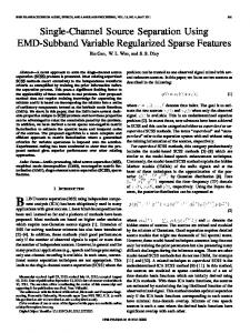
(a) speech
(b) GSN
(c) HCAE
(d) CGBRBM
(e) noise
(f) GSN
(g) HCAE
(h) CGBRBM
(i) ideal softmask
(j) GSN
(k) HCAE
(l) CGBRBM
3.2. Results A grid test on SD data using a GSN over M × d layers, where M ∈ {256, 500, 1000, 2000, 3000} are the neurons per layer and d ∈ {1, 2, 3} was performed to find the optimal network configuration. Sigmoid RBM- and HCAE variants were configured with network size of 2000 × 1. The optimal GSN is a 2000 × 2 network using rectifier activation functions and Gaussian pre- and post activation noise with σ = 0.1, trained with k = 2 × d walkback steps. All models used linear downward activations in the first layer allowing to fully generate the zero-mean and unit variance normalized data. The network weights were initialized with an uniform distribution [36] and trained with early stopping. The mean-squareerror was used as objective function for training all models using single spectrogram frames as input, i.e. frame-wise processing is performed. In particular, we have two models, one maps the mixture to the speech spectrogram, the other one is filtering the interfering signal from the mixture. The softmask is determined from the recovery of both sources. Figure 2 shows a reverberated clean speech spectrogram of the utterance “Place green in b 5 now”, spoken by s20 (2a), a noise spectrogram (2e), and the computed optimal softmask (2i). Speech and noise are mixed at 0dB. Figure (2b), (2f) and (2j) show the reconstructions of speech and noise generated by the GSN, given the mixed signal and the resulting softmask. Figure (2c), (2g) and (2k) show the reconstructions of the HCAE and Figure (2d), (2h), (2l) the reconstructions generated by the CGBRBM, respectively. All models are optimized in a SD fashion. The recovered noise spectrogram is best for HCAE, while the GSN is finding the best representation for the speech spectrogram. The GSN obtains the most similar softmask compared to the optimal mask visually and in terms of the mean square error. The CGBRBM is not able to recover a meaningful temporal structure in the spectrogram. The GSN mostly outperforms the other models with respect to the objective evaluation scores OPS and PESQ. This is shown in Table 2, 3, 4, 5 for the SD, SI, MC, and UC task and different dB conditions, respectively. Furthermore, we present OPS and PESQ scores for the mixed signal and the optimally separated signal using the ideal softmask. In general, networks with multiple layers outperform single layer networks. The frame-wise GSN was able to outperform in most cases any other model including the discriminative MLPs of [10] which use 5 spectrogram frames as input. For the MN and UN tasks the MLPs of [10] achieve sometimes a slightly better PESQ value. Whereas, the MN task uses completely the same noise Ids for both training and testing. This renders this task unrealistic but nevertheless it has been included to be comparable to [9]. For the SD and the SI task the GSN achieves a slightly better PESQ score
Fig. 2: Log-spectrograms of the utterance “Place green in b 5 now” spoken by s20, the noise, and the resulting softmask recovered by various frame-wise SD deep representation models. The first column shows the ideal softmask and the original noise and speech utterance. The remaining columns depict the reconstructions by GSNs, HCAEs, and CGBRBMs, respectively. Model
-6dB
-3dB
mixed signal MLP[10] MLP CGBRBM GBRBM HCAE GSN optimal mask
1.60 1.72 1.72 1.74 1.75 1.77 2.09 4.50
1.85 1.96 1.96 1.98 1.99 2.01 2.30 4.50
mixed signal MLP [10] MLP CGBRBM GBRBM HCAE GSN optimal mask
9.67 10.02 25.25 15.68 9.93 12.20 33.11 98.89
10.34 10.56 26.76 17.05 10.59 24.42 37.44 98.89
0dB
3dB
PESQ 2.08 2.32 2.22 2.44 2.22 2.42 2.21 2.44 2.22 2.46 2.38 2.60 2.53 2.75 4.50 4.50 OPS 11.68 13.81 12.30 14.50 29.31 30.47 18.69 20.81 12.02 14.80 25.72 26.69 42.08 45.34 98.89 98.89
6dB
9dB
2.56 2.63 2.64 2.66 2.67 2.80 2.94 4.50
2.77 2.82 2.84 2.85 2.87 3.01 3.14 4.50
17.31 17.68 32.32 23.22 17.95 27.92 47.59 98.89
21.52 22.84 35.54 27.28 23.26 31.07 50.34 98.89
Table 2: PESQ and OPS results of SD task; Bold numbers denote best results for each specific noise level.
Model
-6dB
-3dB
mixed signal MLP[10] MLP CGBRBM GBRBM HCAE GSN optimal mask
1.37 1.47 1.50 1.37 1.45 1.51 1.62 4.50
1.65 1.66 1.69 1.64 1.70 1.75 1.87 4.50
mixed signal MLP[10] MLP CGBRBM GBRBM HCAE GSN optimal mask
10.02 10.40 10.40 10.16 9.81 13.06 29.25 98.89
10.59 11.02 11.02 11.14 11.15 13.51 33.50 98.89
0dB
3dB
PESQ 1.81 2.07 1.87 2.16 1.90 2.12 1.90 2.12 1.93 2.16 1.99 2.22 2.06 2.29 4.50 4.50 OPS 12.45 14.20 12.27 14.29 12.27 14.29 12.64 14.24 12.60 14.21 14.68 15.63 38.39 42.22 98.89 98.89
6dB
9dB
Model
-6dB
-3dB
2.38 2.36 2.43 2.43 2.44 2.52 2.55 4.50
2.59 2.56 2.64 2.64 2.65 2.71 2.75 4.50
mixed signal MLP [10] MLP CGBRBM GBRBM HCAE GSN optimal mask
1.61 1.73 1.64 1.67 1.65 1.68 1.68 4.50
1.83 1.89 1.84 1.86 1.85 1.79 1.88 4.50
16.70 17.44 17.44 17.13 16.96 17.23 43.21 98.89
21.88 22.74 22.74 22.57 22.13 20.28 45.84 98.89
mixed signal MLP MLP [10] CGBRBM GBRBM HCAE GSN optimal mask
13.93 26.24 26.13 13.06 12.98 22.99 26.63 98.89
16.08 30.80 21.99 14.83 14.91 26.64 31.44 98.89
Table 3: PESQ and OPS results of SI task; Bold numbers denote best results for each specific noise level.
0dB
3dB
PESQ 1.95 2.15 2.08 2.29 2.02 2.20 2.04 2.21 2.05 2.23 2.00 2.21 2.07 2.40 4.50 4.50 OPS 19.58 22.54 35.93 39.60 22.03 26.11 18.28 22.23 18.49 22.43 30.43 33.47 36.46 40.86 98.89 98.89
6dB
9dB
2.35 2.50 2.40 2.40 2.43 2.38 2.51 4.50
2.56 2.73 2.63 2.62 2.64 2.58 2.75 4.50
27.89 42.93 32.23 27.71 28.31 36.59 45.39 98.89
33.77 47.17 41.33 34.26 34.96 40.09 50.42 98.89
Table 5: PESQ and OPS results of UN task; Bold numbers denote best results for each specific noise level. 4. CONCLUSION
for all noise levels. The PESQ is developed for evaluating narrowband speech signal. The OPS of the GSN is significantly better on both tasks. These results indicate that learning deep representations by jointly optimizing multiple layers as performed in GSNs might be beneficial. However, the performance gap to the optimal mask reveals that there is still significant improvement possible. One potential problem might be the generalization potential of all models due to lack of sufficient amount of data. We also performed informal listening tests confirming the results, i.e. utterances processed by GSNs sound more natural and suppress the noise in a better way than the other methods.
Model
-6dB
-3dB
mixed signal MLP [10] MLP CGBRBM GBRBM HCAE GSN optimal mask
1.50 2.44 1.85 1.63 1.72 1.82 2.23 4.50
1.70 2.65 2.04 1.85 1.90 1.96 2.44 4.50
mixed signal MLP [10] MLP CGBRBM GBRBM HCAE GSN optimal mask
9.44 32.85 30.44 9.91 10.05 21.79 34.34 98.89
10.39 35.47 32.98 10.78 10.67 23.42 36.92 98.89
0dB
3dB
PESQ 1.90 2.12 2.83 3.00 2.20 2.40 2.05 2.28 2.09 2.32 2.19 2.36 2.63 2.85 4.50 4.50 OPS 12.36 14.23 39.68 45.97 35.37 38.24 12.60 14.87 12.76 15.45 25.27 29.90 40.53 44.82 98.89 98.89
6dB
9dB
2.43 3.15 2.61 2.48 2.52 2.55 3.06 4.50
2.64 3.30 2.84 2.66 2.70 2.72 3.24 4.50
17.03 51.80 41.35 19.16 19.99 36.66 50.93 98.89
22.15 58.12 48.31 33.00 33.92 45.15 59.32 98.89
Table 4: PESQ and OPS results of MN task; Bold numbers denote best results for each specific noise level.
In this paper, we systematically analyze the effectiveness of representation learning for SCSS. In particular, we evaluated Gauss Bernoulli restricted Boltzmann machines (GBRBMs), conditional Gauss Bernoulli restricted Boltzmann machines (CGBRBMs), higher order contractive autoencoders (HCAEs), and generative stochastic networks (GSNs) on a speaker-dependent (SD), speakerindependent (SI), matched noise condition (MC) and unmatched noise condition (UC) SCSS task using the CHiME and NOISEX database. We applied a two model filtering approach, i.e. training each model separately on mixed spectrograms and the corresponding source representations. GSNs outperform HCAEs, RBMs and also discriminative models, such as multi-layer perceptrons. In future, we extend the models to explicitly model the temporal information. Furthermore, we aim to use more realistic data and larger data sets to obtain a better generalization of the learned representations. This also includes models with more hidden layers. Additionally, formal listening tests are performed. 5. REFERENCES [1] Y. Bengio, “Learning deep architectures for AI,” Foundations and Trends in Machine Learning, vol. 2, no. 1, pp. 1–127, 2009. [2] D. Yu and L. Deng, “Deep learning and its applications to signal and information processing,” IEEE Signal Processing Magazine, vol. 28, no. 1, pp. 145–154, 2011. [3] G. Hinton, L. Deng, G. E. Dahl, A. Mohamed, N. Jaitly, A. Senior, V. Vanhoucke, P. Nguyen, T. Sainath, and B. Kingsbury, “Deep neural networks for acoustic modeling in speech recognition.,” IEEE Signal Processing Magazine, vol. 29, no. 6, pp. 82–97, 2012. [4] G.E. Hinton, N. Srivastava, A. Krizhevsky, I. Sutskever, and R. Salakhutdinov, “Improving neural networks by preventing co-adaptation of feature detectors,” CoRR, 2012.
[5] S.T. Roweis, “Factorial models and refiltering for speech separation and denoising,” in EUROSPEECH, 2003, pp. 1009– 1012. [6] A. Ozerov, P. Philippe, F. Bimbot, and R. Gribonval, “Adaptation of Bayesian models for single-channel source separation and its application to voice/music separation in popular songs,” IEEE Transactions on Audio, Speech, and Language Processing, vol. 15, no. 5, pp. 1564 –1578, 2007.
[21] “ITU-T Recommendation P.862. Perceptual Evaluation of Speech Quality (PESQ): An Objective Method for End-To-End Speech Quality Assessment of Narrow-Band Telephone Networks and Speech Codecs,” Feb. 2001. [22] V. Emiya, E. Vincent, N. Harlander, and V. Hohmann, “Subjective and objective quality assessment of audio source separation,” IEEE Transactions on Audio, Speech, and Language Processing, vol. 19, no. 7, pp. 2046–2057, 2011.
[7] D. D. Lee and H.S Seung, “Learning the parts of objects by nonnegative matrix factorization,” Nature, vol. 401, pp. 788– 791, 1999.
[23] D.H. Ackley, G.E. Hinton, and T.J. Sejnowski, “A learning algorithm for Boltzmann machines,” Cognitive Science, vol. 9, no. 2, pp. 147–169, 1985.
[8] P. Smaragdis, “Convolutive speech bases and their application to supervised speech separation,” IEEE Trans. Audio Speech and Language Processing, vol. 15, no. 1, pp. 1–12, 2007.
[24] P. Smolensky, Information processing in dynamical systems: Foundations of harmony theory, vol. 1, pp. 194–281, MIT Press, 1986.
[9] Y. Wang and D. Wang, “Cocktail party processing via structured prediction,” in Neural Information Processing Systems (NIPS), 2012, pp. 224–232.
[25] T. Tieleman, “Training restricted Boltzmann machines using approximations to the likelihood gradient,” in Intern. Conf. on Machine learning (ICML), 2008, pp. 1064–1071.
[10] M. Z¨ohrer and F. Pernkopf, “Single channel source separation with general stochastic networks,” in International Conference on Spoken Language Processing (Interspeech), 2014.
[26] G.E. Hinton and R.R. Salakhutdinov, “Reducing the dimensionality of data with neural networks.,” Science, vol. 313, no. 5786, pp. 504–507, 2006.
[11] R. Peharz and R. Pernkopf, “On linear and MIXMAX interaction models for single channel source separation,” in International Conference on Acoustics, Speech, and Signal Processing (ICASSP), 2012, pp. 249–252.
[27] G. Hinton, “A Practical Guide to Training Restricted Boltzmann Machines,” Tech. Rep., Department of Computer Science, University of Toronto, 2010.
[12] F. Weninger, F. Eyben, and B. Schuller, “Single-channel speech separation with memory-enhanced recurrent neural networks,” in International Conference on Acoustics, Speech, and Signal Processing (ICASSP), 2014, pp. 3709–3713.
[28] G. Dahl, M. Ranzato, A. Mohamed, and G.E. Hinton, “Phone recognition with the mean-covariance restricted boltzmann machine,” in Neural Information Processing Systems (NIPS), 2010, pp. 469–477.
[13] P.S. Huang, M. Kim, M. Hasegawa-Johnson, and P. Smaragdis, “Singing-voice separation from monaural recordings using deep recurrent neural networks,” in International Society for Music Information Retrieval Conference (ISMIR), 2014, pp. 477–482.
[29] R. Sarikaya, G.E. Hinton, and A. Deoras, “Application of deep belief networks for natural language understanding,” IEEE Transactions on Audio Speech and Language Processing, vol. 22, no. 4, pp. 778–784, 2014.
[14] M. Wohlmayr, L. Mohr, and F. Pernkopf, “Self-adaption in single-channel source separation,” in International Conference on Spoken Language Processing (Interspeech), 2014.
[30] Y. Bengio, P. Lamblin, D. Popovici, and H. Larochelle, “Greedy layer-wise training of deep networks,” in Neural Information Processing Systems (NIPS), 2007.
[15] K. Cho, A. Ilin, and T. Raiko, “Improved learning of GaussianBernoulli restricted Boltzmann machines,” in Intern. Conf. on Artificial Neural Networks (ICANN), 2011, pp. 10–17.
[31] P. Vincent, H. Larochelle, Y. Bengio, and P. Manzagol, “Extracting and composing robust features with denoising autoencoders,” in International Conference on Machine learning (ICML), 2008, pp. 1096–1103.
[16] G.W. Taylor and G.E. Hinton, “Factored conditional restricted Boltzmann machines for modeling motion style,” Intern. Conf. on Machine Learning (ICML), pp. 1025–1032, 2009.
[32] S. Rifai and X. Muller, “Contractive auto-encoders: Explicit invariance during feature extraction,” in International Conference on Machine learning (ICML), 2011, pp. 833–840.
[17] S. Rifai, G. Mesnil, P. Vincent, X. Muller, Y. Bengio, Y. Dauphin, and X. Glorot, “Higher order contractive autoencoder,” in European Conference on Machine Learning and Principles and Practice of Knowledge Discovery in Databases (ECML PKDD), 2011.
[33] G. Alain, Y. Bengio, and S. Rifai, “Regularized auto-encoders estimate local statistics,” CoRR, pp. 1–17, 2012.
[18] Y. Bengio, E. Thibodeau-Laufer, and J. Yosinski, “Deep generative stochastic networks trainable by backprop,” in International Conference on Machine Learning (ICML), 2014. [19] M. Z¨ohrer and F. Pernkopf, “General stochastic networks for classification,” Neural Information Processing Systems (NIPS), 2014. [20] E. Vincent, J. Barker, S. Watanabe, J. Le Roux, F. Nesta, and M. Matassoni, “The second CHiME speech separation and recognition challenge: An overview of challenge systems and outcomes,” in Automatic Speech Recognition and Understanding (ASRU) Workshop, 2013.
[34] Y. Bengio, L. Yao, G. Alain, and P. Vincent, “Generalized denoising auto-encoders as generative models,” in Neural Information Processing Systems (NIPS), 2013, vol. 26, pp. 899–907. [35] M. Cooke, J. Barker, S. Cunningham, and X. Shao, “An audiovisual corpus for speech perception and automatic speech recognition.,” The Journal of the Acoustical Society of America, vol. 120, no. 5, pp. 2421–2424, 2006. [36] X. Glorot and Y. Bengio, “Understanding the difficulty of training deep feedforward neural networks,” in International Conference on Artificial Intelligence and Statistics (AISTATS), 2010, pp. 249–256.