Nonlinear Face Recognition based on Maximum Average Margin ...

Nonlinear Face Recognition based on Maximum Average Margin Criterion Baochang Zhang1, Xilin Chen1,2, Shiguang Shan2, Wen Gao1, 2 1

2

Computer School, Harbin Institute of Technology, China ICT-ISVISION Joint R&D Lab for face recognition, ICT, CAS, China {Bczhang, Xlchen, Sgshan, Wgao}@jdl.ac.cn Abstract

This paper proposes a novel nonlinear discriminant analysis method named by Kernerlized Maximum Average Margin Criterion (KMAMC), which has combined the idea of Support Vector Machine with the Kernel Fisher Discriminant Analysis (KFD). We also use a simple method to prove the relationship between both kernel methods. The difference of KMAMC from traditional KFD methods include (1) the within-class and between-class scatter matrices are computed based on the support vectors instead of all the samples; (2) multiple centers are exploited instead of the single center in computing the two scatter matrices; (3) the discriminant criteria is formulated as subtracting the trace of within-class scatter matrix from that of the between-class scatter matrix, therefore, the tedious singularity problem is avoided. These features have made KMAMC more practical for real-world applications. Our experiments on two face databases, the FERET and CAS-PEAL face database, have illustrated its excellent performance compared with some traditional methods such as Eigenface, Fisherface, and KFD. Key Words: Face Recognition, Kernel Fisher, Support Vector Machine

1. Introduction Principle Component Analysis (PCA) and Fisher Linear Discriminant Analysis (FDA) are two classical techniques for linear feature extraction. In many applications, both methods have been proven to be very powerful. However, they are inadequate to describe the complex nonlinear variations in the training dataset. In recent years, the kernelized feature extraction methods have been paid much attention, such as Kernel Principal Component Analysis (KPCA)[1] and Kernel Fisher Discriminant analysis (KFD) [2, 3], which are well-known nonlinear extensions to PCA and FDA respectively. However, the KFD cannot be easily used in real applications. The reason is that the projection directions of KFD often lie in the span of all the samples [5], therefore, the dimension of the feature often becomes very large, when the input space is mapped to a feature space through a kernel function. As a result, the scatter matrices become singular, which is the so-called “Small Sample Size problem” (SSS). Similar to [4], KFD simply adds a perturbation to within-class scatter matrix. Of course, it has the same stability problem as that in [4], because eigenvectors are sensitive to the small

perturbation, moreover, the influence of which is not yet understood. In recent years, many researchers have proposed many methods to overcome the computational difficulty with KFD. Jian Yang [5] used the KPCA + FDA method, a two-stage procedure is employed after the KPCA method has been used to reduce the dimensionality of the original input data. First, one transformation space is extracted from the within-class scatter matrix, which is used to modify the original between-class scatter matrix. Second, it tries to maximize the new between-class scatter matrix by using PCA method. The KPCA generally cannot achieve better performance than PCA [5, 20], and it seems that the proposed scheme is not as effective as the PCA+FDA linear discriminating analysis method. Wei Liu [6] proposed the Nullspace based KFD method (NKFDA), an extension to Nullspace FDA. It first calculates the Null space of within-class scatter matrix, and then modifies the between-class scatter matrix and gets the whole transformation matrix. NKFDA solves the SSS problem, however, the algorithm first calculates the Nullspace of within-class scatter matrix, which is a very difficult task. Moreover, the traditional KFD method is the single-center method, which means that each class during the training process is represented as a single class center, i.e. the sample mean of the class. In this paper, we propose a simple and effective method to make discriminant analysis, which tries to measure the Average Distance between different Margins of SVM by calculating the Euclidean distance between the mean support vectors. Our method is the multi-center approach, and it is based on the support vector set represented by a group of mean sample vectors. In the paper [18], Bernhard showed that using the support vectors can achieve full performance of the classifier trained by using all the samples, therefore, we can know that support vectors are strongly related to the classification task. Rik Fransens[19] combined the normal directions idea with SVM classifier, which only utilized the support vectors and achieved good result in its application of face detection. Moreover, the new criterion does not suffer from the SSS problem, which is known as the serious stability problem for Fisher Criterion. We apply the proposed method to the face recognition problem, which is one of hot points in the field of pattern recognition [7]. The rest of the paper is organized as following. In Section 2, KMAMC is proposed to make nonlinear discriminant analysis for the original input image. In Section 3, we will conduct some experiments on CAS-

PEAL and FERET databases to evaluate the performance of the proposed method. In the last Section, we will make some conclusions about the experiment results.

where

2. Kernelized Criterion

1 n , 1 n 1 n mi =  ∑ji=1 k( x1 , x j ), ∑ji=1 k( x2 , x j ),.., ∑ji=1 k( xn , x j )  ni ni  ni 

C

_

_

K b = ∑ p(ϖ i )(mi − m)(mi − m) T

,

(8)

i =1

η j = (k ( x1 , x j ), k ( x 2 , x j ),..., k ( x n , x j )) T

,

_

Maximum Average Margin

We first describe the Kernel Fisher analysis method, which is a well-known extension to FDA. Moreover, many definitions will be used in our paper later, such as the kernel within-class and between-class scatter matrices. It is also the baseline algorithm in our paper, and we will make some comparative experiments with the proposed method.

2.1 Kernel Fisher Discriminant Analysis The idea of Kernel FDA is to yield a nonlinear discriminant analysis in a higher dimensional space. The input data is first projected into an implicit feature space F by the nonlinear mapping Φ : x ∈ R N − > f ∈ F , and then seek to find a nonlinear transformation, which can maximize the between-class scatter and minimize the within-class scatter in F [5]. In its implementation Φ is implicit and we will just compute the inner product of two vectors in F by using a kernel function: (1) k ( x , y ) = ( Φ ( x ) ⋅ Φ ( y )) . We define between-class scatter matrix

S b and within-

S w in the feature space F as

class scatter matrix following: C

S b = ∑ p(ϖ i )(ui − u)(ui − u) T ,

(2)

i =1

C

SW = ∑ p(ϖ i ) E{((Φ ( xi ) − ui )(Φ( xi ) − ui )T ) | ϖ i }

,

(3)

i =1

ui =

1 ni

ni

∑φ ( x j =1

ij

)

denotes the sample mean of class i , and

u

is the mean of all training images in F , p (ϖ i ) is the prior probability. To perform FDA in a higher dimensional space F , it is equal to maximize Eq.4. wT Sb w tr(Sb ) . (4) J (w) =

mean of all

and

m is the

ηj.

Similar to FDA [4,10], this problem can be solved by finding the leading eigenvectors of K −w1K b used by Liu [8] and Baudat (GDA)[3], which is the Generalized Kernel Fisher Discriminant (GKFD) criterion. In our paper, we use the technique of the pseudo inverse of the within-class scatter matrix, and then perform PCA on K −w1K b to get the transformation matrix α . The projection of a data point x onto w in F is given by: n (9) v = ( w . Φ ( x ))

=

∑

α

i

k ( x

i

, x )

i = 1

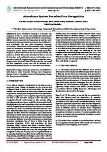
2.2 the Property of SVM Support Vector Machines (SVM) is a state-of-the-art pattern recognition technique, whose foundations stem from the statistical learning theory. However, the scope of SVM is beyond pattern recognition because they can also handle another two learning problems, i.e., regression estimation and density estimation. SVM is a general algorithm based on guaranteed risk bounds of statistical learning, the so-called structural risk minimization principle. And we can refer to the tutorials [9,12] about the SVM. The success of SVM in face recognition [13, 14] as a recognizer provides us with further motivation to utilize SVM to enhance the performance of our system. However, we did not construct SVM classifier, and just used it to find the support vectors shown in Fig.1. Here, we will use a simple way to prove the property of support vectors based within-class scatter matrix for twoclass problem, which shows that SVM is strongly related to the Kernel Fisher analysis method.

= wT Sww tr(Sw )

Because any solution w ∈ F should lie in the span of all the samples in F [8], there exists: n (5) w = α φ ( x ), α , i = 1,2...n. .

∑ i =1

i

i

i

Then we will get the following Maximizing Criterion: (6) α T K bα , J (α ) =

where

α T K wα

K w and K b are defined as following: C

Kw = ∑ p(ϖi )E(η j − mi )(η j − mi )T i =1

,

(7)

Fig.1 Support Vectors are circled such as

x1 , x 2

In a higher dimensional space, x1 , x 2 are represented as Φ ( x1 ), Φ ( x 2 ) . The SVM aims to optimize the following objective function [9,12]: 1 T , (10) w w Min w

2

Subject to: yi ( w Φ( xi ) + b) − 1 ≥ 0 . T

(11)

Here, if Φ( xi ) is the support vector, we can know that[9]: (12) y i ( wT Φ( xi ) + b) − 1 = 0, y i ∈ {−1,1} .

belonging to the class i , and the other is S i 2 including all

Thus, for Φ ( x1 ), Φ( x 2 ) are the support vectors, we have: wT Φ( x1 ) + b = 1, Φ( x1 ) ∈ S1 , , (13)

set Si1 , and p (ϖ i ) is the prior probability. u 'j 0 denotes

S1 = {Φ( xi ) | yi = 1, wT Φ( xi ) + b = 1} wT Φ ( x 2 ) + b = −1, Φ ( x2 ) ∈ S 2 ,

.

(14)

The elements of S1 and S 2 are support vectors, and it is easy for us to prove the following equations: , (15) ____

w T Φ ( x1 ) = 1 − b, 1 n1

∑ Φ ( x), Φ ( x) ∈ S

1 n2

only one sample for one class is contained in the sample is the class center). And now

,

∑ Φ ( x ), Φ ( x) ∈ S

(16)

( | Cm style

1

i = 1, Φ ( x i )∈ S 1

n2

∑ (Φ ( x

i =1, Φ ( x i )∈ S 2

____

i

____

T

) − Φ ( x 2 ) )( Φ ( x i ) − Φ ( x 2 ))

Therefore, we can know that: (18) w T S 'w w = 0 , ' where S w is the within-class scatter matrix calculated by using the support vectors. w is related to the centers of two classes taken from the set of support vectors. For multi-class problem, we redefine the between-class scatter matrix S 'b and within-class scatter matrix S 'w based on the

support vector set, calculated in the SVM by using the ‘one to rest’ strategy. C 1 n ' , (19) S' = p(ϖ ) (u − u ' )(u ' − u ' )T b

c

∑ i =1

S'w = ∑ p (ϖ i ) i =1

K ,K ' w

' B

i

i

∑ n +1 i

i

k =0

c

∑ p(ϖ

m

S i can be

jk

' j0

calculate the within-class scatter sub-matrix for the class, if more than one samples of which are contained in S i

2

class problem, the within-class scatter matrix is defined as following: T n ____ ____ n1 (17) S 'w = ∑ ( Φ ( x i ) − Φ ( x1 )) ( Φ ( x i ) − Φ ( x 1 )) + . n2 n 2 + n1

S i 2 , then

so we can know u m' ∈ {u i' , u 'j 0 , u 'j1 ,..., u 'jn } . We will i

n1 is the size of the S1 , n2 is the size of the S2 . For two-

n 2 + n1

ni , and

represented by a multi-center vector (u , u , u 'j1 ,..., u 'jn i ) ,

1

____

____

different classes. The number of classes in S i 2 is

' i

w T Φ ( x 2 ) = − 1 − b, Φ(x2 ) =

the sample mean of S i 2 , whose samples come from the center of the class is represented as u , k = 1,.., ni (if

S 2 = {Φ ( xi ) | y i = −1, w Φ ( xi ) + b = −1}

____

ui' denotes the sample mean of the

' jk

T

Φ ( x1 ) =

other support vectors.

i

jk

| ϖ i )E ((Φ ( xm' ) − um' )(Φ( xm' ) − um' )T )

.

m =1, C m ∈S i ,|C m |>1, x m' ∈C m

(20) are calculated just like Eq.7 and Eq.8. The

traditional Fisher discriminating analysis is a single-center method in the sense that each class during training process is represented by a single example (generally the mean sample vector), therefore, our method can be thought as a muti-center method, because we use several mean sample vectors to represent each support vector set. In the case that only samples of Ci are included in the positive set, and other samples are included in the negative set for twoclass SVM algorithm, we will explain the parameters used in Eq.19 and Eq.20 as following. Si includes all the support vectors, which is divided into two sub-sets, one of which is Si1 , whose elements are the support vectors

|> 1

). In our paper, the kernel function is polynomial

used

in

SVM and the proposed r is a constant integer.

method,

, x⋅ y k ( x, y ) = ( + 1) r | x |⋅| y |

To be concluded, in this part, we get the new withinclass and between-class scatter matrices based on the support vector set, which is represented by a multi-center vector, (u i' , u 'j 0 , u 'j1 ,..., u 'jn ) . i

2.3 Maximum Average Margin Criterion From the above discussion, we know that the support vectors have good properties. In this part, some distance metric is used to measure the dissimilarity between different classes based on the support vectors. We hope that the transformation matrix should maximize the distance between the Margins of the SVM, data points of which are strongly related to the classification task. Simply, considering the two-class problem, we use Ci and C 'j to represent the support vector sets, whose samples

come from the different Margins. Now, we define the maximizing criterion as following: C . (21) ' J =

∑

i =1

p (ϖ i ) d ( C i , C j )

We call it Maximum Average Margin Criterion (MAMC), actually we can use some distance measure between the mean support vectors as the distance between the Margins. (22) d (Ci , C 'j ) = d (ui' , u 'j ) , where u i' is the mean vector of support vectors in the data set Ci , u 'j is the mean vector of the remained support vectors in C 'j . By employing the Euclidean distance, we can also represent Eq.21 as following:

J =

C

∑

i =1

p (ϖ i )( u 'i − u 'j ) T ( u 'i − u ' j )

,

(23)

C

= tr ( ∑ p (ϖ i )( u 'i − u 'j )( u 'i − u ' j ) T ) i =1

We know that C 'j includes the samples coming from different classes, which is represented as a multi-center vector, and then the maximizing criterion is redefined as following: C 1 n ' J = tr ( p (ϖ ) (u − u ' )(u ' − u ' )T ) = tr (S ' ) . (24)

∑ i =1

i

i

∑

ni + 1 k = 0

i

jk

i

jk

b

Here, Eq.24 is equal to the Eq.19. According to the Fisher criterion, we also hope that the within-class scatter should be minimized. If our criterion maximizes the distance between mean support vectors, at same time, minimizes the scatter of classes, we can know that it will almost be consistent with the Fisher criterion. Therefore, we redefine the Criterion by considering the trace of the within-class scatter matrix as following: (25) J = tr ( S 'b ) − tr ( S w ) . We also hope that the transformation matrix has the same property as in the SVM, and some constraint function can be used here. Because the distance between the Margins is used to measure the distance between different classes, so the function utilized to constraint Eq.25 should be related to the support vectors, for example, Eq.18 is very suitable in this situation. Now, we obtain the objective functions as following: (26) Max: J = tr ( S b' − S w ) , T ' Subject to: w S w w = 0 , (27)

where S w and S'w are defined in Eq.3 and Eq.20. Since the tr (S b' ) measures the average distance between margins of SVM, a large tr (S b' ) implies that the support vectors are far from each other if they are from different classes. On the other hand, a small tr ( S w ) based on all samples denotes for every class having a small variance. Thus a large J indicates that the nearest data points in the different classes are in a large space and the classes have small overall variance. Moreover, the constraint function has been used for MAMC, which are strongly related to the classic algorithm of SVM. In a higher dimensional space F , considering the so-called KMAMC, we have objective functions as following: Max: J = tr ( K 'b − K w ) , (28) (29) Subject to: α T K 'w α = 0 . In the following part, we will use a simple method to optimize the above objective functions.

2.4 The Algorithm of KMAMC The KMAMC improves the generalization capability by decomposing its procedure into a simultaneous

diagonalization of two matrices. The simultaneous diagonalization is stepwisely equivalent to two operations, and we first whiten K b' − K w as following:

( K 'b − K w )Ξ = ΞΓ and Ξ Ξ = Ι , T

Γ

−1 / 2

Ξ (K − K w )ΞΓ T

' b

−1 / 2

= Ι,

(30) (31)

where Ξ , Γ are the eigenvector and the diagonal eigenvalue matrices of K b' − K w . We can get the eigenvectors matrix Ξ , whose eigenvalues are bigger than zero (Corresponding diagonal eigenvalue matrix is '

Γ' −1 / 2 ), and tr (K 'b ) is always bigger than tr (K w ) . The new within-class scatter matrix is computed by using the following method: (32) Γ' −1/ 2Ξ'T K 'wΞ' Γ' −1/ 2 = Ξ w . Diagonalizing now the new within-class scatter matrix Ξ w .

Ξ w θ = θγ and θ T θ = I ,

(33)

where θ , γ are the eigenvector and the diagonal eigenvalue matrices of Ξ w in an increasing order. We get rid of the Eigenvectors, whose eigenvalues are far from zero, and the remained Eigenvectors construct the transformation matrix θ . The overall transformation matrix is now defined as following. '

α ' = Ξ ' Γ ' −1 / 2 θ ' . We use w ' as the transform matrix, feature calculated by using Eq.35 v = w

'

Φ ( x ) =

n

∑

i = 1

α

' i

(34)

v is the extracted

k ( x i, x ) .

(35)

2.5 Similarity Measure for KMAMC If v 1 , v 2 are the feature vectors corresponding to two face images x 1 , x 2 , which are calculated by using the Eq.35, then the similarity rule is based on the cross correlation between the corresponding extracted feature vectors as following: (36) v 1 .v 2 d ( x1 , x 2 ) =

|| v 1 || . || v 2 ||

Experiments are performed on two databases, CAS-PEAL and FERET databases. Comparative performance is carried out against the Eigenface, Fisherface, NKFDA and GKFD.

3. EXPERIMENT In our experiments, the face image is cropped to size of 64X64 and overlapped with a mask to eliminate the background and hair. For all images concerned in the experiments, no preprocessing is exploited. To speed up

the system, we first make PCA on the face images, and the lower dimensional vector in the PCA space is used in our experiments to capture the most expressive features of the original data.

3.1 CAS-PEAL Database The CAS-PEAL face database was constructed under the sponsors of National Hi-Tech Program and ISVISION[17]. The goals to create the CAS-PEAL face database include: providing the worldwide researchers of FR community a large-scale face database for training and evaluating their algorithms; facilitating the development of FR by providing large-scale face images with different sources of variations, especially Pose, Expression, Accessories, and Lighting (PEAL); advancing the state-ofthe-art face recognition technologies aiming at practical applications especially for the oriental. Currently, the CAS-PEAL face database contains 99,594 images of 1040 individuals (595 males and 445 females) with varying Pose, Expression, Accessory, and Lighting (PEAL). Gallery set contains one image for each person. One sample person was shown in Fig.2, and the size of the face image is 360X480. In this experiment, only one face image for each person was used as Gallery database, whose identity is known to the system. Details of the face database are shown at http://jdl.ac.cn/peal/index.html[17].

Fig.2. Sample of Face Images in CAS-PEAL database Table1. Experiment Result on CAS-PEAL database (Accurate rate)

Fisherface method refers to EFM-2[11], r=2 Eigenface Accesso ry Backgro und Distanc e Expressi on Aging

Fisherface

NKFDA

GKFD

KMAMC

37.1

61

61.5

58.7

64.3

80.5

94.4

94

91.7

94.6

74.2

93.5

93.8

94.9

96

53.7

71.3 72.7

77.5 83.3

78.2 77.3

82.5

50

86.4

3.2 FERET Database The proposed algorithm is also tested on a subset of the FERET face image database. This subset includes 1400 images of 200 individuals, and each individual has 7 images.

It is composed of images named with two-character strings, ”ba”,”bj”,”bk”,”be”,”bd”,”bf” and “bg”. This subset involves variations in facial expression, illumination, and pose. Two groups of experiments are conducted on this subset to evaluate the performance of the propose methods in terms of the mean recognition rate by using the cross-validation method. 100 subjects with 7 images per subject are randomly selected as the training set to calculate the weight vector. And the other 100 subjects are used for the test set, where the images in the 'ba' part are used as gallery, and 6 images per subject from the other parts ('bj', 'bk', 'be', 'bf', 'bd', and 'bg') are used as the probe set.

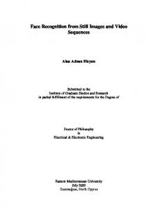
Fig.3. Sample of Face Images in FERET database 90 80 70 60 50 40 30

PCA Fisherface GKFD NKFDA KMAMC

Chart1. Experiment Results on FERET database, r=2

From the above experiments, we can know that the proposed method is better than all other methods. Fisherface is sometime better than GKFD, since the EFM2[11] approach removes the noise by performing the PCA method on the original input image and the within-class scatter matrix. NKFDA is better than the GKFD method, the reason for which may be that GKFD reserves the noise when adding the perturbation to the within-class scatter matrix. The KMAMC is the multi-center method, which can reserve more information than the tradition Fisher analysis approach, at same time, it is implemented by using the PCA method, which can help to reserve the useful information and remove the noise from the training data set.

4. Conclusion and Future Work We have proposed a novel nonlinear discriminant analysis method named by Kernerlized Maximum Average Margin Criterion. The new method does not suffer from the ‘SSS’ problem and it is easily realized in its application. We also utilize a simple method to prove the property of the SVM, which is used as a constraint function for the KMAMC. Specially, the new within-class and between-class scatter matrices are defined based on the support vector set by using the multi-center method, and the traditional Fisher is the single-center method in the sense that each class during training process is represented by a single mean sample vector. The

feasibility of the new method has also been successfully tested on face recognition problem using data sets from the FERET database, which is a standard testbed for face recognition technologies, and CAS-PEAL database, which is a very large one. The effectiveness of the method is shown in terms of accurate rate against some popular face recognition schemes, such as Eigenface, Fisherface, GKFD, and so on. Gabor wavelet feature has been combined with some discriminant methods and successfully used in the face recognition field [15, 16]. Therefore, we try to make full use of Gabor wavelet representation of face images before using KMAMC to get the transformation matrix. Another possibility is to increase the generalization ability of the learning classification machine minimizing the empirical risk encountered during training and narrowing the confidence interval for reducing the guaranteed risk while testing on unseen data.

5. Acknowledgement This research is partially sponsored by Natural Science Foundation of China under contract No.60332010 "100 Talents Program" of CAS, ShangHai Municipal Sciences and Technology Committee (No. 03DZ15013), and ISVISION Technologies Co., Ltd.

Reference [1]B. Scholkopf, A. Smola, K.R. Muller, “Nonlinear component analysis as a kernel eigenvalue problem,” Neural Computation, vol.10, pp.1299-1319, 1998. [2]S. Mika, G. Ratsch, J. Weston, B. Scholkopf and K.R. Muller, "Fisher discriminant analysis with kernels, " IEEE International Workshop on Neural Networks for Signal Processing, pp.41-48, 1999. [3]G. Baudat, F. Anouar, "Generalized discriminant analysis using a kernel approach, " Neural Computation, vol.12, no.10, pp.2385-2404, 2000. [4]Z. hong and J. Yang, "Optimal discriminant plane for a small number of samples and design method of classifier on the plane, " Pattern recognition, vol.24, no.4, pp.317324, 1991. [5]Jian yang, Alejandro, "A new Kernel fisher discriminant algorithm with application to face recognition," Letters of Neurocomputinting, 2003. [6]Wei Liu, Yunhong Wang, "Null space based Kernel Fisher Discriminant analysis for face recognition," The 6th International Conference on Automatic Face and Gesture Recognition, 2004. [7]R. Chellappa, C.L. Wilson, and S. Sirohey, "Human and machine recognition of faces: A survey," Proc. IEEE, vol. 83, no. 5, pp.705-740, 1995. [8]Qingshan Liu, Rui Huang, "Face Recognition Using Kernel Based Fisher Discriminant Analysis, " The 5th

International Conference on Automatic Face and Gesture Recognition, pp.187-191, 2002. [9]K. Fukunaga, Introduction to Statistical Pattern Recognition, Academic Press, second edition, 1991. [10]K. Etemad and R. Chellappa, "Discriminant analysis for recognition of human faces," Proceedings of the First International Conference on Audio- and Video-Based Biometric Person Authentication, pp.127-142, 1997. [11]Chenjun liu, Harry Wechsler, "Enhanced Fisher Linear Discriminant Models for face Recognition," 14th International Conference on Pattern Recognition, vol.2, pp.1368-1372, 1998. [12]C.J.C. Burges, "A tutorial on support vector machines for pattern recognition,” Knowledge Discovery and Data Mining, vol.2, pp.121-167, 1998. [13]G. Guo, S.Z. Li, and C. Kapluk. "Face recognition by support vector machines," Image and Vision Computing, vol.19, pp.631--638, 2001. [14]A. Tefas, C. Kotropoulos, and L. Pitas, "Using Support Vector Machines to Enhance the Perfornance of Elastic Graph Matching for Frontal Face Authentication, " IEEE Trans. on PAMI, Vol. 23, No. 7, pp.735-746, 2001. [15]Chengjun Liu and Harry Wechsler, "Gabor Feature Based Classification Using the Enhanced Fisher Linear Discriminant Model for Face Recognition, " IEEE Trans. Image Processing vol.11 no.4, pp.467-476, 2002. [16]Baochang Zhang, Wen Gao, Shiguang Shan, Yang Peng, "Discriminant Gaborfaces and Support Vector Machines Classifier for Face Recognition, " Asian Conference on Computer Vision, pp.37-42, 2004. [17]Wen Gao, Bo Cao, Shiguang Shan, "The CAS-PEAL Large-Scale Face Database and Evaluation Protocols," Technical Report No. JDL_TR_04_FR_001, JDL, CAS, 2004. [18]Bernhard Scholkopf, Chris Burges, "Extracting Support Data for a Given Task, " KDD, pp.252-257,1995. [19]Rik Fransens, Jan De Pris, "SVM-based Nonparametric Discriminant Analysis, An application to a Face Detection," ICCV, 2003. [20]Chenjun Liu, "Gabor-based Kernel with Fractional Power Polynomial Models for Face Recognition, " IEEE PAMI, vol.26, pp.572-581,2004.