Several observer design approaches have been proposed in ... established concepts (Patton et al, 1989) for linear ... NONLINEAR OBSERVER DESIGN.
Nonlinear observer-based fault detection Kondo ADJALLAH, Didier MAQUIN, José RAGOT Institut National Polytechnique de Lorraine Centre de Recherche en Automatique de Nancy - CNRS UA 821 BP 3 - 2, Avenue de la Forêt-de-Haye France - 54 516 Vandoeuvre Cedex
Abstract - This communication
deals with t h e problem of designing a nonlinear observer i n order to achieve fault detection and l o c a l i z a t i o n for a wide class of nonlinear systems s u b j e c t e d to bounded nonlinearities. A dedicated n o n l i n e a r observer scheme (DNOS) for fault detection and identification in reconstructible systems is proposed.
INTRODUCTION
State observation of nonlinear dynamical systems is becoming a growing topic of investigation in the specialized literature. The reconstruction of the time behaviour of state variables remains a major problem both in control theory and process diagnosis. Researchers attention is being particularly focused on the design of adaptive observers for on-line process state estimation. There is increasing awareness that to ensure robustness in performance requires simpler and stable adaptive observer schemes. Linear systems have received considerable attention (Luenberger, 1966), (O'Reilly, 1983) leading to several stable adaptive observer systems (Kreisselmeier, 1977, 1979), (Magni and Mouyon, 1991). Linear observer systems involving unknown inputs have also been developed and analyzed (Viswanadham and Srichander, 1987). Nevertheless, the design of asymptotically stable observers remains a hard task in the nonlinear case, even when the nonlinearities are fully known. Several observer design approaches have been proposed in recent years for nonlinear systems. Walcott and Zak (1986) and (1987) for instance, proposed a new type of observer for systems subjected to bounded nonlinearities or uncertainties. This type of observer does not require exact knowledge of the system nonlinearities. Bastin and Gevers (1988) also described an adaptive observer/identifier, for SISO observable nonlinear systems, capable of state estimation and parameter adaptation. Marino (1990) also developed the same idea and proposed a simpler observer restricted however to a class of systems with constant unknown parameters. As a main result, the construction of an observer may be performed by finding suitable state space and output changes of coordinates to transform the nonlinear system into an observable form from which can be derived an observer with linear dynamics. Xia and Gao (1988) and Krener and Isidori (1983) have given Lie algebraic and rank conditions for nonlinear process observability and observer existence purpose. Simultaneously, the techniques of fault detection and isolation (FDI) are increasingly discussed in both research
and applications. It is based on the use of analytical redundancy. The general procedure first generates the socalled residuals (i.e., faults accentuated functions) before proceeding to fault detection and isolation (i.e., determination of its location, duration, type, magnitude, source). The use of observers is among the wellestablished concepts (Patton et al, 1989) for linear systems. For the general case of nonlinear systems (Hengy and Frank, 1986), (Seliger and Frank, 1991) little has so far been achieved in the development of associated FDI observers. Solutions so far proposed are difficult to apply in real situations. This note is organized into four sections. The first presents the observer design for nonlinear systems. The second considers dedicated observers while the third deals with the analysis of generated residuals. The last section is devoted to computational aspects and uses the numerical results of a synchronous machine to highlight the strategy employed to isolate faults. 1. NONLINEAR OBSERVER DESIGN
We shall consider nonlinear systems of the form: ˙ = f ( x(t), u(t)), x(0) = x 0 x(t) y(t) = Cx(t) x∈
(1)
R n , u ∈ R m and y ∈ R p
It is assumed that for any input u(t) and initial state x 0 , the corresponding state trajectory x(t) is defined for all t and that f is continuously differentiable. Proceeding by analogy to the classical observer design approach in the linear case, we seek an observer of the following form: xˆ˙ = f ( xˆ (t), u(t)) + g( y(t)) − g( yˆ (t)), xˆ (0) = xˆ 0 , (2) yˆ = Cxˆ (t) where the analytical function g: R p → R n is to be determined. The state and output errors are respectively defined by: e(t) = x(t) − xˆ (t) ε (t) = y(t) − yˆ (t)
(3)
For a sake of simplicity, the time variable will be now omitted. The dynamic of estimation error e(t) is then:
e˙ = f ( x, u) − f ( xˆ , u) − g( y) + g( yˆ )
(4) So, let us consider the quadratic Lyapunov function:
Assuming that the observer state converges asymptotically to the state of the system, one can consider the state error (equation (3)) in the neighbourhood of zero. This allows the use of a first order Taylor expansion of the function f: f ( x, u) = f ( xˆ + e, u) = f ( xˆ , u) + Dxˆ ( f )e
(5a)
∂ f ( x, u) ∂x T
Similarly, for g: (5b)
with: Dy (g) =
∂ g( y) ∂yT
Consequently, the dynamic of the estimation error may be rewritten:
[
]
(6)
For state reconstruction, the idea is to select a continuous mapping g(y) so that xˆ (t) becomes a state estimator of the process under consideration. If the pair { Dxˆ ( f ), C} is observable at any time t, then a matrix D y (g) must be determined so that (6) has arbitrary stable poles at each operating point parametrized by the control u. The natural question that arises is when does the function g exist ? Only sufficient condition may be found (Misawa and Hedrick, 1989). A particular structure of the observer is proposed in order to simplify the calculation of this mapping: xˆ˙ = f ( xˆ , u ) + R( xˆ , u )( y − yˆ ), xˆ (0) = xˆ 0 (7) yˆ = Cxˆ
V˙ (e) = e T Pe˙
e˙ = f ( x, u) − f ( xˆ , u) − R( xˆ , u )( y − yˆ )
(8)
The matricial function R( xˆ , u ) is chosen so that the state error e(t) asymptotically decreases and approaches zero as t tends to infinity. The error e(t) is then considered to be in the neighbourhood of zero. By using (5a) and (5b), a first order Taylor expansion of the function f(x, u) in the neighbourhood of the estimated state trajectory xˆ (t) is substituted in (8), that gives:
]
e˙ = Dxˆ ( f ) − R( xˆ , u )C e
]
(9)
(11)
This condition ensures that e decreases exponentially to zero (Ogata 1970, Corless 1988). For a particular structure of the function f, Tsinias (1989) proposed an algorithm for determining the gain R( xˆ , u ) based on the assumption that {Ker ( C )} ≠ {0}. We propose here a generalization of this algorithm which is based on a sequential determination of P and R( xˆ , u ) avoiding the nonlinear coupling appearing in (8). The algorithm comprises two steps, the first one being devoted to the determination of P and the second one to the determination of R( xˆ , u ) using the previous value of P. Step 1: If e ∈ is reduced to:
{Ker ( C )} − {0} ,
then the equation (11)
V˙ (e) = e T PDxˆ ( f )e
(12)
The problem is to find a matrix P which ensures the condition: V˙ (e) = e T PDxˆ ( f )e < 0
(13)
Solving inequation (13) yields a value for P . For that purpose, assuming {Ker ( C )} ≠ {0} , one can use the transformation: e = Ke
(14)
where K is right orthogonal to C . Substituting (14) into (13) gives: V˙ (e) = e T K T PDxˆ ( f )Ke
The state error is then solution of the equation:
[
where P is a positive definite matrix. We require time derivative of V(e) to be negative:
y = yˆ
e˙ = Dxˆ ( f ) − Dy (g)C e
(10)
[
x = xˆ
g( y) = g( yˆ ) + Dy (g)Ce
1 T e Pe 2
V˙ (e) = e T P Dxˆ ( f ) − R( xˆ , u )C e
where Dxˆ is a differential operator defined by: Dxˆ ( f ) =
V (e) =
(15)
where the dimension of e is less than those of e. Making V˙ (e) negative, by majorization techniques, gives the matrix P (see the example of section 4). Step 2: If step 1 produces a suitable P , else P can be chosen as an identity matrix, we now allow e ∈ R n and try to determine R( xˆ , u ) which verifies the following inequality:
[
]
V˙ (e) = e T P Dxˆ ( f ) − R( xˆ , u)C e < 0
(16)
A sufficient condition to fulfill this inequality is that the matrix Dxˆ ( f ) − R( xˆ , u)C be negative semidefinite.
This is achieved by using first the following structure proposed for R( xˆ , u): R( xˆ , u) = P −1 F( xˆ , u )C T Q
u(t)
f
(17)
e T PDx ( f )e < e T F( xˆ , u )e
(19)
Secondly, assuming that such a map exists, then using equation (18), one can write: V˙ (e) ≤ e T PDxˆ ( f )e − e T F( xˆ , u )Dxˆ (h)T QDxˆ (h)e (20) According to inequality (19) we say that a sufficient condition for satisfying the Lyapunov stability condition (13) can be summarized as follows: find a (p, p) matrix Q such that the map C T QC − I be positive semidefinite. All positive defined matrix F(x, u) that verifies the inequality
[
]
PDx ( f ) < F( x, u ) fulfill the inequality (19). The matricial norm is those induced by the Euclidean vector norm . . We then propose for F(x, u) the following map: F( x, u ) = diag( φ i ( x, u)) where diag defines a diagonal matrix in which the diagonal elements are defined by: φ i ( x,
u) =
1 n ∑ α ij ( x, u) + α ji ( x, u) 2 j=1
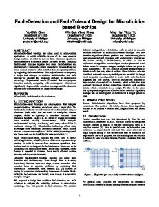
where α ij are the elements of PDx ( f ). To summarize, the existence of P , verifying inequation (13), and those of Q verifying (20) are the two conditions needed to design the state observer (2) which is described by: xˆ˙ = f ( xˆ , u) + P −1 F( xˆ , u )C T Q( y − Cxˆ ) The block diagram of the resulting nonlinear observer is shown in figure 1 where the time invariant matrix R( xˆ , u ) has to be determined using the preceding algorithm (equation 16). This will be illustrated by an example in the last section of the paper.
PLANT y(t)
h
^ x(t)
h
ε(t) R OBSERVER
(18)
A map F( xˆ , u ) which satisfies the inequality (18) is a positive definite one defined for all t such that:
∫
f
where F( xˆ , u ) and Q are respectively n and p dimensional square matrices to be determined. Substituting equation (17) in equation (16) gives: V˙ (e) = e T PDxˆ ( f )e − e T F( xˆ , u )C T QCe < 0
x(t)
∫
Figure 1: nonlinear observer structure This nonlinear observer method can be extended to systems with nonlinear output (Adjallah, 1993). 2. DEDICATED NON LINEAR OBSERVER SCHEME (DNOS)
The basic idea of this approach is to reconstruct the state and output of the process under consideration and then analyze the output estimation error. It is worthwhile recalling here the differential equation governing the dynamics of the state estimation error:
[
]
e˙ = Dxˆ ( f ) − R( xˆ , u)C e In the presence of process or sensor faults, equation (1) may be modified as follows: x˙ = f ( x, u) + δ , x 0 = x(0) y = Cx + ζ
δ ∈ R n ζ ∈ R p
(21)
where δ(t) and ζ(t) represent process and sensor faults respectively. In this case the dynamic of the state estimation error is given by:
[
]
e˙ = Dxˆ ( f ) − R( xˆ , u)C e − R( x, u)δ + ζ
(22)
Since the output estimation error ε(t) = Ce(t) is a function of δ(t) and ζ(t), it can be used as a residual for indicating that a fault has occurred. It is clear from equation (22) that the output estimation error is affected by the faults. The system represented by this equation is asymptotically stable, since the stability conditions of the observers are fulfilled. In the ensuing development, we shall limit our attention only to sensor and actuator faults. Generally, fault detection is achieved by comparing the residuals (normalized by their variance) to a specified threshold. To be more precise, the observer has to be designed to facilitate faults isolation. A well-known approach for sensor fault isolation based on dedicated observers scheme (Clark, 1978) or generalized observer scheme introduced by Frank (1987) to increase robustness of such observer-based FDI scheme, may be extended here to the nonlinear case. Each observer is driven by the input vector u and the output of a set of dedicated sensors. The complete output (or a part of it, for systems that are not completely observable) is estimated and the corresponding residuals are generated and analyzed (figure 2). In this way, Fang (1993) proposed a new method for robust residuals for failure detection and localization.
u(t)
Process
3 2
y(t)
y2 y1
1
Logic unit for fault alarms detection and Observer p isolation Figure 2: observer scheme for residual generation and fault isolation Observer 1
A specific number of faults can thus be detected and isolated when a set of observers designed with different outputs combination of the process is used (Ge and Fang (1989)).
0 -1 -2 -3 0
1
Keeping to the proposed method, the first step is to find a positive definite matrix such that for e ∈ {Ker(C)} , the inequality (13) holds. Solving this inequality leads to determine the matrix P. As suggested in step one, we find a matrix K which column describes the null space of C: K = (0
4. EXAMPLE
2
Figure 3b: outputs y1(t) and y2(t) (t: sec.)
1)
0
T
We consider here the nonlinear model of a synchronous machine (Mukhopadhyay, 1972) governed by the following differential equations, in which ζ is a vector of sensors faults:
We then propose a diagonal structure and positive definite matrix for P and choose:
x2 x˙ 1 x˙ 2 = − A1 x 2 − A2 x 3 sin( x 1 ) − 0. 5B2 sin(2x 1 ) + B1u1 ˙ u2 − D1 x 3 + D2 cos( x 1 ) x3 x1 y1 1 0 0 ζ 1 x2 + = y 2 0 1 0 ζ 2 x3
e T K T PDxˆ ( f )Ke = − D1 p3e 2 < 0 for any real and positve value of p3.
P = diag(p1, p2, p3)
We can then calculate F(x, u) = diag(φi), (i = 1, 2, 3):
φ 1 ( x, u) =
1 p1 − p2 ( A2 x 3 cos( x 1 ) + B2 cos(2x 1 )) 2 + p D sin( x ) 3 2 1
φ 2 ( x, u) =
1 p1 − p2 ( A2 x 3 cos( x 1 ) + B2 cos(2x 1 )) 2 + 2 p A + p A cos( x ) 2 1 2 2 1
φ 3 ( x, u) =
1 p3 D2 sin( x 1 ) + p2 A2 cos( x 1 ) + 2 p2 A1 2
The f derivative with respect to x is: 0 − A2 x 3 cos( x 1 ) Dx ( f ) = − B2 cos(2x 1 ) − D2 sin( x 1 ) A1 = 0.2703, B2 = - 48.04,
A2 = 12.01, D1 = 0.3222,
1 − A1 0
− A2 cos( x 1 ) − D1 0
B1 = 39.19, D2 = 1.9
[
[
Figure 3 shows the input signal u(t) and the two output signals y1(t) and y 2(t). In this example, a bias of 0.4 magnitude of output signals is simulated between 0.4 sec. and 0.8 sec. on the first sensor and between 1.2 sec. and 1.6 sec. on the second.
]
The next step is to find a matrix Q rending C T QC − I positive semidefinite. We find:
]
2 0 Q= 0 2 The observer is then described by the equations:
1,8
xˆ˙ = f ( xˆ , u) + P −1 F( xˆ , u)C T Q( y − Cxˆ )
1,6
u2
1,4
u1
1,2 1,0 0,8 0
1
2
Figure 3a: input signal u(t) (t: sec.) u1 is the percent of variation of the mecanical input power while u2 is the percent of variation of control field voltage.
Here, our aim is to detect sensor faults. We then calculate the output residuals r(t) defined as r(t) = y(t) − yˆ (t). Figures 4a and 4b show respectively the first and the second residuals: after a transient due to arbitrary initial conditions applied to the observer, the residuals are centred at the origin in the absence of fault. The faults are simultaneously accentuated in both residuals making impossible to know which of the sensors is faulty.
1
0
-1 0
1
2
Figure 4a (Nonlinear observer scheme results): residual r01.
interval from 1.2 to 1.6 seconds reveals that the observer input is fault free. That means the system's state is correctly estimated. It also means yˆ 1 and yˆ 2 are correctly reconstructed, with only residual r12 remaining fault sensitive on the second sensor. Comparison on the time interval from 0.4 to 0.8 seconds shows that r11 and r12 are simultaneously accentuated by faults on the observer input y 1 . r11 can be used to isolate faults on the first sensor. 0,5
1 0,0 0 -0,5 0 -1 0
1
2
Figure 4b (Nonlinear observer scheme results): residual r02. Now we will design two observers, each one fed by the input u and an output y j (j = 1, 2). As the system is observable in both cases, the outputs may be reconstructed and the residuals generated. For the design purpose, we consider the output y1 and the observer fed by C1 = ( 1 0 0 )
y 1 = C 1 x,
in the case of DNOS1 and for DNOS2 the output y2: C2 = ( 0 1 0 )
y 2 = C 2 x,
A fine reconstruction of the states would result in the fact that the jth residual of the ith observer rij (i ≠ j) will be sensitive to faults of all sensors while rii will be sensitive to faults on the ith sensor only. Nonlinear observer dedicated to y1 For e ∈ {Ker(C1 )} , a matrix K 1 such that (K 1 C = 0) is: T
0 1 0 K= 0 0 1 and a matrix P which verifies the inequality (13) can be: 74. 9 −0.1 17. 6 P = P1 = P = −0.1 1. 5 −0.1 17. 6 −0.1 6. 3 One can then calculate F( x, u) and find Q . The DNOS1 has the following form: xˆ˙ = f ( xˆ , u) + P −1 F( xˆ , u)C T Q( y1 − C1 xˆ ) with Q = 0.5. Comparing figures 5a and 5b, on the time
1
2
Figure 5a (Dedicated nonlinear observer scheme 1): residual r11. 3 2 1 0 -1 0
1
2
Figure 5b (Dedicated nonlinear observer scheme 1): residual r12. Nonlinear observer dedicated to y2 In this case, when e ∈ {Ker(C2 )} , we have 1 0 0 K= 0 0 1
T
and we propose the matrices P = P1 and Q = 0.025. The DNOS2 has the following form: xˆ˙ = f ( xˆ , u) + P −1 F( xˆ , u)C T Q( y2 − C2 xˆ ) The second output helps to reconstruct the system state with dedicated nonlinear observer scheme. Results are interpreted in analogous fashion as in the preceding case: the first residual is sensitive to faults due to both sensors while the second is sensitive only to fault due to the second sensor. Figures 6a and 6b show respectively the residual r21, and the residual r22, with faults simulated on the first and the second sensors. We conclude that the observer controlled by the input u and the output of all the sensors able the detection of sensor faults but not their localization. Localization of faults necessitates the use of dedicated observers which yield faults decoupled residuals with particular geometric
fault direction. 0,5
0,0
-0,5 0
1
2
Figure 6a (Dedicated nonlinear observer scheme 2): residual r21. 0,5
0,0
-0,5 0
1
2
Figure 6b (Dedicated nonlinear observer scheme 2): residual r22. CONCLUSION
In this paper, we have discussed the analytical redundancy approach to FDI in nonlinear dynamic systems. An observer design method with good fault detection properties was presented. Simulation and experimental results were used to illustrate the application of the dedicated nonlinear observer scheme to the isolation of sensor faults. Contrary to linearized systems, the resulting nonlinear observer is a solution to one of the aspect of robustness problems with respect to the nonlinear systems operating point. It embraces a very large class of nonlinear systems including bilinear systems. REFERENCES
Bastin, G. and M.R. Gevers (1988). Stable adaptive observers for nonlinear time-varying systems. IEEE Trans. Automatic Control, 33, 7, 650-658. Clark, R.N. (1978). Instrument fault detection. IEEE Trans. Aerospace and Electronic Systems, 14, 3, p. 456465. Corless, M., F. Garofalo and G. Leitmann (1988). Garanteeing ultimate boundedness and exponential rate of convergence for a class of uncertain systems. Robustness in identification and control, Plenum Press. Deza, F. and J.P. Gauthier (1991). A simple and robust nonlinear estimator. Proc. of the 30th IEEE Conference on Decision and Control, Brighton, 453-454. Hengy, D. and P.M. Frank (1986). Component failure detection via nonlinear state observers. Proc. of the IFAC workshop on fault detection and safety in chemical plants, Kyoto, 153-157. Fang, X. (1993). Failure detection and isolation for dynamic systems using robust residuals. TOOLDIAG'93,
Int. Conference on Fault Diagnosis, Toulouse, 1, 10-20. Frank, P.M. (1987). Fault diagnosis in dynamic systems via state estimation. A survey in System Fault diagnostics. Reliability and Related Knowledge-based Approaches, Tzafestas S. e.a. (Eds), Dr. Reidel Publ. Comp., Dordrecht, 1, 35 - 98. Ge, W. and C.Z Fang (1989). Extended robust observation approach for failure isolation. Int. J. Control, 49, 5, 1537-1553. Krener, A.J. and A. Isidori (1983). Linearization by output injection and nonlinear observers. Systems and Control Letters, 3, 47-52. Kreisselmeier, G. (1977). Adaptive observers with exponential rate of convergence. IEEE Trans. Automatic Control, 22, 2-8. Kreisselmeier, G. (1979). The generation of adaptive law structures for globally convergent adaptive systems. IEEE Trans. Automatic Control, 24, 510-512. Luenberger, D. (1966). Observers for multivariable systems. IEEE Trans. Automatic Control, 11, 190-197. Magni, J.F. and P. Mouyon (1991). A generalized approach to observers for fault diagnosis. Proc. of the 30th IEEE Conference on Decision and Control, Brighton, 3, 2236-2241. Marino, R. (1980). Adaptive observers for single output nonlinear systems. IEEE Trans. Automatic Control, 35, 9, 1054-1058. Misawa, E.A. and J.K. Hedrick (1989). Nonlinear observer - A state of the art survey. Transactions of the ASME, 111, 344-352. Ogata, K. (1970). Modern control engineering. Englewood Cliffs, NJ, Prentice Hall. Patton, R., P.M. Frank and R.N. Clark (1989). Fault diagnosis in dynamic systems: Theory and Application. Prentice Hall, Englewood Cliffs, N.J. O'REILLY, J., (1983). Observers for linear systems. Academic Press, London. Seliger, R. and P.M. Frank (1991). Robust component fault detection and isolation in nonlinear dynamic systems using nonlinear unknown input observers. Proc. of the IFAC/IMACS Symposium on Fault Detection, Supervision and safety for Technical Processes, Safeprocess, Baden-Baden, 1, 313-317. Tsinias, J. (1989). Observer design for nonlinear systems. Systems and Control Letters, 13, 135-142. Viswanadham, N. and R. Srichander (1987). Fault detection using unknown input observer. Control Theory and Advanced Technology, 3, 91-101. Walcott, B.L. and S.H. Zak (1986). Observation of dynamical systems in the presence of bounded nonlinearities/uncertainties. Proc. of 25th IEEE Conference on Decision and Control, Athens, 961-966. Walcott, B.L. and S.H. Zak (1987). State observation of nonlinear uncertain dynamical systems. IEEE Trans. Automatic Control, 32, 166-170. Xia, X.H. and W.B. Gao (1988). On exponential observer for nonlinear systems. Systems and Control Letters, 11, 319-325.