In fact, in the case of process control, mod- elling is a crucial aspect that influences quality control. Building ... parametric identification, using Genetic Algorithms.
Nonlinear Parametric Model Identification with Genetic Algorithms. Application to a Thermal Process. ? X. Blasco, J.M. Herrero, M. Mart´ınez, J. Senent Predictive Control and Heuristic Optimization Group Department of Systems Engineering and Control Universidad Politecnica de Valencia (Spain) http://ctl-predictivo.upv.es
Abstract. One of the first steps taken in any technological area is building a mathematical model. In fact, in the case of process control, modelling is a crucial aspect that influences quality control. Building a nonlinear model is a traditional problem. This paper illustrates how to built an accurate nonlinear model combining first principle modelling and a parametric identification, using Genetic Algorithms. All the experiments presented in this paper are designed for a thermal process.
1
Introduction
Nonlinear models are difficult to obtain because of the high degree of complexity presented by both the structure determination and the parameter estimation [4]. We can divide mathematical models into two types [2]: Phenomenological and behavioural models. The first ones are obtained from first principles and result in a state space representation (a set of differential equations). In these models, parameters have a meaning, which could be useful to validate the model as it means that the use of prior information is viable. Behavioural models try to approximate process evolution without prior information, for instance, with a polynomial, a neural network, a fuzzy set, etc. The selection among these types of structures is not simple. This paper will be focused on exploiting prior knowledge, so the model will be obtained from first principles. A second aspect to consider is parameter estimation. There is a well established set of identification techniques [4],[2] for linear models, although the same can not be said about nonlinear ones. Most of these techniques are based on an optimization of a cost function. When the cost function is convex, the local optimizer supplies the solution, but in the case of a nonconvex function, a global optimization becomes necessary. In the case of nonlinear models, obtaining a nonconvex function is easy and in this context, Genetic Algorithms [3],[1] offers a good solution for off-line optimization. ?
This work has been partially financed by European FEDER funds, project 1FD970974-C02-02
2
2
Parameters identification by means of Genetic Algorithms
The technique is based on the acceptance of an initial structure of the model, whose parameters are unknown (or at least part of them), the main goal is determining the parameters of the model. Habitually, the model of the process (linear or nonlinear) is represented by means of a set of first order differential equations that can be obtained from the first physical principles. x˙ = f (x, u, θ)
(1)
yˆ = g(x, u, θ) where: – – – – –
f, g: model’s structure. θ: parameters of the model to identify. u: inputs to the model (m). yˆ outputs from the model (l). x: state variables (n).
The main goal is to obtain a model behaviour as similar as possible to the real process. The process behaviour can be obtained by means of experiments and in the case of nonlinear processes, the experiments covering the whole set of behaviours of the model becomes even more important. The input signals do not need to be white noises (as in other identification techniques); usually, a set of inputs of step shape along the inputs’ suitable space is considered enough. The model’s behaviour can be obtained from its simulation, applying the same input signals used in the experiment. Generally, the models are continuous and so, it is necessary to use numerical integration methods such as RungeKutta’s. Mathematically, this goal is achieved through minimizing the cost function where the differences presented along the experiment, among the process’ output and the model, are penalized. For example: J(θ) =
te X l X
kij |yi (j) − yˆi (j)|
(2)
j=1 i=1
where: – – – – –
te: experiment samples. l: number of outputs. kij : output pondering coefficient i, for sample j. yi (j): sample j of the real process’ output i. yˆi (j): simulation of the model’s output i for the instant of time corresponding to sample j.
3
Using different pondering values for kij has the following goals in mind: – Escalating the rank of the different outputs. – Giving more importance to certain samples of outputs taken in certain instants of time, as strategic points in the process’ answer (over-oscillation zones,etc.) The objective has been focused on finding parameters to minimize the J(θ). It is here where Genetic Algorithms play their role. Genetic Algorithms (GA) are optimization techniques based on simulating the phenomena that take place in the evolution of species and adapting it to an optimization problem. These techniques imply applying the laws of natural selection onto the population to achieve individuals that are better adjusted to their environment. The population is nothing more than a set of points in the search space. Each individual of the population represents a point in that space by means of his chromosome (identifying code). The adaptation degree of the individual is given by the objective function. Applying genetic operators to an initial population simulates the evolution mechanism of individuals. The most usual operators are as follows: – Selection: Its main goal is selecting the chromosomes with the finest qualities to integrate the next population – Crossbreeding: Combining the chromosomes of two individuals, new ones are generated and integrated into the society. – Mutation: Aleatory variations of parts of the chromosome of an individual in the population generate new individuals. A good identification could result from the optimizing phase, in which case, validating the model for a different set of data would be the next step. On the other hand, if the identification results unsatisfactory, the initial structure of the model must be restated or some of the GA’s parameters (search space, cross operators, selection and mutation) must be modified if a local minimum found by the optimizer is suspected.
3 3.1
Application to the identification of a thermal process Description of the process
The process consists of a scale model of a furnace in which the typical behaviours of thermal processes are studied. The energy contribution inside the process is due to the power dissipated by the resistance placed inside. A ventilator continually and constantly introducing air from the outside produces the air circulation inside the process. The actuator is constituted by a tension source controlled by tension, the input rank of the actuator is 0 ÷ 100%. Two thermopairs are used to measure the resistance temperature and the temperature inside the furnace, in the rank of −50 ÷ 250o C. The purpose is modelling the dynamic of the resistance temperature.
4
3.2
Problems concerning the obtention of the model
It is well known that the behaviour of the process is nonlinear with respect to the input and depends on its inside temperature (perturbation) and on the air renovation flow (assumed constant). Non-linearity can be observed on figure 1, where after introducing two step inputs to the process and identifying (through traditional methods) the answer of the first step by means of linear model 3, this does not accurately fit the dynamics of the second step. o T (s) 0.935 C = u(s) (210s + 1)(8s + 1) %
(3)
These linear models are only suitable around a working point. When the rank of work is broad, to achieve a solution it is necessary to obtain linear multimodels (usually unfeasible when the dynamics of the process depend on too many parameters, or when non-linearity is not too strong) or to set the structure of a nonlinear model according to physical laws and adjusting its parameters.
Step Identification
Temperature(ºC)
100
50
0
0
500
1000
1500
2000
2500
0
500
1000
1500
2000
2500
0
500
1000
1500
2000
2500
Control(%)
80 60 40 20 0
Error(ºC)
20 10 0 −10
Time(sec)
Fig. 1. Identification of the process by means of a lineal model. The continuous line represents the answer of the process, the discontinuous line represents the model’s. Underneath, the input to the process and the modelling error are illustrated.
3.3
Structure of the nonlinear model. Identification of its parameters
According to thermodynamics’ physic laws [6] the initial structure of the model can be defined by means of the following differential equations, in which convec-
5
tion and conduction heat losses are modelled. k1 2 1 u − (x1 − Ti ) k2 k2 1 x˙2 = (x1 − x2 ) k3 yˆ = x2
x˙1 =
where: – – – –
yˆ: temperature of the resistance (o C) u: tension of input to the actuator(%). Ti : temperature in the resistance’s periphery (o C). k1..3 : parameters of the model to be identified.
The cost function employed for the identification is as follows: J(k1 , k2 , k3 ) =
te=2500 X
|y(j) − yˆ(j)|
(4)
j=1
The Genetic Algorithm employed displays the following characteristics: codification Real no of individuals in the population 400 type of selection operator Stochastic Universal Sampling with ranking type of cross operator Lineal recombination. Pc=0.9 Aleatory with normal distribution with 50% type of mutation operator variance of the search space of each parameter. Pm=0.2 The implementation of Genetic Algorithms has been performed in C and with the mathematical libraries NAG [5]. The search spaces for each parameter are as follows: k1 ∈ [0, 0.1] k2 ∈ [100, 300] k3 ∈ [3, 12] Figure 2 illustrates the result of the identification, the value of the parameters obtained by the GA are as follows: k1 = 0.014778 k2 = 186.5761 k3 = 6.5918 The cost function represents a value of 2607, considering an experiment of 2500 samples (with 1-sec period) has been performed, the mean error is 1.05 [grades/sample]. The improvement of the model’s identification could be considered by resetting the initial structure of the model presented in (5) in adding
6 Genetic Algorithm Identification 100
Temperature(ºC)
80 60 40 20 0
0
500
1000
1500
2000
2500
1500
2000
2500
Time(sec)
1
Error(ºC)
0 −1 −2 −3 −4
0
500
1000 Time(sec)
Fig. 2. Identification of the nonlinear model 5 by means of Genetic Algorithms. The continuous line represents the answer of the process, the discontinuous line represents the model’s. Underneath, the modelling error is illustrated.
radiation losses to the model. x˙1 =
k1 2 1 273 + x1 4 u − (x1 − Ti ) − k3 ( ) k2 k2 100 1 x˙2 = (x1 − x2 ) k3 yˆ = x2
(5)
The identification process is repeated adding a new search dimension (the one corresponding to parameter k4 ), maintaining the cost function J(k1 , k2 , k3 , k4 ) and increasing to 600 the number of individuals used by the optimizer. The rank used for k4 has been ∈ [0, 0.001]. Figure 3 illustrates the result of the identification, the values of the parameters obtained by the GA are as follows: k1 = 0.0160 k2 = 196.550 k3 = 5.0523 k4 = 0.000153
Figure 4 illustrates the evolution of the parameters in each optimizer iteration. Once the model is completed, it has to be validated, figure 5 illustrates the answer of the model with respect to the answer of the process obtained for a different experiment; the model can be observed to be fitting the answer of the process and therefore being validated. The cost function presents a value of 549.6, so the mean error is 0.22 [grades/sample].The mean error obtained in this last experiment, considering it carries 5300 samples and the cost function is
7 Genetic Algorithm Identification 100
Temperature(ºC)
80 60 40 20 0
0
500
1000
1500
2000
2500
1500
2000
2500
Time(sec)
2
Error(ºC)
1 0 −1 −2 −3
0
500
1000 Time(sec)
Fig. 3. Identification of the nonlinear model 7 by means of Genetic Algorithms. The continuous line represents the answer of the process, the discontinuous line represents the model’s. Underneath, the modelling error is illustrated.
2076, amounts to 0.39 [grades/samples], which can be considered adequate taking into account that the quantification error when sampling the signal equals 0.15 grades.
4
Conclusions
The potential of GA as global optimizers permits undertaking complex optimization problems and therefore allows for greater degrees of freedom in the selection of the model’s structure. Genetic Algorithms have proven to be an alternative for the (off line) identification of parameters in models, especially in nonlinear models, allowing the a priori use of the physical knowledge of the process. Therefore, this technique is an attractive alternative to those methods based on neural network or fuzzy logic. The use of GA is considered as a future line of work for the optimal fitting (off line) of linear controllers such as PID, so if a reliable nonlinar model is given, the optimum PID can be fitted for a given cost function. In conclusion, it is a similar idea to that of the nonlinear identification stated in this paper. As a final point, even though the example used in this paper corresponds to a MISO process, the translation of the method to the identification of MIMO processes is direct. Nevertheless, the complexity presented by the identification of the model’s parameters is partly determined by the number of existing parameters.
8 k1 evolution
k2 iteration
0.0164
200
0.0163 195
k2
k1
0.0162 0.0161
190
0.016 185 0.0159 0.0158
20
−4
2
40 iteration
60
80
180
20
k3 evolution
x 10
40 iteration
60
80
60
80
k4 evolution 7
1.8
6.5
k4
6
k3
1.6 1.4
5.5
1.2
5
1
20
40 iteration
60
80
4.5
20
40 iteration
Fig. 4. Values of the parameters obtained by the GA in each iteration. Validation 120
100
Temperature(ºC)
80
60
40
20
0
0
500
1000
1500
2000
2500 3000 Time(sec)
3500
4000
4500
5000
Fig. 5. Validation of the nonlinear model 7. The continuous line represents the answer of the process, the discontinuous one represents the model’s.
References 1. F.X. Blasco. Model based predictive control using heuristic optimization techniques. Application to non-linear and multivariables proceses. PhD thesis, Universidad Polit´ecnica de Valencia, Valencia, 1999 (In Spanish). 2. L. Pronzalo E. Walter. Identification of parametric models from experimental data. Springe Verlang, 1997. 3. D.E. Goldberg. Genetic Algorithms in search, optimization and machine learning. Addison-Wesley, 1989. 4. R. johansson. System modeling identification. Prentice Hall, 1993. 5. Numerical Algorithms Group NAG. NAG Fortran Library. Introductory guide. Mark 18. Technical report, 1997. 6. M. Zamora. A study of the thermodynamic systems. Universidad de Sevilla, 1998 (In Spanish).