KES' 01 N. Baba et al. (Eds.) IOS Press, 2001
Probabilistic Model-building Genetic Algorithms Using Marginal Histograms in Continuous Domain Shigeyoshi Tsutsui*1, Martin Pelikan*2, and David E. Goldberg*2
*1 Department of Management and Information, Hannan University, 5-4-33 Amamihigashi, Matsubara, Osaka 580-8502, Japan,
[email protected] *2 Illinois Genetic Algorithms Laboratory, Department of General Engineering,University of Illinois at Urbana-Champaign, 117 Transportation Building, 104 S. Mathews Avenue Urbana, Illinois 61801, USA{pelikan, deg}@illigal.ge.uiuc.edu
Abstract. Recently, there has been a growing interest in developing evolutionary
algorithms based on probabilistic modeling. In this scheme, the offspring population is generated according to the estimated probability density model of the parents instead of using recombination and mutation operators. In this paper, we propose an evolutionary algorithm using a marginal histogram to model the parent population in a continuous domain. We propose two types of marginal histogram models: the fixed-width histogram (FWH) and the fixed-height histogram (FHH). The results showed that both models worked fairly well on test functions with no or weak interactions among variables. Especially, FHH could find the global optimum with very high accuracy effectively and showed good scale-up with the problem size.
1. Introduction Genetic Algorithms (GAs) [9] are widely used as robust searching schemes in various real world applications, including function optimization, optimal scheduling, and many combinatorial optimization problems. Traditional GAs start with a randomly generated population of candidate solutions (individuals). From the current population, better individuals are selected by the selection operators. The selected solutions produce new candidate of solutions by being applied recombination and mutation operators. Recombination mixes pieces of multiple promising sub-solutions (building blocks) and composes solutions by combining them. GAs should therefore work very well for problem that can be somehow decomposed into subproblems. However, fixed, problem-independent recombination operator often break the building blocks or do not mix them effectively [15]. Recently, there has been a growing interest in developing evolutionary algorithms based on probabilistic models. In this scheme, the offspring population is generated according to the estimated probabilistic model of the parent population instead of using traditional recombination and mutation operators. The model is expected to reflect the problem structure, and as a result it is expected that this approach provides more effective mixing capability than recombination operators in the traditional GAs. These algorithms are called the probabilistic model-building genetic algorithms (PMBGAs). In PMBGAs, better individuals are selected from initially randomly generated population like in the standard GAs. Then, the probability distribution of the selected set of individuals is estimated and new individuals are generated according to this estimate, forming candidate of solutions for the next generation. The process is repeated until the termination conditions are satisfied. According to [16], PMBGAs can be classified into three classes depending on the complexity of models they use; (1) no interactions, (2) pairwise interactions, and (3) multivariate interactions. In models with no interactions, interactions among variables are treated independently. Algorithms in this class work well on problems which have no interactions among variables. These algorithms include the population based incremental learning (PBIL) algorithm [2], the compact genetic algorithm (cGA) [10], and the univariate marginal distribution algorithm (UMDA) [13]. In pairwise interactions, some pairwise interactions among variables are considered. These algorithms include the mutual-information-maximization input clustering (MIMIC) algorithm [7], the algorithm using dependency trees [3]. In models with multivariate interactions, algorithms use models that can cover multivariate interactions. Although the algorithms require increased computational time, they work well on problems which have complex interactions among variables. These algorithms include the extended compact genetic algorithm (ECGA) [11] and the Bayesian optimization algorithm (BOA) [14, 15].
112
KES' 01 N. Baba et al. (Eds.) IOS Press, 2001 Several attempts to apply PMBGAs in continuous domain have been made. These include continuous PBIL with Gaussian distribution [17] and a real-coded variant of PBIL with iterative interval updating [18]. These algorithms do not cover any interactions among the variables. In the estimation of Gaussian networks algorithm (EGNA) [12], a Gaussian network is learned to estimate a multivariate Gaussian distribution of the parent population. In [4], two density estimation models, i.e., the normal distribution (normal kernel distribution and normal mixture distribution), and the histogram distribution are discussed. These models are intended to cover multivariate interaction among variables. In [5], it is reported that the normal distribution models have showed good performance. In [6], a normal mixture model combined with a clustering technique is introduced to deal with non-linear interactions. In this paper, we propose an evolutionary algorithm using marginal histograms to model promising solutions in a continuous domain [20]. We propose two types of marginal histogram models: the fixed-width histogram (FWH) and the fixed-height histogram (FHH). The results showed both models worked fairly well on test functions which have no or weak interactions among variables. FHH could find the global optimum with high accuracy effectively and showed good scale-up behavior. Section 2 describes the two types of marginal histogram models. In Section 3 empirical analysis is given. Future work is discussed in Section 4. Section 5 concludes the paper.
2. Evolutionary Algorithms using Marginal Histogram Models This section describes how marginal histograms can be used to (1) model promising solutions and (2) generate new solutions by simulating the learned model. We consider two typed of histograms: the fixed-width histogram (FWH) and the fixed-height histogram (FHH).
2.1 General description of the algorithm The algorithm starts by generating an individual population of candidate solutions at random. Promising solutions are then selected using any popular selection scheme. A marginal histogram model for the selected solutions is constructed and new solutions are generated according to the built model. New solutions replace some of the old ones and the process is repeated until the termination criteria are met. Therefore, the algorithm differs from traditional GAs only by a method to process promising solutions in order to create the new ones. The pseudocode of the algorithm follows: 0. Set the generation counter t ← 0 1. Generate the initial population P(0) randomly. 2. Evaluate functional value of the vectors (individuals) in P(t). 3. Select a set of promising vectors S(t) from P(t) according the functional values. 4. Construct a marginal histogram model M(t) according to the vector values in S(t). 5. Generate a set of new vectors O(t) according to the marginal histogram model M(t). 6. Evaluate the new vectors in O(t). 7. Create a new population P(t+1) by replacing some vectors from P(t) with O(t). 8. Update the generation counter, t ← t + 1 . 9. If the termination conditions have not been satisfied, go to step 3. 10. Obtain solutions in P(t).
2.2 Marginal fixed-width histogram (FWH) The histogram is the most straightfoward way to estimate probability density. The possibility of using histograms to model promising solutions in continuous domains was discussed in [4]. 2.2.1 Model description In the FWH, we divide the search space [minj, maxj] of each variable xj (j=1,...n) into H (hj= 0, 1,..., H-1) bins. Then the estimated density pjFWH[h] of bin hj is: V [i ][ j ] − min j j PFWH H < h + 1 N [ h] = V [i ][ j ] i ∈ {0,1,..., N − 1} ∧ h ≤ (1) max j − min j where V[i][j] is the value of variable xj of individual i in the population and N is the population size. Since we
113
KES' 01 N. Baba et al. (Eds.) IOS Press, 2001
114
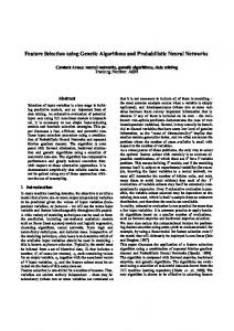
consider a marginal histogram, the total size of all the bins should be H × n. Figure 1 shows an example of marginal FWH on variable xj. The bin width ε can be determined by choosing appropriate number of bins depending on the required precision for a given problem. For multimodal problems, we need consider some maximum bound onε value. Let us consider the worst case scenario where the peak with the global optimum of h1 has smaller width w1 than ε and the second best local optimum has a much wider peak of width w2 (Figure 2). Moreover, let us assume that all solutions in each peak are very close to the peak p jHWH ( as it should be the case later in the run). In this case, after the random sampling at generation 0, the mean fitness of individuals in the bin where the second best solution is located is h 2 and mean fitness of individuals in the bin where the best solution is located is h 1 × w 1 /(2 ε ). With most selection schemes, if h2 >h1 × w1/(2ε) holds, then max min xj the probability density of the bin where the second best solution is located increases more than the Figure 1: Marginal fixed-width histogram (FWH) probability density of bin where the best solution is located. As a result, the algorithm converges to the f(x) second best optimum instead of the global one. To best solution w1 h1 prevent this, the following relationship must hold: second best solution w1 × h1 ε< h2 . (2) 2 × h2 2.2.2 Sampling methods In the FWH, new individuals are generated as follows: first a bin is selected according to the probability ε given by Eq. (1). Then an individual is generated by generating a number from the bin with uniform Figure 2 Fitness function with multimodality distribution. This is repeated until all individuals are obtained. The simplest method to sample each bin is to use a roulette wheel (RW). However, RW has a certain amount of stochastic sampling error. Let S be the total number of samples. Then the distribution of R, the number of samples from bin hj , is R S −R S j j PShj ( R ) = × PFWH [ h] 1 − PFWH [h ] , R = 0,1,..., S (3) R and the expected value of R is
(
)(
)
j R = S × PFWH [h ] . Let us define a "normalized number of samples" r = R/S, then distribution of r is obtained as
(4)
PShj ( r ) = S × PShj ( R / S ), r = [0, 1] . Figure 3 shows an example of distribution r for various number of S. 9 FjFWH[h] = 0.1 is assumed. Then the expected value of r should be 8
(5)
r = R/S
j = S × PFWH [ h] / S
7
(6)
6
S=10 S=20 S=30
PShj (r ) 5 = 0.1. S=40 4 In Figure 3, we can make sure the existence of the stochastic 3 sampling error, although as S becomes larger, the probability hj density PS (r ) around r = 0.1 increases. 2 One well known sampling method to reduce this sampling error 1 is Baker's stochastic universal sampling (SUS), which was proposed 0 0.0 0.1 0.2 0.3 0.4 0.5 0.6 0.7 0.8 0.9 1.0 for proportional selection operator [1]. In this method, the integer r part of the expected number R is deteministically sampled and the Figure 3: An example of distribution H fraction part of R is stochastically sampled without duplicate. We for various values of 5
KES' 01 N. Baba et al. (Eds.) IOS Press, 2001
115
extend this method to sample from marginal histogram models. We call this method E-SUS (extended SUS). A pseudo C code of E-SUS for FWH is described in Figure 4. To apply this method, The variable "expected" in line 13 is the expected sampling number for bin h of variable xj. For instance, if the probability of a particular bin is 0.155 and we want to sample 100 individuals, we would expect 15.5 copies of representatives of the bin. The presented algorithm will generate 15 copies and then another copy with probability 0.5. To obtain a random combination among variables, we must shuffle the sampling sequence for each dimension (line 8). In the experiments in Section 3, we use both the RW and the E-SUS.
2.3 Marginal fixed-height histogram (FHH) 2.3.1 Model description
1 // S: sampling individual number, n: number of variables, H: number of bins 2 // p[j][h]: probability density of bin h of variable x j 3 // [j][h]: left edge position of of bin h of variable x j 4 // Rand(): generate random number from [0, 1.0] 5 V[S][n]; // array for sampled vectors 6 xh[S]={0,1,2,……S-1}; // array for random permutation of bin position 7 for(int j=0; j