Nonlocal processing of 3D colored point clouds - Hal

Nonlocal processing of 3D colored point clouds Fran¸cois Lozes, Abderrahim Elmoataz, Olivier L´ezoray

To cite this version: Fran¸cois Lozes, Abderrahim Elmoataz, Olivier L´ezoray. Nonlocal processing of 3D colored point clouds. International Conference on Pattern Recognition, 2012, Tsukuba, Japan. pp.1968-1971, 2012.

HAL Id: hal-01108865 https://hal.archives-ouvertes.fr/hal-01108865 Submitted on 31 Mar 2015

HAL is a multi-disciplinary open access archive for the deposit and dissemination of scientific research documents, whether they are published or not. The documents may come from teaching and research institutions in France or abroad, or from public or private research centers.

L’archive ouverte pluridisciplinaire HAL, est destin´ee au d´epˆot et `a la diffusion de documents scientifiques de niveau recherche, publi´es ou non, ´emanant des ´etablissements d’enseignement et de recherche fran¸cais ou ´etrangers, des laboratoires publics ou priv´es.

Nonlocal processing of 3D colored point clouds Franc¸ois Lozes, Abderrahim Elmoataz, Olivier L´ezoray Universit´e de Caen Basse-Normandie,GREYC UMR CNRS 6072 ENSICAEN - Image Team, 6 Bd. Mar´echal Juin, F-14050 Caen, France. {francois.lozes,abderrahim.elmoataz-billah,olivier.lezoray}@unicaen.fr

Abstract In this paper we present a methodology for nonlocal processing of 3D colored point clouds using regularization of functions defined on weighted graphs. To adapt it to nonlocal processing of 3D data, a new definition of patches for 3D point clouds is introduced and used for nonlocal filtering of 3D data such as colored point clouds. Results illustrate the benefits of our non-local approach to filter noisy 3D colored point clouds (either on spatial or colorimetric information).

1. Introduction With the advent of nonlocal processing of images [2], patch-based approaches have been recently very popular. However, the notion of patches is difficult to extend to 3D point clouds. Indeed, for images, the notion of patch relies on the spatial organization of pixels in a grid. With point clouds, the data to process is not organized on any Cartesian grid and the neighbors of a point have to be defined. Even with such neighbors defined (e.g., by creating a graph), one has no insurance that the number of neighbors of two different points will be the same and this makes difficult the comparison of these two neighborhoods. Therefore, there is actually no natural expression of what is a patch on a point cloud. Recently, some authors have experimented nonlocal denoising point clouds [6]. However this approach does not take into account any orientation information of the patch and is used only to denoise spatial information and not any spectral information attached to the points. In this paper, we propose an approach relying on the framework of Partial difference Equations (PdEs) to perform graph regularization [3] in order to filter 3D colored point clouds. To do so we introduce an innovative way to define patches for 3D points clouds in order to perform nonlocal processing.

2. Weighted Graphs In this section, we recall definitions on graphs and operators on graphs. This constitutes the basis of the framework of PdEs to regularize a function on a graph.

2.1

Definitions

A weighted graph G = (V, E, w) consists in a finite set V = {v1 , . . . , vN } of N vertices and a finite set E ⊂ V × V of weighted edges. We assume G to be undirected, with no self-loops and no multiple edges. Let (u, v) be the edge of E that connects vertices u and v of V. Its weight, denoted by w(u, v), represents the similarity between its vertices. Similarities are usually computed by using a positive symmetric function w : V × V → R+ satisfying w(u, v) = 0 if (u, v) ∈ / E. The notation u ∼ v is also used to denote two adjacent vertices. Let H(V) be the Hilbert space of real-valued functions defined on the vertices of a graph. A function f : V → R of H(V) assigns a real value f (vi ) to each vertex vi ∈ V. The space H(V) isP endowed with the usual inner product hf, hiH(V) = u∈V f (u)h(u), where f, h : V → R. Similarly, one can define H(E), the space of real-valued functions defined on the edges of G.

2.2

Difference operators on weighted graphs

Let G = (V, E, w) be a weighted graph, and let f : V → R be a function of H(V). The difference operator [3] of f , noted dw : H(V) → H(E), is defined p on an edge (vi , vj ) ∈ E by: (dw f )(vi , vj ) = w(vi , vj )(f (vj ) − f (vi )). The directional derivative (or edge derivative of f , at a vertex vi ∈ V, along an edge e = (vi , vj ), is defined as: ∂vj f (vi ) = (dw f )(vi , vj ). The adjoint of the difference operator, noted d∗w : H(E) → H(V), is a linear operator defined by: hdw f, HiH(E) = hf, d∗w HiH(V) for all f ∈ H(V) and all H ∈ H(E).

∗ ∗ We obtain p the expression of dw by: (dw H)(vi ) = P w(vi , vj )(H(vj , vi ) − H(vi , vj )). The divj ∼vi vergence operator, defined by −d∗w , measures the net outflow of a function of H(E) at each vertex of the graph. The weighted gradient operator of a function f ∈ H(V), at a vertex vi ∈ V, is the vector operator defined by: (∇w f)(vi ) = [∂vj f (vi ) : vj ∼ vi ]T , ∀(vi , vj ) ∈ E. The L2 norm of this vector represents the local variation of the function f at a vertex of the graph. It is defined by [3]: k(∇w f)(vi )kp = hP p i1/p w(vi , vj )p/2 f (vj )−f (vi ) . v∼vi

2.3

Nonlocal regularization on graphs

In this section, one considers a general function f 0 : V ⊂ Rn → Rm defined on graphs of the arbitrary topologies and we want to regularize this function. The regularization of such a function corresponds to an optimization problem that can be formalized by the minimization P of an energy as a weighted sum of two energy terms: 12 vi ∈V ||∇w f(vi )||22 + λ2 kf − f 0 k22 The first term is the regularization term, meanwhile the second is the fitting term. The parameter λ ≥ 0 is a fidelity parameter that specifies the trade-off between the two competing terms. Works of [3] have shown that solutions minimizing such an energy on weighted graphs can be obtained by the following iterative algorithm ∀u ∈ V:   

f (0) (vi ) = f 0 (vi )

P λf 0 (vi ) + v∼vi w(vi , vj )f (n) (vj ) P λ + vj ∼vi w(vi , vj ) (1) Equation (1) describes a family of discrete diffusion processes, which is parameterized by the structure of the graph (topology and weight function w), the parameter λ. As shown in [3], modifying both graph topology and graph weights enables to perform both local and nonlocal filtering within the same framework of PdEs. This iterative algorithm stops when a number of iterations is reached, or when the difference ||f n+1 − f n || is small. (n+1)  (vi ) = f

properties of the point cloud. We review the principle of our approach that relies on four steps.

3.1

Graph creation from 3D point clouds

Let us consider a point cloud P as a set of data points {p1 , . . . , pn } ∈ R3 . There are many ways of associating a graph, that encodes proximity between points, to such a data set. To each data point we first associate a vertex of a proximity graph G to define a set of vertices V = {v1 , v2 , . . . , vn }. Then, determining the edge set E of the proximity graph G requires defining the neighbors of each vertex vi according to its embedding pi using the Euclidean distance. We will denote as D(vi , vj ) = kpi − pj k2 the Euclidean distance between vertices and as B(vi ; r) = {pj ∈ Rn | D(vi , vj ) ≤ r} the closed ball of radius r centered on pi . We consider two types of graphs: i) the -ball graph: vi ∼ vj if pj ∈ B(vi ; ), ii) The k nearest neighbor graph (kNNG): vi ∼ vj if the distance between pi and pi is among the k-th smallest distances from xi to other data points. The first step consists in associating a k-NNG graph to the 3D point cloud.

3.2

Tangent plane estimation

Second step consists in computing an approximation of the tangent plane of a point pi (or the vertex vi ). Classically (see [5]), the PCA of the covariance matrix of the neighbors of vi in a local -ball graph around vi is considered. Let p(vi ) be the centroid of the neighbors of vi . The covariance matrix of the local    T frame is C = pj − p(vi ) · pj − p(vi ) with vj ∼ vi . From this matrix, eigenvalues λ0 < λ1 < λ2 and eigenvectors t0 (vi ), t1 (vi ), t2 (vi ) are computed. Eigenvectors t1 (vi ) and t2 (vi ) form an orthogonal basis of the tangent plane, and t0 (vi ) is normal to this tangent plane (Figure 1).

3. Processing of 3D point clouds In contrast to existing works, we propose to make the most of weighted graphs to define the notion of patches for 3D colored point clouds. In addition to providing an innovative definition of patches for 3D point clouds, our approach can be used to denoise spatial or/and spectral

Figure 1: Estimation of the tangent plane for a given point pi according to a set of neighbors. The centroid the set of neighbors of pi in B(vi ; r) is p(vi ). Computed tangent vectors are t1 (vi ) and t2 (vi ).

3.3

Orientation estimation

Third step consists in estimating orientations. Indeed, patches are oriented from principal directions. This means that directions of first and second axis of the patch basis will coincide respectively with major and minor principal directions. To compute these principal directions at point pi , we use the arguments of [1]. Principal directions and principal curvatures can be estimated from the PCA of the covariance matrix of the normals of the neighbors of pi projected on the tangent plane of pi . Let n(vj ) be the normal associated to node vj (this is estimated [4] from the tangent plane normal as ±t0 (vi )  T ) and ξ(vj ) = n(vj ) · t1 (vi ); n(vj ) · t2 (vi ) be the projection of the normal n(vj ) on the tangent plane (t1 (vi ), t2 (vi )). Then the covariance matrix Cn of these projected normals of all the neighbors of a given point (in the local epsilon-ball graph) is computed as   T  Cn = ξ(vj ) − ξ(vi ) · ξ(vj ) − ξ(vi ) with vj ∼ vi and ξ(vi ) the centroid of the projected normals. From this matrix, eigenvalues λ0 < λ1 and eigenvectors c0 (vi ), c1 (vi ) are computed. Then, c0 (vi ), c1 (vi ) are respectively estimations of the minor and major principal directions.

3.4

Patch construction

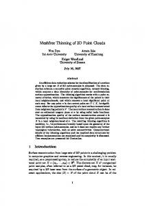
Final step consists in constructing the patches. Given a point pi , defining a patch for this point comes to construct a square grid around pi on its tangent plane. We fix the patch length as l = 2 × maxvj ∼vi kpj − pi k. A square lattice of n2 cells is then constructed around pi with respect to the basis obtained from principal directions c0 (vi ), c1 (vi ). Each cell has a side length of l/n. Then, all the neighbors vj of vi are projected on the tangent plane of pi giving rise to projected points p0j . To fill the patch with values, these projected points p0j are affected to the cells the center of which is the closest. The value of the cell is then deduced from the average of the values f 0 (vj ) associated to the vertices vj that where affected to the patch cell. This value can be a spatial value (the projected points’ coordinates) or a spectral one (the points’ colors). The set of values inside the patch of the vertex vi are denoted as P(vi ). Figure 2 summarizes the method.

4. Experiments The proposed framework is used to denoise coordinates of noisy 3D point clouds and to filter colored point clouds. Let f 0 : V → R3 be the function

Figure 2: Interpolation of the content of the patch. l is the patch length. c0 (vi ) and c1 (vi ) are the principal directions at a point pi . Elements marked by a “+” symbol correspond to the projected neighbors of pi on the patch. These projections are used to deduce values of each patch cell. that associates either 3D coordinates or RGB colors to each node u ∈ V. From this function, a graph G(V, E, w) is first created. We consider 10 nearest neighbor graphs for all the experiments with 10 iterations of algorithm (1). The graph is weighted with ||F(f 0 ,vi )−F(f 0 ,vj )||2 ). If ones conw(vi , vj ) = exp(− σ2 siders local weights, F(f 0 , vi ) = f 0 (vi ). In the case of nonlocal weights (based on patches), one has F(f 0 , vi ) = P(vi ). We first consider the case of 3D point clouds where f 0 (vi ) = pi . Figure 3 presents results on two points clouds corrupted by Gaussian noise and compares the effect of local versus nonlocal regularization. The benefit of our formulation of nonlocal denoising of 3D point clouds is evident with a final point cloud much more close to the shape of the original uncorrupted one. Second we consider the case of 3D colored point clouds where f 0 (vi ) = [Ri , Gi , Bi ]T . Figure 4 presents results of color filtering on a given 3D colored point clouds (obtained from a laser scan of a Maya temple wall). It is important to notice that this point cloud is not a triangular mesh but a raw 3D colored point cloud. As attended, local filtering tends to remove many details while blurring borders. On the opposite, our formulation of nonlocal filtering achieves a much better job while preserving edges and providing uniform zones of similar textures.

5. Conclusion In this paper we proposed a nonlocal processing of 3D colored point clouds. Using nonlocal regularization on graphs to filter point clouds, we demonstrated how to define the notion of patches for point clouds. To define a patch a given point pi , its tangent plane is first determined and its principal directions are estimated. Then, a grid lattice representing the patch is constructed around the point pi and all the neighbors of pi in the graph are

Initial colored point cloud

Local filtering

Non-local filtering

Figure 4: Local and nonlocal (3 × 3 patches) filtering of a 3D colored point cloud acquired by a laser scan of a Maya temple wall. First line present the full point cloud. Second line presents a cropped and zoomed area. projected onto the grid. On this grid, an interpolation is finally used from projected points to fill the patch. Experimental results have shown the benefits of the approach that enables the nonlocal filtering of 3D colored point clouds within a unified formalism. Future works will consider the case of inpainting 3D colored point clouds.

References

Figure 3: Denoising of two noisy 3D point clouds coordinates (in columns). From top to bottom lines: original, corrupted (σ = 20), locally denoised, and nonlocally (3 × 3 patches) denoised point clouds.

[1] J. Berkmann and T. Caelli. Computation of surface geometry and segmentation using covariance techniques. IEEE Trans. Pat. Anal. Mach., 16(11):1114–1116, 1994. [2] A. Buades, B. Coll, and J.-M. Morel. A non-local algorithm for image denoising. In CVPR, pages 60–65, 2005. [3] A. Elmoataz, O. Lezoray, and S. Bougleux. Nonlocal discrete regularization on weighted graphs: a framework for image and manifold processing. IEEE Trans. on Im. Proc., 17(7):1047–1060, 2008. [4] H. Hoppe, T. DeRose, T. Duchamp, J. McDonald, and W. Stuetzle. Surface reconstruction from unorganized points. SIGGRAPH Comput. Graph., 26(2):71–78, 1992. [5] M. Pauly. Point primitives for interactive modeling and processing of 3D geometry. Selected readings in vision and graphics. Hartung-Gorre, 2003. [6] R.-F. Wang, W.-Z. Chen, S.-Y. Zhang, Y. Zhang, and X.Z. Ye. Similarity-based denoising of point-sampled surfaces. J. of Zhejiang. Univ. -Science A, 9(6):807–815, 2008.