Nonparametric Slope Estimators for Fixed-Effect Panel Data

Nonparametric Slope Estimators for Fixed-Effect Panel Data Kusum Mundra1 Department of Economics San Diego State University San Diego, CA 92182 October 2004

1I

would like to acknowledge helpful comments from Aman Ullah. This version also includes many constructive suggestions received from participants at the 11th International Panel Data Conference, in July 2004 at the Texas A&M University.

Abstract There are more data sets being available in panel form, msking panel data estimation techniques very popular in applied econometrics. Dependent on how the sample is drawn from the population, the cross sectional effect is treated as fixed or random. In this paper, I present two nonparanetric slope estimation for fixed effect panel models. It is will known in theoretical econometrics that misspecification of the functional form leads to biased estimates of the parameters. In particular, there has been extensive work on semiparametric or more appropriately partially linear models, however the literature does not talk enough on nonparametric panel models. Recently there has been some work in the nonparametric estimation of random effect models, see Henderson and Ullah (2003). Unfortunately the literature does not talk about nonparametric fixed-effect slope estimation, in this paper I intent to fill that gap. Two nonparametric slope estimates for fixed effect panel models are discussed with the asymptotics established. Finite sample Monte Carlo properties are discussed. I apply the nonparametric estimators to investigate the effect of age and tenure on the workers hourly wages using NLSY79 (National Longitudinal Survey of Youth Data). In estimating earning functions it is a very common practice to assume workers earnings being quadratic in age and tenure, the estimation shows that the parametric slope shows a steady decline in hourly earnings as age goes up but the nonparametric slope shows that the decline is not steady. In addition, the nonparametric estimator shows that for bigger magnitude of tenure the effect on the hourly wages is quite different from the lower weeks of tenure.

1

Introduction

More data sets are being available in panel form, making panel data estimation techniques very popular in applied econometrics. In panel data we are able to get observations over cross-sectional units over time and we can capture the cross-ssectional heterogeneity by including an individual or cross-sectional effect in our model. Dependent on how the sample is drawn, the cross sectional effect is treated as fixed or random.

In the random effect specification it is assumed that the cross section is

drawn from a random population and the cross sectional effect is part of the stochastic error. Whereas in the fixed effect model, the cross sectional effect capturing the cross-section heterogeneity is not a part of the error but it is a parameter varying across the cross-section. The cross sectional effect when treated as fixed and nonrandom, allows the cross sectional effect for the cross section i to be correlated with other exogenous regressors in the model. 1 In this paper, we present two nonparanetric slope estimation for fixed effect panel models. It is will known in theoretical econometrics that misspecification of the functional form leads to biased estimates of the parameters. and often policies are based on these biased estimates, making this a significant problem in applied econometrics. The significance of functional form in the modelling makes nonparametric analysis very important. In nonparametric models, no specific functional form is imposed on how does the indepenedent variable affects the dependent variable, see Ullah and Pagan (1999). An important extension of nonparametric Kernel techniques have been to panel data models, see Ullah and Roy (1998), Porter (1996). In particular, there has been extensive work on semiparametric or more appropriately partially linear models (where some dependent variable in the regression model enter linearly and for others the functional form is not known, and hence partially linear), see Li and Stengos (1996), Li and Ullah (1998) and Berg, Li and Ullah (2000). However, there has not been enough work on nonparametric panel models, recently there has been some work in the nonparametric estimation of random effect models, see Henderson (2004). Unfortunately the literature does not talk about nonparametric fixed-effect slope estimation, in this paper we intent to fill that gap. This paper presents two 1

For discussion on different panel data estimation and treatment of the cross-sectional effect see Hsiao (2003 ), Baltagi (2002) and Mundlak (1978).

1

nonparametric slope estimates for fixed effect panel model. The estimators are applied to estimate earning functions using NLSY data. This paper is organized as follows. Section 2 specifies the model and gives the estimates and section 3 establishes the asymptotics of the estimates. Monte Carlo results are discussed in section 4. Section 5 presents the application of the two estimates to earning function using NLSY data. Finally, section 6 concludes.

2

Nonparametric Slope Estimation

The parametric (linear) fixed-effcet panel model is specified as follows: yit = αi + zit β + uit

i = 1, ..., n t = 1, ..., T

(2.1)

where yit is the dependent variable, zit is a matrix of k exogenous variable and β is a k × 1 vector and αi is the cross-sectional effect that is treated as non-random and

is a fixed unknown parameter to be estimated. The error uit is assumed to follows the usual iid error structure with mean zero and constant variance. The nonparametric model given in (2.1) with the fixed effect is as follows yit = αi + m(zit ) + uit

i = 1, ..., n t = 1, ..., T

(2.2)

where we do not specify how zit effects yit, the unknown functional form m(.) makes the model a nonparametric model. The problem is to estimate β (the parametric slope) in the model (2.1) nonparametrically in (2.2). The nonparametric approach is to use the nonparametric kernel regression estimation of the unknown form m(zit ) and estimate m0 (zit ), where m0 (zit ) is the first derivative of m(zit ) with respect to zit . The model in (2.2) can be written as yit = αi + m(z) + (zit − z)β(z) + (1/2)(zit − z)2 m2 (z) + uit

(2.3)

where we expand the unknown regression around a point z, to the third order, the idea being in (2.3) to estimate the slope m0 (zit ) in (2.2) locally in the interval h around z by linear approximation (zit − z)β(z).2 2

This is similar to the nonparametric kernel regression functional, varying coefficient models proposed by Lee and Ullah ( 2003), Cai et al. (2000).

2

There are two well known transformations used to take care of the fixed effect in the parametric models, one is first differencing yit − yit−1 and the second is takP ing deviations from mean yit − y¯i. = yit − T1 yit , see Hsiao (2003), Baltagi (2002), Chamberlain (1984), Matyas and Sevestre (1996). In the linear parametric panel model little is known how these two methods compare against each other, in section 4 of this paper I present some Monte Carlo simulations results for the two transformations. In this paper, we use the two transformations to the fixed effect nonparametric panel data models and estimate the slope coefficients with local linear kernel weighted techniques. In the first estimator, we use the first differencing transformation to take account of the cross-sectional effect while estimatig the slope parameter of interest. In the second estimator deviation from mean is used.

2.1

First - Differencing Estimator

After taking a first difference of (2.3) we get:

1 ∆yit = (zit − zit−1 )β(z) + [(zit − z)2 − (zit−1 − z)2 ]m2 (z) + ∆uit + r 2

(2.4)

where β(z) = m1 (z) is the slope parameter of interest and r is the remainder term. The model is (2.4) can also be written as A2 Y ˜A2 Zβ(z) + A2 U  −1 1 0 . . . 0  0 −1 1 . . . 0   matrix of order n(T-1) x nT. where A2 is   . . . . . . .  0 0 . . . −1 1 The local linear estimator of is the parameter of interest and is given by, 

ˆ β(z) = (Z 0 A2 KA2 Z)−1 Z 0 A2 KA2 Y

(2.5)

or ˆ β(z) =

T n X X wit ∆yit i=1 t=2

3

(2.6)

∆zit Kit Kit−1 , see Pagan and Ullah (1999). Where Kit = K( zith−z ) ΣΣ∆2 zit Kit Kit−1 −z K( zit−1 ) are the standard normal kernel function with optimal window h

where wit = and Kit−1 = width h.3 .

2.2

Deviation from Mean Estimator

Deviation from mean transformation for the panel data model is proposed as follows4 :

where y¯i. =

1 T

from (2.1) gives

y¯i. = αi + m(z) + (¯ zi. − z)β(z) + ui. + r (2.7) P P P yit , z¯i. = T1 zit , and ui. = T1 uit . Taking a difference of (2.7) yit − y¯i. = (zit − z¯i. )β(z) + uit − ui. + r

The local FE estimator of the slope β(z) can then be obtained by minimizing ΣΣ(yit − y¯i. − (zit − z¯i. )β(z))2 K( zith−z ).This gives, for q = 1,the slope estimator as i t

follows:

˜ β(z) =

XX Kit (yit − y¯i. )(zit − z¯i. ) i

and for q ≥ 1,

t

ΣΣKit (zit − z¯i. )2

,

(2.8)

i t

˜ β(z) = (X 0 MD K(z)MD X)−1 X 0 MD K(z)MD y ¯T , Q ¯T = where MD = INT − D(D0 D)−1 D0 = INT ⊗ QT and QT = IT − Q

3

ιT ι0T T

Asymptotic Properties of the Estimators

In this section asymptotic properties of the estimators are established and asymptotic distributions of the above estimators are derived. The assumptions and steps are similar to those of Robinson (1986, 1988a, 1988b), Kneisner and Li (2002) 3 See Pagan and Ullah (1999) for well established properties of the standard normal kernel and details on the optimal window width (bandwidth) selection. 4 In Ullah and Roy (1997) the mean deviation nonparametric fixed effect estimator was mentioned but the properties of the estimator were not discussed.

4

Following Robinson (1988) let Gλµ denote the class of functions such that if g ² Gλµ , then g is µ times differentiable; g and its derivatives (up to order µ) are all bounded by some function that has λ − th order finite moments. Also, K2 denotes the class of R non-negative kernel functions k : satisfying k(v) v m dv = δom for m = 0 , 1(δom is R the Kronecker’s delta), k(v)vv0 dv = Ck I(I > 0 , and k(u) = O((1+ | u |3+η )−1 ) for R some η > 0. Further, k 2 (v)vv0 dv = Dk .I. Property 1: Under the following assumptions (1) (i) for all t,

(yit , zit ) are i.i.d. across i.zit is a strictly stationary real valued

stochastic process and zit and zit−1 admits a joint density function f ² G∞ µ−1 . m(zit ) and m(zit−1 ) both ² G4µ−1 for some positive integer µ > 2. uit ,

(2) E(uit | zit , zit−1 ) = 0 , E(u2it | zit , zit−1 ) = σ 2 is continuous in zit and zit , and (3) k ² K2 and k(v) ≥ 0 ; as n → ∞ , h → 0 , nhq+3 → ∞ and nhq+4 → 0. ³ ´ √ ˆ nT hq+3 β(z) − β(z) ˜N (0, Σ)

for large N and fixed T, where R ' m2 (z) (µ2 f(z, z)) h−1, Φ = 4σ 2 µ2 f (z, z) (µ2 − 1) ,

Σ = R−1 ΦR−1

For the derivation of the property 1 see Appendix A. Property 2: Under the following assumptions (1) (i) for all t,

(yit , zit ) are i.i.d. across i and zit admits a density function

4 f ² G∞ µ−1 , m(zit ) ² Gµ−1 for some positive integer µ > 2.

(2) E(uit |zit ) = 0 , E(u2it | zit ) = σ 2u is continuous in zit , and uit ,

(3) K ² K2 and k(v) ≥ 0 ; as n → ∞ , h → 0 , nhq+2 → ∞ and nhq+3 → 0. ³ ´ √ ˜ − β(z) ˜N (0, Σ1 ) nT hq+2 β(z)

where Σ1 = R1−1 Φ1 R−1 , where R1 = T 2 z 2 f(z) and Φ1 = For the derivation of the property 2 see, Appendix B.

5

(T −1) 2 R σu[ T

K 2 (ψ 1t ) ψ 21t dψ 1t ].

4

Monte Carlo Results

In this section we discuss the Monte Carlo properties of the above estimators for different sizes of sample, to investigate the finite sample properties.5 Firstly, the monte carlo properties is investigated and compared between the two prametric linear fixed effect models.

Secondly in this section, we present the above nonparametric

fixed effect estimators. For the parametric linear model the following data generating process is used is yit = αi + zit β + uit

(4.1)

where αi is the cross sectional fixed effect and is generated by αi = 2.5 + αj , this allows that the fixed effect for unit i is correlated with j. The above model (where the data generation is linear) is estimated by both the methods, deviation from´mean P ³b b −1 and first differencing for different N and T. The Bias(β) = M β − β and j

b = RMSE(β)

(

´2 P ³b M −1 βj − β j

)−1/2

j

, where M is the number of replications, β j

is the estimate of β at the j − th replication using NT observations. M = 2000 in the

parametric simulation and T is varied to be 3, 6, 10, 50,100, and 500. While N takes the values 10, 50, 100, 500, and 1000. The parametric estimators are as follows: (1) Parametric first differencing estimator PP (z − z ) (y − y ) b PitP it−1 it 2 it−1 β dif f = (zit − zit−1 )

(2) Parametric mena deviation estimator PP (zit − z i. ) (yit − y i. ) bdev = β PP (zit − z i. )2

Following the methodology of Baltagi, Chang and Li (1992 ), Li and Ullah (1992) xit is generated by the process used by Nerlove (1971), where zit = o.1t+0.5zit−1 +wit , where zio = 10 + 5wio and wit ∼ U [−0.5, 0.5], uit is drawn from standard normal distribution and β is chosen to be 8. The simulation results showing the difference

between the RMSE of the two parametric slope estimators are given in Table 1 (Panel 5

This Section is work in progress.

6

A). In another exercise the data is generated by the method followed in Berg, Li √ √ and Ullah (.) where zit ∼ U [− 3, 3], the results are given in Table 1 (Panel B).

From Table 1 (both Panel A and Panel B) we see that for all N as T increases

first differencing fixed effect slope estimator for linear model is doing better than the mean-deviation estimator. We see that the difference between the root mean square of the first-differencing and the mean deviation estimator is steadily rising as T goes up. The bias and the standard error for the first differencing etsimator is lower than the mean-deviation etsimator as T increases for all N. For the nonparametric model the following data generating process is used is yit = αi + zit β 1 + zit2 β 2 + uit

(4.2)

where zit ∼ U [−0.5, 0.5] by Berg. Li and Ullah method and αi is generated by

αi = vi + c2 αj , where vi ˜N (0, σ v ), M = 1000 for the nonparametric simulations. The value of β 1 is chosen to be 0.5, β 2 is chosen to be 2, and c1 is chosen to be 2. The value of σ 2v + σ 2u = 20 and ρ = σ 2u /(σ 2v + σ 2u ) takes the value of 0.8. In the above model the true data generation is quadratic and the model is estimated by both the nonparametric methods proposed in the previous sections; deviation from mean and first differencing. T is varied to be 3,6,10, while N takes the values 10, 50, 100. For comparison purposes we also compute the parametric fixed effect slope estimator for bdif f ) and the mean deviation (β bdev ) the model given in (4.2 ) by the differencing (β

estimator. Both in the case of the differencing transformation (Table 2) and in the case of the mean deviation transformation (Table 3) compared to the parametric estimators nonparametric estimator is doing better ∀ N and T. Also, we see that for

fixed T and increasing N in both the estimators the difference in the RM SE is falling between the parametric and the nonparametric etsimators. Treating the cross sectional effect as the fixed effect allows that the individual effect maybe correlated with one or more of the explanatory variables (is very common when the model is misspecified, Hsiao (2003). In order to investigate the difference between the RMSE for the nonparametric and the parametric etsimator we carry out the above monte carlo simulation αi to be correlated with z i. by αi = vi + c1 z i. + c2 αj , where the value of c1 = 2 and c2 = 2, results from the simulation are given in Table 4 and Table 5. Compared to the cases where αi is not correlated with z i. , we see that the difference between the RM SE of the parametric and the nonparametric estimator 7

has gone up when we allow the fixed effect to be correlated with the explanatory variable. We also incraese the degree of nonlinearity in the model given by (4.2), by increasing the value of β 2 from 2 to 4 and αi = vi + c2 αj , where c2 = 2. From Table 6 and Table 7 we see that in small samples the nonparametric estimator is doing better.

5

Application

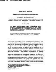
In this part, we apply the nonparametric mean deviation estimator to investigate the effect of age and tenure on the workers hourly wages using NLSY79 (National Longitudinal Survey of Youth Data). This a well known panel data that uses surveys by the Bureau of Labor Statistics (BLS) to gather information on the labor market experiences of diverse groups of men and women in the U.S. at different tim points.6 In estimating earning functions it is a very common practice to assume workers earnings being quadratic in age and tenure, see Angrist and Krueger (1991), Sander (1992), Vella and Verbeek (1998) and Rivera-Batiz (1999) to name a few. Using the fixed effect mean-deviation estimator the earnings slope is estimated with respect to age and tenure uisng a sample of 1000 individuals for t = 3 (the years are 1994, 1996, and 1998). For the parametric model the earning function is assumed to be quadratic in age (measured in years) and tenure (measured in weeks). The slope estimates are presented for age in Figure 1 and for tenure in Figure 2, respectively. Figure 1 shows that for all the individuals in the sample the parametric slope (shows a steady decline in hourly earnings as age goes up but the nonparametric slope shows that the decline is not steady. Also, the magnitude of the parametric results is very high compared to the nonparametric results. The parametric effect of tenure on wage shows that an additional gain of a week has close to zero effect on the hourly earnings. The nonparametric estimator shows that for bigger magnitude of tenure the effect on the hourly wages is quite different from the lower weeks of tenure. 6

The NLS contractors for the BLS are the Centre for Human Resource Research (CHRR) at the Ohio State University, The National Opinion Research Center at the University of Chicago, and the U.S. Census Bureau.

8

Figure 3 and Figure 4 shows the nonparametric slope for age and tenure respectively through first-differencing transformation.

6

Appendix

6.1

Proof of Theorem 1

T n P P ˆ For q = 1 as β(z) = (Z 0 A2 KA2 Z)−1 Z 0 A2 KA2 Y = wit ∆yit i=1t=2

where wit =

∆zit Kit Kit−1 . ΣΣ∆2 zit Kit Kit−1

Refer to (2.5). This proof is for q = 1, but can easily

be generalized. PP ˆ Write, E(β(z)/z wit (m(zit ) − m(zit−1 ))) it , zit−1 ) = E( ˆ . Approximated £ / zit , zit−1 ) ¤ 2 µ µvalue is E(β(z) ¶¶ 2 PP ∆zit β(z)£+ 12 (zit − z)2 − (zit−1 − z) m (z) ¤ ˜E wit . + 16 (zit − z)3 − (zit−1 − z)3 m3 (z) PP Using ∆zit wit = 1 ˆ the approximated bias is, E(β(z)/z it , zit−1 ) − β(z) = ¡1 £ ¤ £ ¤¢ E 2 wit m2 (z) (zit − z)2 − (zit−1 − z)2 + 16 m3 (z)wit (zit − z)3 − (zit−1 − z)3 Using ψ it =

zit −z , h

1

we derive some lemmas.

2

E(D ) = E[ΣΣ∆ zit Kit Kit−1 ] == nT i t

˜nT h4 2µ2 f (z, z) + O(h6 )

ZZ

∆2 zit Kit Kit−1 f (zit , zit−1 )dzit dzit−1

E(D2 ) = E[ΣΣ(zit − z)2 ∆zit Kit Kit−1 ] (A.2) Z Z = = nT h4 (ψ it )2 K (ψ it ) K(ψ it−1 )f (ψ it h + z, ψ it−1 h + z)dψ it dψ it−1 £ ¤ ˜nT −h5 µ2 f (z, z) + h6 µ4 f10 (z, z) − h6 (µ2 )2 f01 (z, z) + O(h7 ) E(D3 ) = E[ΣΣ(zit−1 − z)2 ∆zit Kit Kit−1 ] (A.3) Z Z = = nT h4 (ψ it−1 )2 K (ψ it ) K(ψ it−1 )f (ψ it h + z, ψ it−1 h + z)dψ it dψ it−1 £ ¤ ˜nT h5 f (z, z)µ2 − h6 µ4 f01 (z, z) + 2h6 (µ2 )2 f10 (z, z) + O(h7 ) 9

E(D4 ) = E[ΣΣ∆zit ∆uit Kit Kit−1 ] == 0 i t

where the notation f10 [x, y] represents the partial derivative of f (x, y) with respect to the first variable and f01 [x, y] represents the partial derivative of f (x, y) with respect to the second variable, and f (z, z) is the value of f (x, y) evaluated at x = z, y = z. 1 2 ˆ Combining (A.1-A.3) the approximate bias is: E(β(z)/z it , zit−1 )−β(z) = − 2 m (z)h+

O(h6 ).

Since approximate bias is free from zit , zit−1 it is also approximate unconditional bias. # £ ¤ ∆zit Kit Kit−1 (zit − z)2 − (zit−1 − z)2 + ∆uit ΣΣ∆2 zit Kit Kit−1 XX m2 (z) £ 1 ¤− X X D = { ∆zit Kit Kit−1 (zit − z)2 − ∆zit Kit Kit−1 (zit−1 − z)2 2 XX ∆zit Kit Kit−1 ∆uit }

m2 (z) ˆ β(z) − β(z) = 2

=

"P P

¤ m2 (z) £ 1 ¤−1 £ 2 D D + D 3 + D4 2

Now ³ using ´ lemmas A.1-A.4: D1 E NT h4 = 2µ2 f (z, z) + o(1), thus

m2 (z) E 2

h

D1 NT h4

i−1

→ m2 (z) (µ2 f(z, z))−1 +

o(1) = ³ R.2 ´ ³ 3 ´ D E NT h4 = O (h) = o(1) and E NDT h4 = O (h) = o(1). PP 4 2 ) = E (∆2 zit ∆2 uit K 2 (zit ) K 2 (zit−1 )) = NT h4 4σ 2 f(z, z) (µ2 − 1)+ Also, E(D ³ 4 ´2 2 (z,z)(µ −1) D 2 O(h5 ). E NT = 4σ f(N + O(h5 ). h4 T h4 ) ³ 4 ´ √ Thus NT h4 var NDT h4 = Φ + o(1), where Φ = 4σ 2 f (z, z) (µ2 − 1) . ³ 4 ´ √ d D 4 By Lindberg-Levy Central Limit theorem N T h NT → N (0, Φ) h4 ³ ´ √ ˆ − β(z) ˜N (0, Σ) , where Σ = R−1 ΦR−1 Thus it is proved that NT h4 β(z)

7

Appendix B

˜ For asymptotic normality of β(z) 10

zi. − z)2 + (uit − ui. ] ΣΣKit (zit − z¯i. ) [(zit − z)2 − (¯ 2 m (z) i t ˜ β(z) − β(z) = 2 ΣΣ(zit − z¯i. )2 Kit i t

First I state some lemmas: E(zit2 Kit ≈ hz 2 f (z) + O(h2 )

(B.1)

E(¯ zi.2 Kit ) ≈ hT 2 zf(z) + O(h2 )

(B.2)

E(zit z¯i. Kit ) ≈ hz 2 f(z) + O(h2 )

(B.3)

E(zit3 Kit ) ≈ hz 3 f (z) + O(h2 )

(B.4)

E(zit z¯i.2 Kit ) ≈ hz 3 T 2 f(z) + O(h2 )

(B.5)

E(zit2 z¯i. Kit ) ≈ hz 3 f(z) + O(h2 )

(B.6)

So using (B1-B3) the expectation of the denominator: XX 1 E( (zit − z¯i. )2 Kit ) ≈ T 2 z 2 f (z) + o(1) = R1 NT h t i Similarly using (B1-B6) 1 XX E(Kit (zit − z¯i. ) [(zit − z)2 − (¯ zi. − z)2 ]) ≈ o(1) NT t i

The second moment of µP √ 3 NT h E

P

PP

Kit (zit − z¯i. ) Uit

Kit (zit − z¯i. ) Uit N T h3

¶2

where φ1

≈ φ1 + o(1)

Z (T − 1) 2 = σ u [ K 2 (ψ 1t ) ψ 21t dψ 1t T

By Lindberg-Levy Central Limit theorem 11

(B.7)

Thus,

³X X ´ √ d nT h3 Kit (zit − z¯i. ) Uit → N (0, φ1 ) ³ ´ √ ˜ NT h β(z) − β(z) ˜N (0, Σ1 )

where Σ1 = R1−1 Φ1 R1−1

12

8

References

Angrist, J. D. and A. B. Krueger (1991), Does Compulsory School Attendance Affect Schooling and Earnings? Quarterly Journal of Economics, 106, 979-1014. Baltagi, B. H. (2000), Econometric Analysis of Panel Data, John Wiley, New York. -(1996), Panel Data Methods, forthcoming in, Handbook of Applied Economic Statistics (A. Ullah and D. E. A. Giles, ed.) Marcel Dekker, New York. Baltagi, B. H., Y. J. Chang, and Q. Li (1992), Monte Carlo Results on Several New and Existing Tests for the Error Component Model, Journal of Econometrics, 54, 95-120. Berg, M. D., Q. Li and A. Ullah (1999), Instrumnetal Variable Estimation of Semiparametric Dynamic Panle Data Models: Monte Carlo Results on Several New and Existing Estimators, in Nonstationary Panel, Panel Cointegration and Dynamic Panels (B.H. Baltagi ed.) JAI Press. Cai, Z., J. Fan, and Q. Yao (2000), Functional-Coefficient Regression Models for Nonlinear Time Series, Journal of the American Statistical Association, 88, 298-308. Chamberlain, G. (1984), Panel Data: Handbook of Econometrics (Z. Griliches and M. Intriligator ed.) North-Holland, Amsterdam, 1247-1318. Hsiao, C. (2003), Analysis of Panel Data, Econometric Society Monographs, Cambridge University Press. Kniesner T. and Q. Li, (2002), Nonlinearity in Dynamic Adjustment: Semiparametric Estimation of Panel Labor Supply, Empirical Economics, 27, 131-48. Lee, Tae-Hwy and A. Ullah (2003), Nonparametric Bootstrap Specification Testing in Econometric Models, Computer-Aided Econometrics, Chapter 15, edited by David Giles, Marcel Dekker, New York, pp. 451-477. Li Q. and A. Ullah (1998), Estimating Partially Linear panel Data Models with one-way Error Components Econometric Reviews 17(2):145-166. Li, Q. and T. Stengos (1996), Semiparametric Estimation of Partially Linear Regression Model, Journal of Econometrics 71:389-397. Matyas, L. and P. Sevestre (1996), ed., The Econometrics of Panel Data: A Handbook of the Theory with Applications, Kluwer Academic Publishers, Dordrecht. Mundlak, Y. (1978), On the Pooling of Time Series and Cross-Section Data, 13

Econometrica 46, 69-85. Nerlove, M. (1971), A Note on the Error Components Models, Econometrica, 39, 383-96. Pagan, A. and A. Ullah (1999), Non-Parametric Econometrics, Cambridge University Press. Porter, J. R. (1996), Essays in Econometrics, Ph. D Dissertation, MIT. Rivera-Batiz, F. L. (1999), Undocumented workers in the labor market: An analysis of the earnings of legal and illegal Mexican immigrants in the United States, 12: 91-116. Robinson, P. M.(1986), Nonparametric Methods in Specification, The Economic Journal Supplement, 96, 134-141. (1988a), Root-N Consistent Semiparametric Regression, Econometrica 56:931954. (1988b), Semiparametric econometrics: A Survey, Journal of Applied Econometrics, 3(1), 35-51. Sandler, W. (1992), The Effect of Women’s Schooling on Fertility, Economic Letters, 40, 229-233. Ullah, A. and N. Roy (1998), Parametric and Nonparametric Panel Data Models, in Handbook of Applied Economics and Statistics, edited by A. Ullah and David E. A. Giles, Marcel Dekker. Vella, F. and M. Verbeek (1998), Whose Wages Do Unions Rise? A Dynamic Model of Unionism and Wage Rate Determination for Young Men, Journal of Applied Econometrics 13, 163-183.

14

Table 1: Root Mean Square Error Difference between the two Parametric Slope Estimators 



Panel A: The value in the cell is Rmseβ dev  − Rmseβ diff  for Nerlove data generation N, T

3

6

10

50

100

500

10

1.076 3.866 6.442 10.276 10.507 10.588

50

1.026 3.868 6.439 10.283 10.512 10.590

100

1.036 3.883 6.435 10.285 10.513 10.590

500

1.040 3.876 6.438 10.286 10.512 10.590

1000 1.043 3.879 6.436 10.287 10.513 10.592





Panel B: The value in the cell is Rmseβ dev  − Rmseβ diff  for Berg, Li and Ullah data generation. N, T

3

6

10

50

100

500

10

0.821 1.182 1.682 3.863 5.525 12.773

50

0.350 0.533 0.750 1.742 2.467

5.589

100

0.246 0.370 0.520 1.237 1.765

3.865

500

0.112 0.174 0.225 0.557 0.790

1.763

1000 0.075 0.121 0.166 0.401 0.549

1.816

Table 2: Nonparametric and the Parametric Slope Estimators: First-Differencing b2 = 2, ρ = 0. 8, c1 = 0, c2 = 2 , α i not correlated with z i.  N = 10 T=3  βz  β diff

  Rmseβ diff − Rmseβz

Bias -0.420

Std

T=6 Rmse

Bias

Std

T = 10 Rmse

Bias

Std

Rmse

0.351 0.547 -0.426 0.233 0.485 -0.419 0.164 0.450

-0.0517 2.140 2.139 -0.055 1.406 1.407 -0.011 0.986 0.985 1.592

0.922

0.535

N = 50 T=3  βz  β diff

  Rmseβ diff − Rmseβz

Bias

Std

T=6 Rmse

Bias

Std

T = 10 Rmse

Bias

Std

Rmse

-0.418

0.141 0.441 -0.417 0.103 0.430 -0.411 0.085 0.420

-0.009

0.847 0.847 -0.002 0.619 0.618 0.033 0.508 0.509 0.406

0.189

0.089

N = 100 T=3  βz  β diff

  Rmseβ diff − Rmseβz

Bias

Std

T=6 Rmse

Bias

Std

T = 10 Rmse

Bias

Std

Rmse

-0.422

0.098 0.434 -0.416 0.075 0.423 -0.149 0.057 0.423

-0.032

0.591 0.592 0.003 0.449 0.449 -0.014 0.342 0.343 0.158

0.026

-0.080

Table 3: Nonparametric and the Parametric Slope Estimators: Mean Deviation b2 = 2, ρ = 0. 8, c1 = 0, c2 = 2 , α i not correlated with z i.  N = 10 T=3  βz  β dev

  Rmseβ dev − Rmseβz

Bias

Std

T=6 Rmse

Bias

Std

T = 10 Rmse

Bias

Std

Rmse

0.067 1.842 1.842 0.006 1.267 1.267 0.009 0.948 0.947 0.081 2.417 2.417 -0.001 1.635 1.634 0.013 1.189 1.189 0.575

0.367

0.241

N = 50 T=3  βz  β diff

  Rmseβ dev − Rmseβz

Bias

Std

T=6 Rmse

Bias

0.026 0.796 0.796

-0.01

Std

T = 10 Rmse

Bias

Std

Rmse

0.590 0.590 0.001 0.406 0.405

0.030 1.027 1.026 -0.009 0.745 0.744 0.002 0.517 0.517 0.230

0.154

0.111

N = 100 T=3  βz  β diff

  Rmseβ dev − Rmseβz

Bias

Std

T=6 Rmse

Bias

Std

T = 10 Rmse

Bias

Std

Rmse

0.036 0.566 0.567 -0.008 0.389 0.389 0.015 0.294 0.294 0.037 0.707 0.708 -0.009 0.488 0.487 0.016 0.373 0.373 0.141

0.099

0.079

Table 4: Nonparametric and the Parametric Slope Estimators: First-Differencing b1 = 0. 5,b2 = 2, ρ = 0. 8, c2 = 2, c1 = 2 α i correlated with z i.  N = 10 T=3  βz  β diff

  Rmseβ diff − Rmseβz

Bias

Std

T=6 Rmse

Bias

Std

T = 10 Rmse

Bias

Std

Rmse

-0.421 0.330 0.535 -0.409 0.225 0.467 -0.423 0.170 0.456 -0.022 1.990 1.990 0.048 1.373 1.373 -0.036 1.025 1.025 1.454

0.906

0.569

N = 50 T=3  βz  β diff

  Rmseβ diff − Rmseβz

Bias

Std

T=6 Rmse

Bias

Std

T = 10 Rmse

Bias

Std

Rmse

-0.425 0.140 0.447 -0.420 0.100 0.432 -0.416 0.083 0.424 -0.047 0.839 0.840 -0.020 0.601 0.601 0.007 0.500 0.500 0.392

0.169

0.076

N = 100 T=3  βz  β diff

  Rmseβ diff − Rmseβz

Bias

Std

T=6 Rmse

Bias

Std

T = 10 Rmse

Bias

Std

Rmse

Table 5: Nonparametric and the Parametric Slope Estimators: Mean-Deviation b2 = 2, ρ = 0. 8, c2 = 2, c1 = 2 α i correlated with z i.  N = 10 T=3  βz  β dev

  Rmseβ dev − Rmseβz

Bias

Std

T=6 Rmse

Bias

Std

T = 10 Rmse

Bias

Std

Rmse

0.067 1.842 1.842 0.006 1.267 1.267 0.009 0.948 0.947 0.081 2.417 2.417 -0.001 1.635 1.634 0.013 1.189 1.189 0.575

0.367

0.242

N = 50 T=3  βz  β dev

  Rmseβ dev − Rmseβz

Bias

Std

T=6 Rmse

Bias

Std

T = 10 Rmse

Bias

Std

Rmse

0.049 0.844 0.845 -0.012 0.544 0.544 -0.029 0.426 0.427 0.049 1.068 1.069 -0.013 0.695 0.694 -0.030 0.538 0.539 0.224

0.15

0.112

N = 100 T=3  βz  β diff

  Rmseβ dev − Rmseβz

Bias

Std

T=6 Rmse

Bias

Std

T = 10 Rmse

Bias

Std

Rmse

-0.001 0.568 0.568 -0.008 0.389 0.389 0.000 0.299 0.299 -0.001 0.720 0.720 -0.009 0.488 0.487 0.000 0.388 0.387 0.152

0.098

0.088

Table 6: Nonparametric and the Parametric Slope Estimators with Increased Nonlinearity: First Differencing b2 = 4, ρ = 0. 8, c2 = 2, c1 = 0 α i not correlated with z it  N = 10 T=3  βz  β diff

  Rmseβ diff − Rmseβz

Bias

Std

T=6 Rmse

Bias

Std

T = 10 Rmse

Bias

Std

Rmse

-0.438 0.335 0.551 -0.404 0.236 0.468 -0.421 0.174 0.456 -0.118 2.033 2.036 0.084 1.431 1.433 -0.026 1.046 1.046 1.485

0.965

0.590

N = 50 T=3  βz  β diff

  Rmseβ diff − Rmseβz

Bias

Std

T=6 Rmse

Bias

Std

T = 10 Rmse

Bias

Std

Rmse

-0.414 0.149 0.440 -0.413 0.108 0.427 -0.414 0.082 0.422 0.015 0.897 0.897 0.023 0.650 0.650 0.016 0.491 0.491 0.456

0.223

0.069

N = 100 T=3  βz  β diff

  Rmseβ diff − Rmseβz

Bias

Std

T=6 Rmse

Bias

Std

T = 10 Rmse

Bias

Std

Rmse

-0.417 0.099 0.429 -0.414 0.074 0.420 -0.420 0.060 0.424 -0.002 0.594 0.593 0.018 0.445 0.445 -0.020 0.358 0.359 0.165

0.025

-0.065

Table 7: Nonparametric and the Parametric Slope Estimators with Increased Nonlinearity: Mean-Deviation b2 = 4, ρ = 0. 8, c2 = 2, c1 = 0 α i not correlated with z i.  N = 10 T=3  βz  β dev

  Rmseβ dev − Rmseβz

Bias

Std

T=6 Rmse

Bias

Rmse

Bias

-0.042 1.985 1.985 0.007 1.283 1.282

0.008

0.958 0.957

-0.035 2.578 2.577 0.001 1.654 1.653

0.011

1.202 1.201

0.593

Std

T = 10

0.371

Std

Rmse

0.244

N = 50 T=3  βz  β diff

  Rmseβ dev − Rmseβz

Bias

Std

T=6 Rmse

Bias

Std

T = 10 Rmse

Bias

Std

Rmse

0.028 0.804 0.804 -0.011 0.597 0.596 -0.029 0.405 0.406 0.032 1.037 1.037 -0.010 0.754 0.753 -0.030 0.511 0.512 0.233

0.157

0.106

N = 100 T=3  βz  β diff

  Rmseβ dev − Rmseβz

Bias

Std

T=6 Rmse

Bias

Std

T = 10 Rmse

Bias

Std

Rmse

-0.030 0.537 0.537 -0.007 0.394 0.394 0.0001 0.301 0.301 -0.031 0.672 0.673 -0.008 0.494 0.494 0.0002 0.391 0.390 0.136

0.1

0.09

Figure 1: Hourly Wage Slope Estimation with respect to Age 0.14

0.12

0.1

Log Hourly wage

0.08

0.06

Parametric (Quadratic) Fixed Effect Slope 0.04

Nonparametric Fixed Effect Mean Deviation Slope

0.02

0 0

5

10

15

20

25

-0.02

-0.04

-0.06 Age (years)

30

35

40

45

Figure 2: Hourly Wage Slope Estimation with respect to Tenure 60

50

40

Log Hourly Wage xE+03

30

20

Parametric (Quadratic) Fixed Effect Slope 10

Nonparametric Fixed Effect Mean Deviation Slope

0 0

200

400

600

800

-10

-20

-30

-40 Tenure (Weeks)

1000

1200

1400

Figre3: Hourly Wage Slope Estimation with respect to Age: First-Differencing 0.4 0.2 0 0

5

10

15

20

25

30

35

40

45

-0.2

Log Hourly Wage

-0.4 -0.6 Nonparametric Differencing Slope Parametric (Quadratic) Slope

-0.8 -1 -1.2 -1.4 -1.6 -1.8 Age (years)

Figure 4: Hourly Wage Slope Estimation with respect to Tenure: First-Differencing 4.5

4

Log Hourly Wage E+03

3.5

3

2.5 Nonparametric Slope Parametric (Quadratic) Slope

2

1.5

1

0.5

0 0

200

400

600

800

Tenure (Weeks)

1000

1200

1400