M. Verhaegen is with the NASA Ames Research Center, Moffett Field, CA ..... (which we call Mk) by ern* llMkll, and those in constructing the postarray (which we ...
907
lEEE TRANSACTIONS OK AUTOMATIC COh’TROL, VOL. AC-31. NO. IO. OCTOBER 1986
Numerical Aspects of Different Kalman Filter Implementations MICHEL VERHAEGEN
AND
PAUL VAN DOOREN,
Abstract-A theoretical analysis is made of the error propagation due to numerical roundoff for four different Kalman filter implementations: the conventional Kalman filter, the square root covariance filter, the square root information filter, and the Chandrasekhar square root filter. An experimental analysis is performed to validate the new insights gained by the theoretical analysis.
MEMBER, IEEE
to roundoff for the above four KF implementations. In Section IV a realistic simulation study is performed in order to validate the results of the theoretical analysis. Section V then outlines a comparison between the different filter implementations using the results of the theoretical error analysis and the simulation study. We end with some concluding remarks in Section VI. 11. NOTATION AND PRELIMINARIES
I.
INTRODUCTION
INCE the appearance of Kalman’s 1960 paper 11, the so-called Kalman filter (KF) has been applied successfully to S many practical problems. especially in aeronautical and aerospace [
applications. As applications became more numerous, some pitfalls of the KF were discovered such as the problem of divergence due to the lack of reliability of thenumerical algorithm orto inaccurate modeling of the system under consideration [2]. Therefore, several modified implementations of the KF were presented in an effort to avoid these numerical problems. Many of these modifications were based on heuristics (as in the stabilized KF [3], or the conventional KF with lower bounding [4])which often require much experience in order to implement them effectively. Later, more reliable KF implementations were described such as the square root filter (SRF) proposed by Potter in 1963 1.51. For this filter the reliability of the filter estimates is expected to be better because of the use of numerically stable orthogonal transformations for each recursion step. On the other hand, the SRF implementation required more computations than the conventional KF [6]. This problem of cost efficiency gave rise to the development of modified versions of the SRF such as the UDU-algorithms [7] and the Chandrasekhar form [9]. These implementations can be made as efficient as the conventional KF, or for the Chandrasekhar SRF even more efficient for some special experimental conditions. In this paper we reconsider the numerical robustness of existing KF’s and derive some results giving new and/or better insights into their numerical performance. Here we investigate four “basic”KF implementations: the conventional Kalman filter (CKF), the square root covariance filter (SRCF), the Chandrasekhar square root filter (CSRF), and the square root information filter (SRIF). (The implementations chosen come from [12]; these differ substantially from the forms described in [7] with the same names!) This certainly does not cover all possible implementations encountered in practice, but insights gained for these general cases are very useful in judging variants such as the efficient KF algorithms based on the sequential processing technique [7] or the “condensed form” versions [lo], [ll]. After a brief description of the above filters in Section 11, we perform in Section III a detailed first-order perturbation study of the error propagation due ManuscriptreceivedJanuary 21, 1985;revisedNovember 21, 1985 and April 28, 1986. Paper recommended by Associate Editor, H. L. Weinert. M. Verhaegen is withthe NASA Ames Research Center, Moffett Field, CA 94035. P. Van Dooren is with Phillips Research Laboratory, Brussels, Belgium. IEEE Log Number 8610087.
In this section we introduce our notation and list the different Kalman filter types that are discussed in the paper. We consider the discrete time-varying linear system
Xk+l=AkXk+BkWk+DkUk
(1)
and the linear observation process Y k = ckxk
+ uk
(2)
where xk, uk, and y k are, respectively, the state vector to be estimated ( E R “ ) ,the deterministic input vector (el?‘), and the measurement vector (ERP),where wk and uk are the process noise and the measurement noise (ERP)of the system, and, finally, where A k * ,B k , C k , and Dk are known matrices of appropriate dimensions. The process noise and measurement noise sequences are assumed zero mean and uncorrelated E { wk) =o, E { u k } =o, E { w k v i } =o
(3)
with known covariances
E{W>W;}=Qk6jk,E(VjV;}=Rk6jk
(4
where E{ * } denotes the mathematical expectation and Qk and Rk are positive definite matrices. The assumption that Qk is nonsingular does not restrict the generality of the system description, since for the case of singular Qk, the linearly dependent components in wk can always be removed first [12]. On the other hand, the regularity of Rk rules out the possibility of including perfect measurements not corrupted by noise. In the particular case of perfect measurements, special adaptations are required for some of the KF implementations, such as the use of the Moore-Penrose inverse for the CKF [ 121. Such special implementations are not considered here except for a few comments in the concluding remarks. The SRF algorithm uses the Choleski factors of the covariance matrices or their inverse in order to solve the optimal filtering problem. Since the process noise covariance matrix Qk and the measurement noise covariance matrix Rk are assumed to be positive definite, the following Choleski factorizations* exist: Qk=Q.‘2[Qy2]’,
Rk=R:;‘2[Rp]’
(5)
with nonsingularity required for the SRIF Q”’ and Ri’Z haveerroneouslybeencalled “square roots’’ instead of .‘Chofeski factors.” However, we will maintain the adjective “square root” as far as thenamesofthefilters are concerned because of the familiarity that they have acquired. I
’ Noticethathistorically
0018-9286/86/1000-0907$01 .OO
0 1986 IEEE
908
IEEE TRANSACTIONS OK AUTOMATIC CONTROL, VOL. AC-31, NO. IO, OCTOBER 1986
where the factors QL’2 and RY2 may be chosen upper or lower triangular. This freedom of choice is exploited in the development ofthefast KF implementations presented in Section U. The problem is now to compute the minimum variance estimate of the stochastic variable X k , provided yl up to y j have been measured ”
”
xklj=xklyl,...y,.
matrix P k + l l k , since usually diag(Pk+,lk}carries enough information about the estimate & + l ’ k (namely the variance of the individual components). For this reason our operation counts differ, e.g., from those of [6]. In Section 11-E we shortly discuss some other variants that lead to further improvements in the number of operations.
(6)
When j = k this estimate is called the filtered estimate and for j = k - 1 it is referred to as the one-step predicted or, shortly, the predicted estimate.The above problem is restricted here to these two types of estimates except for a few comments in the concluding remarks. Kalman filtering is a recursive method to solve this problem. This is done by computing the variances P k l k andlor P k l k - 1 and the estimates &lk and/or z k l k - I from their previous values, this for k = 1, 2, . Thereby one assumes Pol - (i.e., the covariance matrix of the initial state xo) and fool (Le., the mean of the initial state xg) to be given.
C. The Chandrasekhar SquareRoot Filter (CSRF) If the system model (l), (2) is time-invarianf, the SRCF described in Section II-Bmay be simplified to the Chandrasekhar square root filter, described in [ 14]$ [9]. Here one formulates recursions for the increment of the covariance matrix, defined as
In general, this matrix can be factored as
A . The Conventional Kalman Filter ( C U ) The above recursive solution can be computed by the CKF equations, summarized in the following “covariance form” [12]: where the rank of inc P k is n, + n2 and C is called its signature matrix. The CSRF propagates recursions for L k and & + l J k using [ 141:
This set of equations has been implemented in various forms; see [12]. An efficient implementation that exploits the symmetry of the different matrices in (7)-(10) requires per step 3n3/2 + n2(3p + m/2) + n(3p2/2+ m 2 ) + p3/6 “flops” (where 1 flop = 1 multiplication + 1 addition). Bynot exploiting the symmetry of the matrices in (7)-(10) one requires (n3/2 + n2m/2 + np2/2) more flops. In the error analysis, it is this “costly” implementation that is initially denoted as the CKF for reasons that are explained there. In Section II-Ewe also give some other variants that lead to further improvements in the number of operations.
B. The Square Root Covariance Filter(SRCF) Square root covariance filters propagate the Choleski factors of the error covariance matrix P k l k - I Pk1k-j =s k
*
s;
(1 1 )
is chosen to be lower triangular. The computational method is summarized by the following scheme [12]:
where
Sk
where Ul is an orthogonal transformation that triangularizes the prearray. Such a triangularization can, e.g., be obtained using Householder transformations 1131. This recursion is now initiated - I as defined in (1 1). with &,I - I and the Choleski factor So of POI The number of flops needed for (12)and (13)is 7n3/6 + n2(5p/2 + m) + n ( p 2 -t- m2/2).In order to reduce the amount of work, we only compute here the diagonal elements of the covariance
E,=(:
;)
Such transformations are easily constructed using “skew Householder” transformations (using an indefinite E,-norm) and require as many operations as the classical Householder transformations [14]. (Later, it is noted that numerically they are not always well behaved.) For this implementation the operation count is (n, + n2) (n2 + 3np + p 2 )flops.
D. The Square Root Information Filter (SRIF) The information fdter accentuates the recursive least-squares nature of filtering [7], [12]. The SRIF propagates the Choleski factor of P i : : using the Choleski factor of the inverse of the process- and measurement-noise covariance matrices
where the right factors are all chosen upper triangular. We now present the Dyer and McReynolds formulation of the SRIF (except for the fact that the time and measurement updates are combined here as in [ 121) which differs from the one presented by Bierman (see [7] for details). One recursion of the SRIF algorithm
VEFWAEGEN AND VAN DOOREN: DIFFERENT KALMAN FILTER IMPLEMEhTATIONS
909 TABLE I OPERATION COUNTS FOR THE DIFFERENT KF’s (3/2)n’
+ n’(3p+
m/2)
+ n(3pz/Z + m’) + p3/6
(3/2)n’+ n2(3p+ 4 2 ) + n(p’ (3/4)ns
I
&less.
SRCF full
+ m’)
+ nz(5p/2+ m p ) + n(39/2 + m2)+ $ / 6
+ nz(7p/2 + m/2) + “ ( 2 9 + mZ)+ p’/6 (7/6)ns + n’(5p/2 + m) + n(p’ + mz/2) (7/6)n3 + n’(5p/2 + m) + n(m’/Z) (1/6)n’ + n2(5p/2 + m) + n(2p2)
(3/4)n’
(7/6)n’
I I
+ n’(p + Tm/Z) + n(d/Z)
(postarray) and the filtered state estimate is computed by
“seq,” “Schur,” o-Hess” and “c-Hess” abbreviations, while “full” refers to the implementations described in previous sections. ‘ I
An operation count of this filter is 7n3/6 + n 2 ( p + 7m/2) + n ( p 2 / 2 + m 2 ) flops. Here we didnot count the operations needed for the inversion andlor factorization of Q k , Rkr and A k (for the time-invariant case, e.g., these are computed only once) and again (as for the SRCF) only the diagonal elements of the information matrix Pi!: are computed at each step.
E. Efficient Implementations Variants of the above basic KF implementations have been developed which mainly exploit some particular structure of the given problem in order to reduce the amount of computations; e.g., when the measurement noise covariance matrix Rk is diagonal, it is possible to perform the measurement update in p scalar updates. This is the so-called sequentialprocessing technique, a feature that is exploited by the UDU‘-algorithm to operate for the multivariable output case. A similar processing technique for the time update can be formulated when the process noise covariance matrix Qk is diagonal,which is then exploited in the SRIF algorithm. Notice that no such technique can be used for the CSRF. The UDU’-algorithm also saves operations by using unit triangular factors U and a diagonal matrix D in the updating formulas for which then special versions can be obtained [7].By using modified Givens rotations [151 one could also obtain similar savings for the updating of the usual Choleski factors, but these variants are not reported in the sequel. For the time-invariant case, the matrix multiplications and transformations that characterize the described KF implementations can be made more efficient when the system matrices { A ,B, C } are first transformed by unitary similarity transformations to so-called condensed form, whereby these system matrices { A , , B,, Cf} contain many zeros. From the pointofviewof reliability, these forms are particularly interesting here because no loss of accuracy is incurred by these unitary similarity transformations [ 101. The following types of condensed forms can be used to obtain considerable savings in computation time in the subsequent filter recursions [lo]: the Shur form, where A , is in upper or lower Schur form, the observer-Hessertberg form, wherethe compound matrix ( A,’, C,‘ ) is upper trapezoidal, and the controller-Hesenberg form, where the compound matrix (Af, B,) is upper trapezoidal. In [lo], an application is considered were these efficient implementations are also valid for the time-varying case. Note that the use of condensed forms and “sequential processing” could very wellbe combined to yield even faster implementations. The operation counts for particular mechanizations of these variants are all given in Table I and indicated by, respectively, the
III. ERRORANALYSIS In this section we analyze the effect of rounding errors on Kalman filtering in the four different implementations described above. The analysis is split in three parts: 1) what bounds can be obtained for the errors performed in step k; 2) how do errors performed in step k propagate in subsequent steps; and 3) how do errors performed in different steps interact and accumulate. Although this appears to be the logical order in which one should treat the problem of error buildup in KF, we first look at the second aspect, which is also the only one that has been studied in the literature so far. Therefore, we first need the following lemma which is easily proved by inspection. Lemma I : Let A be a square nonsingular matrix with smallest singular value u ~ ,and , let E be a perturbation of the order of 6 = llEl12 4 umin(A) with 11 112 denoting the 2-norm. Then
( A + E ) - ~ = A - ~ + A ~ = A - ~ - A - ~ E A (24) -~+A~ where IIAIII~5 6/umdamin - 6) = o(6)
(25)
(26)
11A2112I6’/~,i,(~,i,-6)=0(6~). 2
Notice that when A and E are symmetric, these first- and secondorder approximations (25) and (26) are also symmetric. We now thus consider the propagation of errors from step k to step k + 1 when no additional errors are performed during that update. We denote the quantities in_ computer with an Or L k , upperbar, i.e., P k l k - ] , z k l k - l , G k S, k T, k F, k K, k , depending on the algorithm. For the CKF, let 6Pklk- and 6 X k l k - I be the accumulated errors in step k , then: ~ k ! k - ] = P k ( k - l + 6 ~ k ~ k - l ~ k ~ k - l = ~ ~ ! k - 1 + 6 - f k l k -(27) L.
By using Lemma 1 for the inverse of R; = we find
R; +
CJPklk-
]C;,
[ ~ ; I ] - ’ = [ R J ] - ’ - [ R f l ] - ’ C k 6 P k , k - , C ; [ R e , ] - ’ + 0 ( 6(28) 2).
where the full implementation of the CKF exploits symmetry
910
IEEE TRANSACTIONS ON AUTOMATIC CONTROL, VOL. AC-31. NO. 10, OCTOBER 1986
From this, one then derives Kk=AkPklk-IC;Ri-l 6Kk=Ak6Pk(k-ICiRi-'
-AkPklk-ICiRi-~CkSPklk-l c
~ ~ e +o(62) - 1
(29)
=FksPklk-1C;R~-'+0(6')
where Fk=Ak(r-Pklk-IC;Ri-'Ck)=Ak-KkCk
(30)
for sufficiently large k . Notice that pm is smaller than ymor -fm, hence, (37), (38) are better bounds than (35), (36). Using this, it then also follows from (37), (38) that allthree errors6 P k l k - l , 6&, and 8&lk-l are decreasing in time when no additional errors are performed. The fact that past errorsare weighted in such a manner is the main reason whymanyKalman filters do not diverge in presence of rounding errors. The property (35)-(38) was already observed before [2], but for symmetric 6 P k l k - l . However, if symmetry .is removed, divergence may occur when A k (i.e., the original plant) is unstable. Indeed, from (31), (33) we see that when A k is unstable the larger part of theerror is skew symmetric: A P k + l ! k( =~ Ap k ~ k - l - 6 p ; \ k - l ) GPk+I(k+lzAk
*
'
(6Pklk-6p;lk)
A;
Ai
(39) (40)
and the lack of symmetry diverges as k increases. This phenomenon is well known in the extensive literature about Kalman fitering and experimental experience has lead to a number of different "remedies" to overcome it. The above first-order perturbation analysis in fact explains why they work. 1) A first method to avoid divergence due to the loss of symmetry when A k is unstable, is to symmetrize p k l k - I or P k l k at each recursion of the CKF by averaging it with its transpose. This makes the errors on P symmetric, and hence the largest terms in (31), (33) disappear! 2) A second method to make the errors on P symmetric, simply computes only the upper (or lower) triangular part of these matrices, such as indicated by the implementation in Table I. 3) A third technique to avoid the loss of symmetry is the socalled (Joseph's) stabilized KF [3]. In this implementation, the set of equations for updating P are rearranged as follows: (41)
P k + I l k = F k P k ( k -+I K F ki R +k B K ki Q k B i -
A similar first-order perturbation study as for the CKF above,
learns that no symmetrization is required in order to avoid divergence since here the error propagation model becomes: 6I p( kk =+ F k h P k l k -
IF; + O(s2)
(42)
where there are no terms anymore related to the loss of symmetry. Since for the moment we assume that no additional errorsare performed in the recursions, one inherently computes the same equations for the SRCF as for the CKF. Therefore, starting with errors A s k and &tklk-[ (29), (31), (32), (35), and (37) Still hold, whereby now where F k = (1 - Pk+l&C;+lR;.: C k + l ) A k has the Same s p e c e m as Fk+I in the time-invanant case, since Fk+I A k = Ak+lFk
[161.
We thus fmd that when 6 P k l k - I or 6 P k l k is symmetric, only the
first term in (31) or (33) remains and the error propagation behaves roughly as
.
~ ~ ~ P k + l l k ~ '~ (2I &= P ~k l k~- l~) \ 2k = ~Y i ( ~ ) ) 6 p k l k - 1 ) 1 2
(35)
( ( 6 p k + l l k + 1 ( ( 2 ~ \ ) F k k J.) tl l ~ p k l k 1 ) 2 = ? ~. \)@klk))2 (36) which are decreasing in time when Fk and F k are contractions (i.e., when y k and T k < 1). The latter is usually thecase when the matrices A k , B k , c k , Q k , and R k do not Vary to0 wildly in time [ 123. For the time-invariant case one can improve on this Jy saying that Fk and Fk tend to the constant matrices F, and F,, respectively, with (equal) spectral radius pm e 1 and one then has for some appropriate matrix norm [17]: IlsPk+l:kll
=PL
\(@k+Ilk+l\I=P&
1)
(37)
\18Pklkl(
(38)
' 116Pklk-l
'
6Pklk- 1=s k
'
6s; + 8 s k si '
+6 s k
'
8s;
(43)
is clearly symmetric by construction. According to (31) this now ensures the convergence to zero of 6 P k l k - and hence oft&, 6& and 6.i& if y k is sufficiently bounded in the time-varying case. For the SFW we start with errors 6 T k and 6&(k and use the identity
6Pi:=T;
*
6Tk+6T;
.
Tk+&T,(
~Xklk=(Tk+6Tk)-'65^k(k
*
(44) (45)
to relate this problem to the CKF as well. Here one apparently does not compute & + i l k L l from &k and therefore one would expect no propagation of errors between them. Yet, such a propagation is present via the relation (45) with the errors on a&+ I ( k + l and &$kJk, which do propagate from onestep to another. This in fact is reflected in the recurrence (34) derived earlier. Since the SRlF update is inherently equivalent to an update of P k l k and ,tklk as in the CKF, the equations (33), (36) still hold where now the symmetry of 6 P k I k is ensured because of (44). From this it follows that 6 P k l k and 6+&., and therefore also 6Tk
VERHAEGEN AND VAN DOOREN: DIFFERENT KALMAN FILTER IMPLEMENTATIONS
and 6&k, converge to zero as k increases, provided T k is sufficiently bounded in the time-varying case. Finally, for the CSRF we start with errors 6 L k - 1 , 6Gk-l, 6RlI/:, and 6 L ; k l k - l . Because of these errors, (16) is perturbed exactly as follows: ell2
k-l+6R:!: Gk-Ii-6Gk-I
c(Lk-I+6Lk-l)
A(Lk-If6Lk-I)
where U 2 is also Cp-unitary. When X = I I c ' L k 4 IIRl:; I( (which is satisfied when k is sufficiently large), Lemma A.3 yields after some manipulations
which suggests that the inherent decaying of errors performed in previous steps will be less apparent for this filter. Besides that, nothing is claimed about 6 L k or 6Pk+I l k , but apparently these are less important for this implementation of the KF since they do not directly affect the precision of the estimate i?k+llk. Moreover, when C isnot the identity matrix, the above matrix has norm larger than 1 and divergence may be expected. This has also been observed experimentally as shown in Section N. We now turn our attention to the numerical errors performed in one single step k. Bounds for these errors are derived in the following theorem. Theorem I : Denoting the norms of the absolute errors due to roundoff during the Construction Of P k + l l k , K k , j ? k + l l k , s k , T k , P,fIlktl, and gklk by AApA km srss At, Appinu, and Ax, respectively, we obtain the following upper .bounds (where all norms are 2-norms): 1) CKF
Now the (1, 1) and (1, 2) blocks of U' are easily checked to be given by R ke - 1 / 2 - R and Re-1/2.C.Li-l-C, respectively. From k this, one then deri;z that for k sufficiently large 6~
. [RE-'''
= 6~ ek l-ll2 '
[RZ-1'2 . C
=&RE'/: 6Gk=6Gk-l
[R:-'l2
Z6Gk-l
'
*
C
*
[R;-'12
Rz'!/:]'+C
' Lk-1
[R:-'12
*
[R;-'l2
*
*
E]'
f
6Lk-l
0(6
*
X)
. R;L_/:lf+O(6. X) R;'!S'+A
Lk-1
*
*
*
*
C]'+O(S
RekljS' +0(6
2) SRCF (48)
6Lk-l '
X)
X).
(49)
Here again thus the errors 6R,"/f and 6Gk- are multiplied by the matrix [Re-1/2.Rl":] ' at each step. When C is the identity matrix k (i.e., when inc Pk is nonnegative) this is a contraction since Rf; = R i - l + C ' L k - l ' L ; - , ' C ' . From this, we then derive simdar formulas for the propagation of 6 K k and 6j&+ I l k . Using Lemma 1 for the perturbation of the inverse in Kk = Gk.R;-1/2,we find 6Kk=6Gk . Rz-1/2-Gk. R;-'12 -6Gk
*
. 6RZ'/2 . R i - 1 / 2 +O(62)
Rz-1/2-Kk * 6Ri1/2. RZ-'/2+0(62).
Using (49), (50) and the fact that for large k , Kk = Kk- I we then obtain
(50)
+ O(X),
91 1
3) CSRF
912
IEEE TRANSACTIONS ON AUTOMATIC CONTROL, VOL. AC-31, NO. 10, OCTOBER 1986
and are usually close to 1. Proof: I ) CKF: Using Lemma A.l the errors performed when constructing the matrix R ; can be bounded by E ; llR;ll and those ) i (1. By again applying Lemma A. 1 for its inverse by K ( R *~(1 R several times one finally obtains all bounds for Ap, Ak, and Ax, as given above. 2) SRCF: The bounds for Ak and Ax follow directly from Lemma A.2 since Kkand sk + are the least-squares solution and the residual, respectively, of the problem [ AIB] where A ’ and B’ are the top and bottom blockrows of the prearray (12). The matrix A I of Lemma A.2 is here the matrix Ri1’2.The bound for A, then follows directly from the bound for As using (43) and the fact that llsk+111’ = llPk+llkll. Finally, the bound from Ax is obtained from the one for Ak and from using Lemma A. 1 several times. 3) CSRF: For the case = I , one obtains the bound for Ak as for the SRCF, from the observation that Kk is the least-squares solution of the problem [ AIB] where A ‘ and B’ are the top and bottom block rows of the prearray (16). The matrix A I of Lemma A.2 is here also the matrix R;1’2. When C f I , this boundis ) the following observation. We can use multiplied by K ( U ~from Lemma A . l to bound the errors in constructing the prearray (which we call Mk) by ern* llMkll, and those in constructing the postarray (which we call Nk)by Ern *
11 u2ll
’
\ l M k \ l =ern ’
11 u2ll
*
\lNk
. u; ‘11 SErn
. K(u2)
*
Therefore, we conclude that for situations that allow the application of the CKF, the SRF’s do not necessarib improve the calculations of the Kalman gain or filtered estimates, although such a behavior is often observed. Counterexamples are given in Section IV. Note also that when K(R;)= 1 all quantities are computed with roughly the same accuracy in the CKF and the SRCF. This particular situation arises, e.g., when appropriately scaling the output measurements (this is also a known technique [3] to improve the performance of the CKF) or when using the “sequential processing” technique [SI, described in the Introduction. This is also investigated in Section IV. Corollary I : The above theorem also gives bounds onthe elTOTs due to model deviations 6Ak, 6Bk, 6 c k , 6Dk, 6Qk,and 6Rk, assuming that the latter are sufficiently small, as follows. Let ’7 be the relative size of these errors, i.e., (lSn/rll 5 q((n/rlI for M equal to each of the above model matrices, then the above bounds hold when replacing theE , by numbers vi which are now all of the order of 9 . Proof: The model errors canindeedbe interpreted as backward errors on the matrices Ak, etc., but then on a machine of precision 9 . The same analysis then holds, but with E replaced by ’7. rn Note that other modeling errors, such as bias errors on the input signals, discretization errors, etc., do not fall under this category and a separate analysis or treatment is required for each of them (see, e.g., [lo], PI). The above theorem is now used together with the analysis of the propagation of errors through the recursion of the KF to yield bounds on the total error of the different filters at a given step k, which we denote by the prefii 6,, instead of 6. For this we first turn to the (symmetrized) CKF. For the total error 6[aPk+llkwe then have according to (29), (31), (33), (35) and Theorem 1 (for any consistent norm [21]):
llNk\l.
In terms of Nk we are now again in a problem of classical leastsquares and errors in Mk and Nk are related by a factor K ( U ~ ) , hence the bound for Ak for general E. The bound for Ax is then obtained by repeatedly using Lemma A.l as for the SRCF. 4) SRIF: As above Tk+l is the residual of a least-squares problem where A and B are the first and second block columns of the prearray (22). The relative backward errors (6, and db in the Here the upperbar on the A’s indicate that these are not the exact Appendix) in these matrices A and B are, according to Lemma bounds of Theorem 1 (which are derived under the assumption A.1, bounded by K ( R : / ~+) K(Ak) and K ( Q ~ ) + K(Ap), that the computations up to step k are exact), but analogous respectively. Using this and Lemma A.2 we then obtain the bound bounds derived for the perturbed results stored in computer at step for A I . The bound for Apinvis then obtained from that for A, using k . Under the assumption that at step k the accumulated errors are (44)and the fact that 11 Tk+ 11 = IIP;: 11. The bound for A, is still of the order of the local errors performed in one step (i.e., then on its turn obtained from that for Ap using Lemma 1. Finally, those estimated in Theorem I), one easily finds that the A- and &+ Ilk+ is the least-squares solution of the bottom 2 X 2 block in A-quantities are 0(6’)-close to each other. It is thus reasonable to the postarray, which on itself is a residue (much as Tk+ and is assume that they are equal to each other. Denoting by Atorthe therefore only known with A[ precision. Using Lemma A.2 we norm of the corresponding matrix 6, then finally yields thereby obtain the bounds for A,. Here again we should point out that all bounds hold for several norms when appropriately adapting the constants ei (see the Appendix). rn These bounds are crude simplifications of the complicated process of rounding errors in linear algebra, but are often a good indication of what can go wrong in these problems (see, e.g., [IS] and [19]). This will be investigated more precisely in the experimental analysis of Section IV. It is interesting to note here where the inequality is meant elementwise. From this one then that the bounds derived in Theorem 1 disprove in a certain sense a easily sees that the total errors will remain of the order of the local result that was often used to claim the numerical supremacy of the errors as long as the norms Y k do not remain too large for a long period of time. This is also confirmed by the experimental results SRF’s, namely that the sensitivity of Pk+Ilk, Kk and [ ! k(which section. For a time-invariant system, Y k can be according to Theorem 1 depends mainly on the singular values of ofthenext R i ) as computed by the SRF’s is the square root of that of the replaced by pk-if the norm is chosen appropriately as discussed same quantities computed viathe CKF (see, e.g., [ 6 ] , end of in (37)-which then becomes eventually smaller than 1. ComparaSection III). As far as the error analysis is concerned, this can ble results can also be stated about the Y k if the time variations in the model are sufficiently smooth. only be claimed for PkA and nor for Kk or k , as follows from a quick comparison of the CKF and the SRF’s in Theorem 1. Using the above inequality recursively from 0 to 03, one finally &+
A + ,
913
VERHAEGEN AND VAN DOOREN: DIFFERENT KALMAN FUTER IMPLEMENTATIONS
obtains
(;g)(
0”
O01 1 4 1 -4)
c24/((1-42)(1-+)) c14/(1 V(1-4 242) )
)+)
AX (58)
+
if .i, < 1, where is the largest of the yk’s. When yk tends to a fixed value ymit is easily shown that 9 can be replaced by ymin (58), since the contributing terms to the summation are those with growing index k. For a time-invariant system, finally, this can then be replaced by p- as was remarked earlier, and the condition 9 = pm < 1 is then always satisfied. For the SRCF, one uses the relation to the CKF (as far as the propagation of errors from one step to another is concerned) to derive (58) in an analogous fashion, but now with Ap, Ak, and Ax appropriately adapted for the SRCF as in Theorem 1. For the SRIF one also obtains analogously the top and bottom inequalities of (57) for Ap and Ax adapted for the SRIF as in Theorem 1 and where now .i, is the largest of the T k ’ s . Upon convergence, the same remarks hold as above for replacing 9 by ym and pm. Finally, for the CSRF, we can only derive from (52), (53) a recursion of the type
(
AtotKk
A t o t f k + 1Ik
)
5 (Pk c2
0 ) Yk
.
(
AtotKk-l Atotgkl k - 1
) (2) +
(59)
where Ok = JIR:-l*R;-1112.Recursive summation of these inequalities as was done to obtain (58), only converge here-for both A,,& and A,,L,-when the O k increase sufficiently slow to 1 as k grows. We remark here that these are only upper bounds (iust as the bounds for the other filters), but the fact that they may diverge does indeed indicate that for the CSRF numerical problems are more likely to occur. Notice that the first-order analysis of the section collapses when 0(~3 and ~ O(6) ) errors become comparable. According to Lemma 1, this happens when K(R;) = 1/6, but in such cases it is highly probable that divergence will occur for all filter implementations. OF THE DIFFERENT KF’s IV. EXPERIMENTAL EVALUATION
In this section we show a series of experiments reflecting the results of our error analysis. For these examples the upper bounds for numerical roundoff developed in the previous section are reasonably close to the true error build up.
4 ) The condition number K(Qk)of the process noise covariance matrix. 5 ) The condition number K(Ak)of the system state transition matrix. This is affected by the choice of a state-space coordinate system. 6) The condition number K(&) of the Choleski factor of the error covariance matrix. This parameter is hard to estimate a
priori. These are also the parameters we tried to influence in our experimental setup as given in Table LI. To study roundoff errors in single precision, mixed precision computations were carried out and double precision results are considered to be exact. The roundoff errors on three different quantities that result from a KF were considered in the simulations, namely: 1 ) on the state error covariance matrix P,denoted by
~ t o r ~ k ~ k - l = ~ ~ ~ k ~ k - l - ~ k ~ k - l ~ ~ = ~ ( ~ t o t ~ ~ ~ k
2) on the Kalman gain K , denoted by
=
At&k
llKk -
=
ll’&iKkll;
3) on the reconstructed state quantities &lkArotXk=11gklk-1-~klk-III
I
or &&, denoted by
Or ~ ~ ~ k l k - ~ k l k ~ ~ *
In the experiments, the total roundoff error Atotin (57) and (59) is approximated by the Frobenius norm of the difference between the single and doubl_e precision quantities, which are, respectively, denoted by ( ) and (*). For the state error covariance matrix Pk k- this approximation becomes AtotPklk- = IIPk\k- Pk!&ll\ = lI6totPklkIt is noted that the SRIF does not require the Kalman gain Kk explicitly to compute the filtered state quantities. Therefore, the second parameter will not be considered for this implementation. Since the accuracy of the first two quantities determines the accuracy of the reconstructed state, a first analysis can be restricted to these quantities. If conditions can be formulated under which accuracy degradation of these two quantities occurs, extensive simulation tests with input and output time histories of the real (or simulated) system become obsolete. Because of the inclusion of the CSRF, only the time-invariant case will be considered here. The SRCF and the SRIF algorithms are closely related from a numerical point of view. They are, therefore, first compared to the CKF and second to the CSRF.
-
B. Comparing the SRCFISRIF with the CKF
The experimental conditions of the different tests are listed in Table II. From the theoretical analysis of Section ILI it follows that The simulations are performed for a realistic flight-path the relevant parameters that influence the reliability of the CKF reconstruction problem, described in [lo]. The numerical dzlfi- are K(R;)and p(Fk), the spectral radius of Fk. Two tests were culties observed in a preliminary experimental analysis with the performed to analyze their effect. The magnitudes of the variables ) p ( F ) are very close to the values of K ( R )and p ( A ) CKF [ 111 showed that this case study is ideally suited to validate K ( R ~and the theoretical analysis of Section III. Reversely, it demonstrates given in Table II. Two tests were performed to analyze their how this first-order perturbation study contributes in understand- effect. The results of these tests are plotted in Fig. 1. From this ing and solving these difficulties. In order to shed more light on figure the following observations are made. I ) Test I-Fig. I(a): (p(A) = 1.0 and K(R) = IO2). the trouble spots of some of the filters, we have “artificially” Since symmetry of the error state covariance matrix P is not modified the realistic conditions of our problem (see Table 10. We then show that the behavior of the different filters can be predicted preserved by the CKF, the roundoff error propagation model for by the error analysis of Section IV. This analysis indicated the the local error 6Pklk- given by (3 I), learns that divergence of following parameters as being relevant for the error propagation roundoff errors on P , and hence on K will occur if the original in the four different KF implementations we considered. system is unstable. This experiment confirms this divergence 1) The initial condition for the error covariance matrix Pol phenomenon also when p ( A ) = 1.0, as is the case for the 2) The condition number K(R;) of the innovation signal considered flight-path reconstruction problem [lo]. Furthermore, covariance matrix. In our example, it turns out that K(Rk) it is observed from Fig.. l(a) that the error on P with the CKF is approximately determines K(R;)during the whole run. This is almost completely determined by the loss of symmetry, compartly due to the fact that (IPklk- is small compared to IIRkll. putedby !IPklk-! - p L l k - l \ j = A s y T k l k - 1 . As md~catedI n the prevlous sectlon, different methods have 3) The spectral norm yp and radius P k of the matrix Fk. This can be affected by “weighting” of the system matrix A k by a factor been proposed to solve this problem. One particular class of methods consists of forcing the error on the state covariance CW. A . Experimental Setup
914
EEE TRANSACTIONS ON AUTOMATIC CONTROL, VOL. AC-31, NO. 10, OCTOBER 1986 TABLE II TEST CONDITIONSTO EVALUATE THE DIFFERENT KF IMPLEMENTATIONS
obtained in Section III the following recurrences:
(60)
A t o t P k + l l k ~ ? ' ~' Atotpklk-l+Ap
Test1
AtotKks c
1.46.10' 1.0 9.90.10'
9.90.10' 1.0
7.53 1.0 9.80.10-'
1 1.0
1.0
:
*
yk
. AtotPklk- I + Ak
(61)
where the upperbounds for the local errors Ap and Ak are given in Theorem 1, parts 1 and 2, for the CKF and the SRCF. A comparison of the (a) and (b) bounds indicates that when the accuracy of the Kalman gain is considered no preference should exist for the SRF's to the CKF when Ak is stable and timeinvariant. (For situations where Ak has eigenvalues on or outside the unit circle, the CKF has to be changed, e.g., to the CKF(S) implementation.) However, the experimental results demonstrate that for the latter conditions the loss of accuracy with a CKF(S) is still higher than the SRF's. This is also generally observed for other SRF variants such as the UDU' filters [7]. Here we only want to draw attention to the clear difference to be expected (and also reflected by the experiments) between the accuracy of P k l k - 1 and K k in the CKF(S) implementation with respect to those of SRF filters.
C. Comparison SRCF/SRIF with CSRF
I
1.21
1.81.10-*
The upperbound for the roundoff errors of the Kalman gain and the state estimate & + I l k computed by the CSRF (for large k) can be summarized as follows: AtotKk 5 Bk
COMPRRISON SRCF/SRIF
-
CKF
Atot-fkEkiIIkSC '
*
Ato&k
- 1 +A k
AttotKk-1 +YkAtot-fkJk-I
(62) +AX
(63)
With the upperbounds for the local errors Ak and Ax given in Theorem 1, part 3. This model indicates that the errorpropagation is convergent when p k = ~ ~ R ; - , * ( R ~ )1,- lwhich ~ ~ is the case only if the signature matrix C 1s the identity matrix I. Note that the error variation AtotKkis now weighted by P k (instead of Yk for the other filters), which even for C = I becomes very close to 1 for large k. This is also the main reason of the poor numerical behavior of this filter. When C # I (which depends on the choice of Pol- # 0) B k is larger than 1 and K ( & ) may also become large. Both these phenomena have a negative influence on the above bounds and may eventually cause divergence. In addition to the numerical sensitivity introduced by the choice of Po:- I , it also influences the efficiency of the CSRF implementation. This is indicated by the parameter (nl + nz) in Table I, which lies in the interval [n, min (m,p ) ] . Fig. 1 . Comparison of the SRCF/SRIF and the CFK (a)-@). The influence of the choice of Pol-I is analyzed by the following two tests. I ) Test 3-Fig. 2(a) (Pol - I # 0, p(A) = 1.0 and K(R) = matrix to become symmetric, which is done here by averaging the offdiagonal elements of P after each recursion. The behavior of 1.0). The choice of Po!- I # 0 influences the CSRF implementation AIogklk-l for this implementation, denoted by c K F ( s ) in Fig. l(a), clearly indicates that this implementation becomes again negatively. First, in this experiment the computational efficiency competitive, even when the original system is unstable. A similar decreases in comparison to the case Pol- = 0, discussed in the effect has also been observed when computing onlythe upper following test. This is because (nl + n 2 ) in Table I becomes triangular part of P . On the other hand, the behavior of AttotPklkgreater than p or m . This was the case for all the tests performed for Joseph's stabilized CKF, denoted by (J)CKF in Fig. l(a), with Pol- # 0. Second, the transformations used in each confirms that the roundoff errors do not diverge even when the recursion to triangularize the prearray become C-unitary, Le., symmetry of P is not retained. We also observe from Fig. l(a) having a condition number > 1. This is due to the fact that inc that the roundoff error on P with these modified CKF remains Pois not definite. From Fig. 2(a) this negative effect is clearly observed. Both the error levels on P and K are a factor lo2larger higher (a factor 10) than the SRCF/SRIF than for the SRCF or SRIF. For the covariance type algorithms 2) Test 2-Fig. I(b): (p(A) = 0.9 and K(R) = IO2). If we make the original system stable, the CKF is numerically considered here, it is observed that the error on the Kalman gain is stable. Moreover, the accuracy with which the Kalman gain is always higher than the error on the state error covariance matrix. computed is of the same order as that of the SRCF. This is in This is partly due to the extra calculation Gk(R:)-1/2 needed for contrast with a general opinion that SRF's improve the calculations the Kalman gain, where the condition number of (R;)lI2 of the Kalman gain or filtered estimates [ 6 ] ,[3]. We can state that determines the loss of accuracy. 2) Test 4-Fig. 2(b) (Pol = 0, p(A) = I . 0 and K(R) = they do not make accuracy poorer. From Fig. I@) it is observed that only the error covariance matrix P is computed more 1.0). For this case inc Po = B.Q.B' is positive definite, causing the accurately, which confirms the upperbounds for the roundoff errors as given in Section III. Summarizing these bounds, we transformations used in each recursion to be unitary. On the other
-=
~,
915
VERHAEGEN AND VAN DOOREN: DIFFERENT KALMAN FILTER IMPLEMENTATIONS
with the upperbounds of the local errors Ap and Ax given in Theorem 1, part 4, learns that besides K ( & ) and P ( F k ) , other Test 4 I Test 3 system parameters influence the roundoff error accumulation in -? ]I I the SRIF.The effect of these parameters. is analyzed in the i! following tests. I ) Test 5-Fig. 3(a). In this test very large condition numbers for A , Q, and R (see Table E), are considered. As expected, this indeed causes the error on P to be much higher (a factor lo3) for the SRIF than for the SRCF. As in test 2, the large value of K ( R )again causes a great loss in the accuracy of the Kalman gain calculation in the SRCF. Thelevel of roundoff errors on K indeed becomes a factor lo2 larger than the roundoff level of P. In this test we analyzed the deterioration of the error covariance matrix by the SRIF implementation by (fairly unrealistic) large condition numbers. In many practical situations,.the effect of high K(Q;) and K ( R ~ can ; ) be relaxed by scaling,rearranging the system matrices or usingscalarmeasurement and/or input Fig. 2. Comparison of the SRCF/SlUF and the CSRF (a)-@). updates [121. Furthermore, we observed in the experiments that a high K(Qk) did not result in a high K ( Q ~ ) ,which is in contrast with hand (nl + n 3 in Table I is equal to m, what makes the CSRF what wasobserved for K ( R ~However, ). the effect of a highK(&) “slightly” more efficient compared to the new SRCFISRIF is much harder to control and as we have seen may influence the implementation based on the “condensed” system representa- accuracy of the SRIF negatively. We repeat here that this is due to tions. a careful choice of the problem coefficients mere K ( A k ) and From the experimental results in Fig. 2(b) we observe that the K ( Q ~ ) ] in order to put forward the dependency on these error on P is very small, while the error on K is much higher than parameters. for the SRCF calculations. Furthermore, the errors on K with the 2) Test 6-Fig. 3(b). CSRF increase very slowly because the coefficient & becomes For this test, the measurement error statistics were taken from very close to 1. This is due to the fact that for the CSRF roundoff real flight-test measurement calibrations [16]. This results in the errors are carried along on three matrices, namely Gk) (R;)1’2) following forms for the process noise covariance matrix Q, and L k , while for the SRCFlSRIF errorsare carried along only on respectively, the measurement noise covariance matrix R : the square roots of P or P - I . For the error on Lk (supposing inc P k factored as LkL;) this effect does not cause the errors on Pk Q=diag {8.10-6, 5.10-’, 5.10-8j, R=diag {5.10-2, 2.10-Ij.
I
C C M P f i R I S C N SRCC/SR:c
- CSRF
k- I
LjL; +PO
Pk=
to accumulate because L k converges rapidly enough to zero such that the accumulated errors on P k : k
Li
Alo$k =
‘
dtotL/ + AmLi
(68)
(64)
i=O
.L;
(65)
i=O
also convergences if the A,Li are not too large. The absolute value of the total error on (RE) and Gk remain much higher. This is clearly reflected in the loss of accuracy in the calculation of K k by G k (R i )Generally, the CSRF is less reliable than the SRCF/SRIF combination. Forzero initial conditions of the state error covariance matrix maximal reliability can be achieved with the CSRF. Therefore, for situations where n >> m, the CSRF may be preferred because of its increased computational efficiency despite its loss of accuracy. We stress the fact that this property is only valid for the time-invariant case. Modifications of the CSRF exist taking into account certain time-varying effects [ 151, e.g., for the process noise covariance matrix Q. This, however, induces again an increased computational complexity.
The relevant parameters for the roundoff error propagation are listed in Table II. In Fig. 3(b) the simulated error Atmxon the state calculations is plotted for both filter implementations. Here, the error level with the SlUF is significantly higher than that for the SRCF, while P is computed with roughly equal accuracy. This is due to the high condition number of Tk (obtained by the test conditions given in Table II) in the calculation of the filtered state with the SRIF by (23). V. COMPARISON OF THE DIFFERENT FILTEFS
In this section we compare the different filter implementations based on the error analysis of Section JII strengthened by the simulation study of Section IV and the complexity analysis of Section 11-E. We first look at the time-varying case (hence excluding the CSRF). According to the error bounds of Theorem 1, it appears that the SRCF has the lowest estimate for the local errors generated in a single step k. The accumulated errors during subsequent steps is governed by the norms Y k for dl three fiters in a similar fashion (at least for the error on the estimate)-this of course under the assumption that a “symmetrized” version of the CKF or the stabilized CKF is considered. From these modifications, the implementation computing only the upper (or lower) D. Comparison of the SRCF and the SRIF triangular part of the state error covariance matrix is the most In the previous experiments the SRCF/SRIF combination efficient. The experiments of Section IV with the realistic flight performed equally well. In this section a further analysis is made path reconstruction problem indeed demonstrate that the CKF, to compare both implementations. Using the error model that the SRCF, and the SlUF seem to yield a comparable accuracy for 1, unless some of the “influential” indicates the upperbound for the roundoff errors made during one the estimates gk+ I l k or &+ parameters in the error bounds of Theorem 1 become critical. SRIF recursion: This is, e.g., true for the SRIF whichis likely to give worse AtotPk+llk+lsf: ’ Atotpklk+Ap (66) results when choosing matrices Ak, R k , or Qk that are hard to invert. As far as Rk or Qk is concerned, this is in a sense an A t o t g k + l l k + l l ? k . AtotfkIk+~f?k ‘ AtotPklk+Ax (67) artificial disadvantage since in some situations the inverses R ; I
916
IEEE TRANSACTIONS ON AUTOMATIC CONTROL, NO. AC-31.VOL. COPIPRRISON
-2
-3
I
SRCF - S R l i -2
I
Test 5
balance of reliability and efficiency. Other choices may of course be preferable in some specific cases because of special conditions that would then be satisfied. VI. CONCLUDING REMARKS
-4
c
10. OCTOBER 1986
-5
Fig. 3. Comparison of the SRCF and the SRIF (a)-@),
and Q; are the given data and the matrices Rk and Qkhave then to be computed. This then wouldof course disadvantage the SRCF. In [23] itis shown that the problems of inverting covariances can always be bypassed as well for the SRIF as for the SRCF. The problem of inverting Ak,on the other hand, is always present in the SRIF. For the computational cost, the SRCFISRIF have a marginal advantage over the CKF when n is significantly larger than m and p (which is a reasonable assumption in general), even when computing the upper (or lower) triangular part of P with the CKF. Moreover, preference should go to the SRCF (respectively, SRIF) whenp < m (respectively, p > m), with a slight preference for the SRCF when p = m. As is shown in [lo], 1141, condensed forms or even the CSRF can sometimes be usedin the timevarying case as well, when, e.g., only some of the matrices are time-varying or when the variations are structured. In that case the latter two may yield significant savings in computing time. Similarly, considerable savings can be obtained by using sequential processing [7] when diagonal covariances are being treated (which is often the case in practice). For the time-invariant case, the same comments as above hold for the accuracy of the CKF, SRCF, and SRIF. The fourth candidate, the CSRF, has in general a much poorer accuracy than the other three. This is nownot due to pathologically chosen parameters, but to the simple fact that the accumulation of rounding errors from one step to another is usually much more significant than for the three other filters, as was pointed out in Section III. This is particularly the case when the signature matrix X is not the identity matrix, which may then lead to divergence as shown experimentally in Section IV. As for the complexity, the Hessenberg forms of the SRCF and the SRIF seem to be the most appealing candidate, except when the coefficient nl + nz in Table I for the CSRF is much smaller than n. This is, e.g., the case when the initial covariance Pol- I is zero, in which case the CSRF becomes the fastest of all four filters. Although the Schur implementations of the SRCF and SRIF are almost as fast as the Hessenberg implementations, they also have the small additional disadvantage that the original statespace transformation U for condensing the model to Schur form is more expensive than that for the other condensed forms and that the (real) Schur form is not always exactly triangular butmay contain some 2 X 2 “bumps” on the diagonal (corresponding to complex eigenvalues of the real matrix A ) . Finally, the c-Hess. form of the SRIF (given in Table r) requires a more complex initial transformation U,since it is constructed from the pair (A- I , A - IB) which also may be numerically more delicate due to the inversion of A . As a general conclusion, we recommend the SRCF, and its observer-Hessenberg implementation in the time-invariant case, as the optimal choice of KF implementation because of its good
In this paper we have analyzed four different KF algorithms and some new variants for their reliability and computational efficiency. We note here that our implementations may differ substantially from similarly named algorithms described in [7]. The comparison is based on an error analysis and an operation count where we have made full use ofpossible savings in the timeinvariant case. From the error models a better insight is also obtained about which parameters influence the error propagation in the different KF algorithms that have been investigated. For the CKF and the SRCF these are the condition number of the innovation signal covariance matrix R;and the spectral norm (radius) of the filter state transition matnx F k . while for the SRIF the relevant parameters are the condition numbers of Rk, Q k , Q;, A k and of the Choleski factor Tka;nd the spectral norm (radius) of the filter state transition matrix Fk. For the CSRF the choice of the initial error covariance matrix Pol - matrix and of the condition number of the innovation signal covariance matrix R i become critical. This influence is also verified by a simulation study on the flightpath reconstruction problem [lo] given in Section IV. Further extensions of these techniques to the problem of computing other estimates & I j (e.g.,for smoothing) or using mixed representations of covariances (see, e.g., [23]) can also be considered. These mixed representations have the advantage that they allow for singular covariance matrices Q k , Rk, or p k ! p - and even for singular information matrices I k ! k = P i , ; , thereby avoiding any use of generalized inverses. A. APPENDIX
Here we briefly recall the propagation of rounding errors in some basic problems in linear algebra. The norm used is the 2norm. relative Let the matrix-vector pair ( A , 6) beknownwith precision 6, and l i b , respectively, 6 ~ = ~ ~ 8 b6= l lA d b I I~ / I I b I~l ~ ~ ~ A ~ ~
then we have the following lemma (assuming A to be invertible). Lemma A.I 1201: The errors on the A -6 and A - l . 6 can be bounded by JI(A b ) - ( A
*
b)lIs(b+b).
))All *
Ilb)l+0(62)
When the errors 6, and tib are the backward errors of the above problem solved on a computer with machine precision E , then the above bounds are reasonably well approximated by
where all E , are of the order of E . The above approximation implies that no serious cancellations occur in the product A 6, which in general is a reasonable assumption. Let A now be a m X n matrix of rank m < n and transform the compound matrix [ A (63 by a unitary transformation Q as follows:
V E W E G E N AND VAN DOOREN: KALMAN DIFFERENT
FILTER IMPLEMENTATIONS
where A , is now invertible. Then we have the following lemma (where denotes the generalized inverse of a matrix). Lemma A.2 fl9]: Theerrors on the least-squares solution A .b and the residual b2 can be bounded by
-
+
+
ll(A’
*
b)lIS6,. { K ( A ) . llAi
b)-(A+
+K(A) ‘ IIA+II ‘
. bll IIA+II . IIbII+0(62)
IIb2Il)+b.
l l m - ( b d l l S & . 4 - 4 1 . Ilbll+b
IIblI+0(6z).
*
Whenthe errors 6, and are the backward errors of the above problems solved on a computer with machine precision E , then they are bothof the order of E and the above bounds are reasonably well approximated by ll(At
. b)-(A-
‘
b)llSEd.
{K(A)
11-4’
*
bll
IIb?.II+IIA+(I * (Ib2Il/cos d )
+ K ( A ) . IIA+II
{ ~ + K ( A ) IIb2ll/cos ) d
IJ(bz)-(bz)ll(~s
where all E; are of the order of E and cos 4 = 1) bz11 /I1 b 11. We terminate with perturbation bounds on the QR-factorization of a matrix A . Lemma A.3 [22]: Let A = Q . R , where A has full column rank n, Q’ -Q = I,, and R is upper triangular. Then for a small perturbation A of A there exist perturbations Q and R ofthe factors, such that
A=Q. R and (A-A)=Q
(R-R)+A
with
917 filtering: A survey of current techniques,” ZEEE Trans. Automat. Contr., vol. AC-16, pp. 727-736, Dec. 1971. G. J. Bierman, Factorization Methods f o r Discrete Sequential Estimation. New York: Academic,1977. J. Mendel, “Computational requirements for a discrete Kalman filter,” IEEE Trans. Automat. Contr., vol.AC-16, no. 6, pp.748-758, 1971. T.Kailath, “Some new algorithms for recursiveestimation in constant linear systems,” IEEE Trans. Inform. Theory, vol. IT-19, pp. 750760, Nov. 1973. M. H. Verhaegen, “A new class of algorithms in linear system theory, withapplication to real-time aircraft model identification,”Ph.D. dissertation, Catholic Univ. Leuven, Leuven, Belgium, Nov. 1985. M. H. Verhaegen and P. Van Dooren, “An efficient implementation of squarerootfiltering: Error analysis, complexityandsimulation on flight-path reconstruction,” in Proc. INRZA Conf. Anal. Optimiz. Syst., Nice, June 1984, Springer-Verlag, vol. 62-63, pp, 250-267. 8.D. 0. Anderson and J. B . Moore, Optimal Filtering, (Information andSystemSciences Series). Englewood Cliffs, NJ: Prentice-Hall, 1979. G. H.Golub,“Numerical methods for solving linear least squares problems,” Numerkche Mathematik, vol. 7, pp. 206-216, 1965. M. Mod and T. Kailath, “Square-root algorithms for least squares estimation,” IEEE Trans. Automat. Contr., vol. AC-20, pp. 487497, Aug. 1975. M. Gentleman,“Least squares computations by Givens transformations without square roots,” JZMA, vol. 12, pp. 329-336, 1973. F.R. Gantmacher, The Theory of Matrices. New York: Chelsea, 1960. R. E. Bellman, Matrix Anabsis, 2nd ed., New York: McGraw-Hill, 1968. G. W. Stewart, “On the perturbation of pseudo-inverses, projections and linear least square problems,” SIAM Rev., vol. 19, pp. 634-662, Oct.1977. A. van derSluis, “Stabilityof the solution of h e a r leastsquares problems,” Numerische Mathematik, vol. 23, pp. 241-254, 1975. J. H. Wilkinson, The Algebraic Eigenvalue Problem. Oxford: Clarendon, 1965. G. W. Stewart, Introduction to Matrix Computations. New York: Academic,1973. G. W. Stewart, “Perturbation bounds for the QR factorizationof a matrix,” SIAM J. Numer. Anal.. vol. 14. OD. 509-518. June 1977. C. C. Paige, “covariance matrix representat& in linear kltering.” in Special Issue of Contemporary Mathematics on Linear Algebra andits Role in Systems Theory, AMs, 1985.
. K(A)l2. IIA 11-
llAll
When the error 6, is the backward error of the above decomposition solved on a computer with machine precision E , then it is of the order of E and the above bound becomes llAllSE2
. K(A12
IIA 11-
A similar result can also be found for a “skew decomposition,” i.e., where Q ‘ . C - Q = C, for some signature matrix E. Although all these bounds are written for the 2-norm, they also hold for several other norms, up to a constant which is close to 1 and can therefore be absorbed in the E ; . This is, e.g., important when deriving the above bounds for a matrix B instead of a vector b . This is done by using the bounds for each column bi of the matrix B and combining these bounds into a bound involving the norm of B , for which in this case the Frobenius norm is a natural choice [21]. These mixed bounds (as far as norms are concerned) can then again be formulated in terms of one norm only, by again adapting the E; appropriately. REFERENCES
R. E. Kalman,“Anewapproachto linearfiltering andprediction problems,” Trans. ASME. (J. Basic Eng.), vol. 82D, pp.34-45, Mar.1960. A. H. Jazwinski, Stochastic Processes and Filtering Theory. New York:Academic, 1970. G . J. Bierman and C. L. Thornton, “Numerical comparison of Kalman filter algorithms: Orbit determination case study,” Automatica, vol. 13, pp. 23-35, 1977. A. E. Bryson, “Kalman filter divergence and aircraft motion estimators,” Znt. J. Guidance Contr., vol. 1, no. 1, pp. 71-79, 1978. J. E . Potter and R. G . Stem, “Statistical filtering of space navigation measurements,” in Proc. 1963 AZAA Guidance Contr. Conf..,1963. P.G..Kaminski,A. Bryson,and S . Schmidt,“Discretesquare root
Michel Verhaegen was born in Antwerp, Belgium, on September 2, 1959. Hereceived the engineering degree in aeronautics (Cum Laude) from the Delft University of Technology, Delft, The Netherlands, in 1982 and the doctoral degree in applied sciences from the Catholic University of Leuven, Leuven, Belgium, in 1985. From 1982 to 1985 he was holder of an IWONL Research Assistantship in the Department of Electrical Engineering of the Catholic University of Leuven. Heis currently holder of a Postdoctoral FellowshipoftheNationalResearchCouncil that enables him to conduct Research at the NASAAmes Laboratory, Moffett Field, CA. His research interestsare mainlyinthe interdisciplinary domainbetweennumerical analysis and linear systemtheory with emphasis on identificationand filtering.
Paul VanDooren (S’79-M’80) was born in Tienen, Belgium, on November 5, 1950. He received the engineering degree in computer science ,’: and thedoctoraldegree of applied sciences, both from the Catholic University of Leuven, Leuven, Belgium, in 1974 and 1979, respectively. From 1974 to 1977 he was Assistantinthe Department of Applied Mathematics and Computer Science of the Catholic University of Leuven. He was a ResearchAssociate at theUniversity of Southern California in1978-1979, a Postdoctoral Fellow at Stanford University in 1979-1980, and a Visiting Fellow at the AustralianNationalUniversityin1985.He is currently withthe Philips Research Laboratory, Brussels, Belgium. His main interests lie in the areasof numerical linear algebra, linear system theory, digital signal processing,and parallel algorithms. Dr. Van Dooren received the Householder Award N in 1981. He is an Associate Editor of Systems and Control Letters and of the Journal of Computational and Applied Mathematics.