Numerical integration over implicitly defined domains for higher order

arXiv:1601.06182v1 [math.NA] 22 Jan 2016

Numerical integration over implicitly defined domains for higher order unfitted finite element methods∗ Maxim A. Olshanskii∗

Danil Safin∗

Abstract The paper studies several approaches to numerical integration over a domain defined implicitly by an indicator function such as the level set function. The integration methods are based on subdivision, moment–fitting, local quasi-parametrization and Monte-Carlo techniques. As an application of these techniques, the paper addresses numerical solution of elliptic PDEs posed on domains and manifolds defined implicitly. A higher order unfitted finite element method (FEM) is assumed for the discretization. In such a method the underlying mesh is not fitted to the geometry, and hence the errors of numerical integration over curvilinear elements affect the accuracy of the finite element solution together with approximation errors. The paper studies the numerical complexity of the integration procedures and the performance of unfitted FEMs which employ these tools.

1

Introduction

Numerical approaches for solving PDEs that integrate the underlying geometric information, such as isogeometric analysis [14], are in the focus of research over the last decade. In the isogeometric analysis, the functions used for geometry representation are also employed to define functional spaces in the Galerkin method. Several other approaches try to make the grid generation and geometry description independent. Unfitted finite element methods, such as immersed boundary methods [16], extended FEM [4, 9], cut FEM [5], or trace FEM [19], use a sufficient regular background grid, but account for geometric details by modifying the spaces of test and trial functions or the right-hand side functional. The accuracy of unfitted FEM depends on several factors. These are the approximation property of basic finite element space, the accuracy of underlying geometry recovering, and the error introduced by numerical integration. The present paper first reviews the analysis of two higher order finite element methods: one is an unfitted FEM for the Neumann problem in a bounded curvilinear domain, another one is a narrow-band FEM for an elliptic PDE posed on a closed smooth manifold. In both cases, the domain (a volume or a surface) is given implicitly by a discrete level-set function. Practical implementation of these methods (as well as many other unfitted FEM) leads to the following problem: Given a simplex K ∈ RN , a smooth function f defined on K and a polynomial φh of degree q such that |∇φh | ≥ c0 > 0 on K, evaluate the integral Z IK (φh , f ) := f dx, with Q = {x ∈ K : φh (x) > 0}. (1) Q 1 Department

of Mathematics, University of Houston, Houston, Texas 77204-3008 (molshan,dksafin)@math.uh.edu ∗ Partially supported by NSF through the Division of Mathematical Sciences grants 1315993 and 1522252.

1

The paper focuses on several numerical approaches to problem (1) in R2 . In the context of numerical solution of PDEs, f is typically a polynomial; q + 1 is the order of geometry recovery. We note that for q = 1 one has to integrate f over a polygon (or polyhedron). Then for a polynomial function f an exact numerical integration is straightforward through subdividing the polygon (polyhedron) into a finite number of triangles (tetrahedra) and applying standard Gauss quadratures on each triangle. However, for q > 1 the problem appears to be less trivial and building an exact quadrature rule for IK (φh , f ) does not look feasible. This can be realised by considering the simple 1D example with K = (0, 1) and f ≡ 1. Solving (1) becomes equivalent to finding the root of φh ∈ (0, 1). The latter problem is resolved (only) in radicals for 2 ≤ q ≤ 4 and is well known to have no general algebraic solution for q > 4 by the Abel theorem. The problems of building numerical quadratures for the implicitly defined volume integrals R (1) and the implicitly defined surface integrals S f ds, with S = {x ∈ K : φh (x) = 0} have been already addressed in the literature and several techniques have been applied in the context of XFEM and other unfitted FE methods. One straightforward approach consists of employing the smeared Heaviside function Hε , see, e.g., [22]. Then for the regularized problem, one applies a standard Gaussian quadrature rule on the simplex K with weights ωi and nodes xi : Z Z X IK (φh , f ) = f H(φh ) dx ≈ f Hε (φh ) dx ≈ ωi f (xi )Hε (φh (xi )). K

K

i

However, for a general superposition of K and the zero level set of φh , the smearing leads to significant integration errors which are hard to control. Another numerical integration technique is based on an approximation of Q by elementary shapes. Sub-triangulations or quadtree (octree) Cartesian meshes are commonly used for these purposes. On each elementary shape a standard quadrature rule is applied. The sub-triangulation is often adaptively refined towards the zero level of φh . The approach is popular in combination with higher order extended FEM for problems with interfaces, see, e.g., [1, 17, 8], and the level-set method [15, 13]. Although numerically stable, the numerical integration based on sub-partitioning may significantly increase the computational complexity of a higher order finite element method, since the number of function evaluations per K scales with h−p for some p > 0 depending on the order of the FEM. In several recent papers [18, 21, 10] techniques for numerical integration over implicitly defined domains were devised that have optimal computational complexity. The moment–fitting method from [18] uses polynomial divergence free basis of vector function to approximate the integrand and further reduce the volume integrals to boundary integrals to find the weights of a quadrature formula by a least-square fitting procedure. We recall the moment–fitting method in section 3. For the case when K is a hyper-rectangle, the approach in [21] converts the implicitly given geometry into the graph of an implicitly defined height function. The approach leads to a recursive algorithm on the number of spatial dimensions which requires only one-dimensional root finding and one-dimensional Gaussian quadrature. In [10], a zero level-set of φh is approximated by higher order interface elements. These elements are extended inside K so that K is covered by regular and curvilinear simplexes. For curvilinear simplexes a mapping to the reference simplex is constructed. Further standard Gauss quadratures are applied. In this paper, we develop an approach for (1) based on the local quasi-parametrization of the zero level set of φh . Similar to [21] the zero level set is treated as a graph of an implicitly given function. With the help of a 1D root finding procedure the integration over Q is reduced to the integration over regular triangles and the recursive application of 1D Gauss quadratures. The technique is also related to the method of local parametrization for higher order surface finite element method of [11]. We compare the developed method with several other approaches for the numerical integration in the context of solving partial differential equations in domains with curvilinear boundaries and over surfaces. For the comparison purpose we consider the method 2

of sub-triangulation for Q, the moment–fitting method, and the Monte-Carlo method. The rest of the paper is organized as follows. We first recall unfitted finite element method for solving an elliptic PDE in a domain with curvilinear boundary and an elliptic PDE posed on a surface. For the surface PDE we use the method from [20] of a regular extension to a narrow band around the surface. The error analysis of these unfitted FE methods is also reviewed. Further in section 3 we discuss the methods for numerical integration of (1), which further used to build the FEM stiffness matrices. Section 4 collects the result of numerical experiments. Section 5 concludes the paper with a few closing remarks.

2

Unfitted FEM

We assume that Ω is an open bounded subset in RN , N = 2, 3, with a boundary Γ, which is a connected C 2 compact hypersurface in RN . In this paper we apply unfitted FE methods to elliptic equations posed in Ω and on Γ. As model problems, let us consider the Poisson and the Laplace–Beltrami problems: −∆u + α u = f in Ω, (2) ∂u = 0 on Γ, ∂n and − ∆Γ u + α u = g on Γ, (3) with some strictly positive α ∈ L∞ (Ω) or α ∈ L∞ (Γ), respectively.

2.1

Preliminaries

To define finite element methods, we need a formulation of the surface PDE (3) based on normal extension to a narrow band. First, we introduce some preliminaries. Denote by Ωd a domain consisting of all points within a distance from Γ less than some d > 0: Ωd = { x ∈ R3 : dist(x, Γ) < d }. Let φ : Ωd → R be the signed distance function, |φ(x)| := dist(x, Γ) for all x ∈ Ωd . The surface Γ is the zero level set of φ: Γ = {x ∈ R3 : φ(x) = 0}. We may assume φ < 0 on the interior of Γ and φ > 0 on the exterior. We define n(x) := ∇φ(x) for all x ∈ Ωd . Thus, n is the normal vector on Γ, and |n(x)| = 1 for all x ∈ Ωd . The Hessian of φ is denoted by H: H(x) = D2 φ(x) ∈ R3×3 for all x ∈ Ωd . For x ∈ Γ, the non-zero eigenvalues of H(x) are the principal curvatures. Hence, one can choose such sufficiently small positive d = O(1) that I − φH is uniformly positive definite on Ωd . For x ∈ Ωd denote by p(x) the closest point on Γ. Assume that d is sufficiently small such that the decomposition x = p(x) + φ(x)n(x) is unique for all x ∈ Ωd . For a function v on Γ we define its extension to Ωd : v e (x) := v(p(x)) for all x ∈ Ωd . Thus, v e is the extension of v along normals on Γ. We look for u solving the following elliptic problem − div µ(I − φH)−2 ∇u + αe µ u = g e µ in Ωd , ∂u =0 on ∂Ωd , ∂n 3

(4)

with µ = det(I − φH). The Neumann condition in (4) is the natural boundary condition. The following results about the well-posedness of (4) and its relation to the surface equations (3) have been proved in [20]: (i) For g ∈ L2 (Γ), the problem (4) has the unique weak solution u ∈ H 1 (Ωd ), which satisfies kukH 1 (Ωd ) ≤ C kg e kL2 (Ωd ) , with a constant C depending only on α and Γ; (ii) For the solution u to (4) the trace function u|Γ is an element of H 1 (Γ) and solves a weak formulation of the surface equation (3). (iii) The solution u to (4) satisfies (∇φ) · (∇u) = 0. Using the notion of normal extension, this can be written as u = (u|Γ )e in Ωd ; (iv) Additionally assume Γ ∈ C 3 , then u ∈ H 2 (Ωd ) and kukH 2 (Ωd ) ≤ C kg e kL2 (Ωd ) , with a constant C depending only on α, Γ and d.

2.2

FEM formulations

Let Ωbulk ⊂ RN , N = 2, 3, be a polygonal (polyhedral) domain such that Ω ⊂ Ωbulk for problem (2) and Ωd ⊂ Ωbulk for problem (3). Assume we are given a family {Th }h>0 of regular triangulations of Ωbulk such that maxT ∈Th diam(T ) ≤ h. For a triangle T denote by ρ(T ) the diameter of the inscribed circle. Denote β = sup diam(T )/ inf ρ(T ) . T ∈Th

T ∈Th

(5)

For the sake of presentation, we assume that triangulations of Ωbulk are quasi-uniform, i.e., β is uniformly bounded in h. It is computationally convenient not to align (not to fit) the mesh to Γ or ∂Ωd . Thus, the computational domain Ωh approximates Ω or Ωd and has a piecewise smooth boundary which is not fitted to the mesh Th . Let φh be a continuous piecewise, with respect to Th , polynomial approximation of the surface distance function φ in the following sense: kφ − φh kL∞ (Ω) + hk∇(φ − φh )kL∞ (Ω) ≤ c hq+1

(6)

with some q ≥ 1 (for problem (2) a generic level-set function φ can be considered, not necessary a signed distance function). Then one defines Ωh = { x ∈ R3 : φh (x) < 0 } Ωh = { x ∈ R

3

: |φh (x)| < dh }

for problem (2) for problem (3),

(7)

with dh = O(h), dh ≤ d. Note, that in some applications the surface Γ may not be known explicitly and only a finite element approximation φh to the distance function φ is known. Otherwise, one may set φh := Jh (φ), where Jh is a suitable piecewise polynomial interpolation operator. Estimate (6) is reasonable, if φh is a polynomial of degree q and φ ∈ C q+1 (Ωd ). The latter is the case for C q+1 -smooth Γ. The space of all continuous piecewise polynomial functions of a degree r ≥ 1 with respect to Th is our finite element space: Vh := {v ∈ C(Th ) : v|T ∈ Pr (T ) ∀ T ∈ Th }.

4

(8)

The finite element method for problem (2) reads: Find uh ∈ Vh satisfying Z Z [∇uh · ∇vh + αe uh vh ] dx = f e vh dx ∀ vh ∈ Vh , Ωh

(9)

Ωh

where αe , f e are suitable extensions of α and f to Ωbulk . For problem (3), the finite element method is based on the extended formulation (4) and consists of finding uh ∈ Vh that satisfies Z Z   (I − φh Hh )−2 ∇uh · ∇vh + αe uh vh µh dx = g e vh µh dx ∀ vh ∈ Vh . (10) Ωh

Ωh

It should be clear that only those basis functions from Vh contribute to the finite element formulations (9), (10) and are involved in computations that do not vanish everywhere on Ωh . Error estimates for the unfitted finite element methods (9), (10) depend on the geometry approximation and the order of finite elements. Let Γ ∈ C r+1 and assume u ∈ H r+1 (Ω) solves the Neumann problem (2) and uh ∈ Vh solves (9). Then it holds kue − uh kL2 (Ωh ) + hkue − uh kH 1 (Ωh ) ≤ C (hr+1 + hq+1 ),

(11)

where a constant C is independent of h, r is the degree of the finite element polynomials, and q + 1 the geometry approximation order defined in (6). For the Neumann problem with α = 0 and a compatibility condition on the data, the estimate in (11) is proved in [3] subject to an additional assumption on Ωh . In that paper it is assumed that ∂Ωh and Γ match on the edges of K ∈ Th intersected by Γ. This is not necessary the case for Ωh defined implicitly from the discrete level function φh . For implicitly defined domains, the convergence result in (11) follows from the more recent analysis in [12], where a suitable mapping of Ωh on Ω was constructed. For the FE formulation (10) of the Laplace-Beltrami problem (3), approximations to φ and H are required. If Γ is given explicitly, one can compute φ and H and set φh = φ, Hh = H and µh = det(I − φh Hh ) in (9). Otherwise, if the surface Γ is known approximately as, for example, the zero level set of a finite element distance function φh , then, in general, φh 6= φ and one has to define a discrete Hessian Hh ≈ H and also set µh = det(I − φh Hh ). A discrete Hessian Hh can be obtained from φh by a recovery method, see, e.g., [2, 23]. Assume that some Hh is provided and denote by p ≥ 0 the approximation order for Hh in the (scaled) L2 -norm: 1

|Ωh |− 2 kH − Hh kL2 (Ωh ) ≤ chp ,

(12)

where |Ωh | denotes the area (volume) of Ωh . The convergence of the finite element method (9) is summarized in the following result from [20]. Let Γ ∈ C r+2 , f ∈ L∞ (Γ), and assume u ∈ W 1,∞ (Γ) ∩ H r+1 (Γ) solves the surface problems (3) and uh ∈ Vh solves (9). Then it holds ku − uh kH 1 (Γ) ≤ C (hr + hp+1 + hq ),

(13)

where a constant C is independent of h, and r ≥ 1, p ≥ 0, q ≥ 1 are the finite elements, Hessian recovery, and distance function approximation orders defined in (8), (6) and (12), respectively. Numerical experiments in [20] show that ku−uh kL2 (Γ) typically demonstrates a one order higher convergence rate than the H 1 (Γ) norm of the error. Note that both error estimates (11) and (13) assume exact numerical integration. In the introduction, we discussed that for q > 1 the exact numerical integration is not feasible. The error of the numerical quadrature should be consistent with the finite element interpolation and geometric error to ensure that the FEM preserves the optimal accuracy. 5

Remark 1 For the purpose of improving algebraic properties of an unfitted finite element method a stabilization procedure was suggested in [6] for elliptic equations posed in volumetric domains and further extended to surface PDEs in [7]. The procedure consists of adding a special term penalizing the jump of the solution gradient over the edges (faces) of the triangles (tetrahedra) cut by ∂Ωh . Let TΓh := {K ∈ Th : measN −1 (K ∩ ∂Ωh ) > 0} (TΓh is the set of all elements having nonempty intersection with the boundary of the numerical domain Ωh ). By FΓh denote the set of all edges in 2D or faces in 3D shared by any two elements from TΓh . Define the term Z X σF J(u, v) = JnF · ∇uKJnF · ∇vK. F ∈FΓh

F

Here JnF · ∇uK denotes the jump of the normal derivative of u across F ; σE ≥ 0 are stabilization parameters (in our computations we set σF = 1). The edge-stabilized trace finite element reads: Find uh ∈ Vh such that ah (uh , vh ) + J(uh , vh ) = fh (vh ), (14) for all vh ∈ Vh . Here ah (uh , vh ) and fh (vh ) are the bilinear forms and the right-hand side functional corresponding to the finite element methods (9) or (10). For P1 continuous bulk finite element methods on quasi-uniform regular tetrahedral meshes, the optimal orders of convergence for (14) were proved in [6]. In our numerical studies we tested the stabilized formulation (14) with higher order elements. We observed very similar convergence results for the formulations with and without J(uh , vh ) term, including sub-optimal/irregular behaviour with moment-fitting quadratures and optimal with other integration techniques. For the systems of linear algebraic equations we use exact ‘backslash’ solves in either case. Therefore, we shall not report results for (14) in addition to finite element formulations (9) and (10).

3

Numerical integration

For a simplex K ⊂ RN , K ∈ Th we are interested in computing integrals over Q = {x ∈ K : φh (x) > 0} with a certain accuracy O(hm ), i.e. for a sufficiently smooth f we look for a numerical quadrature Ih,K (φh , f ) such that |IK (φh , f ) − Ih,K (φh , f )| ≤ c hm ,

m = min{q, r} + N,

(15)

with a constant c uniformly bounded over K ∈ Th . We restrict ourselves with the twodimensional case, N = 2. As a pre-processing step we may compute a simple polygonal approximation QK to the curvilinear integration domain Q. To find the polygonal subdomain QK , we invoke a root finding procedure (several iterations of the secant method are used in our implementation) to find all intersection points of the zero level set of φh (x) with the edges of K. QK is defined as a convex hull of these intersection points and the vertices of K lying in Ωh . The integration of a polynomial function f over QK can be done exactly using Gaussian quadratures on a (macro) e = Q4QK has to be done approximately. We can triangulation of QK . The integration over Q write Z Z Z f dx = f dx + sign(φh )f dx. Q

QK

e Q

e and Q, we consider several approaches. We start with the For the numerical integration over Q most straightforward technique, the Monte-Carlo method. 6

Figure 1: Local subdivisions of cut triangles. For the Monte-Carlo method we seed M  1 points {xi } using a uniform random distribution e Further compute over a narrow rectangular strip S containing Q. M

Z sign(φh )f dx ≈ e Q

|S| X g(xi ), M i=1

g(x) = f (x)sign(φh (x))χQe (x).

(16)

r PM PM Further we calculate the variance |S| ( i=1 g(xi ))2 /M − i=1 (g(xi )2 ) /M . If the variance exceeds a predefined threshold ε = O(hm ), then we increase the set of points used and update the sum on the right-hand side of (16). Noting |S| = O(h3 ), a conservative estimate gives M ' O(h3−2m ). In the Monte-Carlo method the number of function evaluations per a grid element intersected by ∂Ωh is too far from being optimal. A sub-triangulation method below allows to decrease the number of function evaluations per cell and still constitutes a very robust approach. In the sub-triangulation algorithm we construct a local triangulation of Q. This is done by finding O(h3−m ) points on the curvilinear boundary ∂Ωh . In our implementation, these points are found as intersections of a uniform ray corn tailored to a basis point on ∂QK , see Figure 1 for the example of how such local triangulations were constructed for cut triangles K1 and K2 (left plot) and a cut triangle K (right plot) of a bulk triangulation (FE functions are integrated over the green area). Further, the integral over a cut element is computed as the sum of integrals over the resulting set of smaller triangles. The approach can be viewed as building a local piecewise 0 linear approximation of φh with some h0 = O(hm ), with m0 = min{q, r}, i.e. h0 = O(h2 ) for P2 elements and h0 = O(h3 ) for P3 elements. The number of function evaluations per a triangle intersected by ∂Ωh is O(h3−m ), which is better than with the Monte-Carlo method, but still sub-optimal. The first integration method delivering optimal complexity we consider is the Moment-Fitting method from [18]. In the Moment-Fitting method, one first defines a set of points {xi }, i = 1, . . . , M , for a given cell K intersected by ∂Ωh . The choice of the points can be done for a reference triangle and is independent on how ∂Ωh intersects K: {xi } can be regularly spaced, come from a conventional quadrature scheme, or even randomly distributed. The boundary of the integration domain Q consists of straight edges Ek and the curvilinear part I, cf. Figure 2. Let nk , nI = (∇φh )/|∇φh | to be the unit outward normal vectors for each Ek and I respectively. 7

The moment–fitting method calculates quadrature weights for the chosen points {xi } by finding the least-square solution to the system Z M X ωi gj (xi ) = gj d x (17) Q

i=1

for a given set of basis functions {gj }, j = 1, . . . , K. For example, for P2 FEM we use the basis G = {gj } = {1, x, y, x2 , xy, y 2 }

(18)

The number M of points {xi } is recommended in [18] to exceed the number of basis functions, i.e., K < M holds. The integrals on the right-hand side of Figure 2: Integration domain Q for the (17) are evaluated approximately by resortmoment–fitting. ing to divergence-free basis functions. For divergence-free basis functions, one applies the divergence theorem to reduce dimensions of the integrals and relate integration over implicit surface to simple line integrals. In 2D, the div-free basis complementing (18) is given by   1 0 0 x y y 2 2xy x2 0 F = {fj } = 0, 1, x, −y, 0, 0, −y 2 , −2xy, x2 Since ∂Q is a closed piecewise smooth curve, for fj ∈ F it holds Z Z Z XZ ∇φh ds + fj · nk ds 0= div fj (x)d x = fj · n∂Q ds = fj · |∇φh | Ek Q ∂Q I k

Hence, we obtain X ∇φh ds = − fj · |∇φh | I

Z

k

Z fj · nk ds Ek

Integrals over any interval Ek on the right side can be computed with a higher order Gauss quadrature rule. This allows to build a quadrature for the numerical integration over implicitly given curvilinear edge I based on the interior nodes {xi }. To this end, one calculates the weights {vi } for the set of nodes {xi } by solving the following system: M X i=1

fj (xi ) ·

∇φh (xi ) vi = |∇φh (xi )|

Z fj · I

∇φh ds, |∇φh |

j = 1, . . . , K.

For area integration, take the second set of functions related to G as div hj = 2gj :   x x2 /2 xy x3 /3 x2 y/2 xy 2 H = {hj } = y xy y 2 /2 x2 y xy 2 /2 y 3 /3 The divergence theorem gives Z Z Z XZ ∇φh 2 gj dx = hj · n∂Q ds = hj · ds + hj · nk ds |∇φh | Q ∂Q I Ek k

8

p1 ˆ1 q φ(x) = c0

n

q1

p1 e Q

q2

ˆ2 q

p2

p2

Now the right-hand side values in (17) are (approximately) computed using the above identity and the previously computed surface quadrature rule for the numerical integration over I: Z M XZ X ∇φh (xi ) vi + hj · nk ds 2 gj dx ≈ hj (xi ) · |∇φh (xi )| Ek Q i=1 k

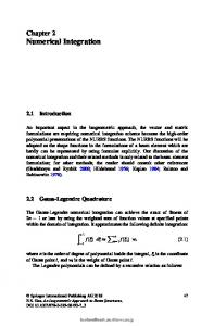
This algorithm can be extended to higher order quadratures by expanding the function sets G, F and H; or to integration over a higher dimensional curvilinear simplex by adding a further moment–fitting step. The complexity of the moment–fitting integration is optimal, e.g. O(1) of function evaluations per triangle. However, the weights computed by the fitting procedure are not necessarily all non-negative. There is no formal prove of the resulting quadrature accuracy as in (15) or the consistency order. Furthermore, in experiments we observe that the finite element methods with stiffness matrices assembled using moment–fitting can be less stable compared to applying other numerical integration techniques discussed here. Below we consider another integration method of optimal complexity. e and denote by p1 , p2 the intersection points of ∂Ωh Consider the curvilinear remainder Q with QK . If there are more than 2 such points, then the calculations below should be repeated e Choose points {qi } on (p1 , p2 ) as a nodes for each of the simply-connected component of Q. of a Gaussian quadrature with weights {ωi }. Consider the normal vector n for the line passing ˆ i on the boundary such that through p1 and p2 . For each point qi , one finds the point q ˆ i = qi + αn, α ∈ R, and φh (ˆ q qi ) − c0 = 0, where c0 is the φh -level value for ∂Ωh , i.e. c0 = 0 for ˆ i up to machine precision the FEM (9) and c0 = ±dh for the FEM (10). Secant method finds q within a few steps. Further we employ the same 1D quadrature rule to place points {rij } on e is computed through ˆ i ). The integral over Q each segment (qi , q Z X X ˆ i |sign(φh (qi ))ωi sign(φh )f (x)dx ≈ Ih,Qe (f ) = |p1 − p2 | |qi − q f (rij )ωj . (19) e Q

i

j

ˆ i |sign(φh (qi ))ωi ωj The weights for integrating over Q mayPbeP combined in ωij = |p1 − p2 ||qi − q to write the final quadrature formula i j f (rij )ωij . We remark that for problem (10), the 9

factor sign(φh (qi )) in (19) is replaced by sign(φh (qi ) + dh ) or sign(dh − φh (qi )) depending on the level set of ∂Ωh . Similar to the moment–fitting method, the complexity of the numerical integration is optimal, i.e. O(1) of function evaluations per triangle. All weights ωij are positive, and the accuracy analysis of numerical integration of a smooth function over Ω, which invokes the constructed quadrature for handling boundary terms, is straightforward and outlined below. We estimate the error of integration of a sufficiently smooth f over Ω. The integration uses a conventional quadrature scheme for interior cells of Th and the quadrature (19) for the curvilinear remainders of cut cells. This composed numerical integral is denoted by Ih,K (f ). Assume the 2D quadrature over regular triangles has O(hm ) accuracy. By the triangle inequality, we have Z Z Z Z f dx − Ih,Ω (f ) ≤ f dx − f dx − Ih,Ω (f ) f dx + Ω

Ω

Ωh

Ωh

We apply the co-area formula to estimate the first term Z Z f dx − Ω

Ωh

f dx ≤

Z

Z |f |dx ≤ kf kL∞

(Ω4Ωh )

1dx (Ω4Ωh ) +kφhZ−φkL∞

Z

≤ kf kL∞

|∇φ|dxdt ≤ Chq kf kL∞ .

−kφh −φkL∞ {φ=t}

For the second term we estimate Z X Z , ≤ f dx − I (f ) f dx − I (f ) h,K h,Ω Ωh

K∈Th

K

where Ih,K (f ) is a quadrature we use to integrate f over K ∩ Ωh . Decomposing the mesh into interior cells Thint and cut cells ThΓ (those intersected by ∂Ωh ) and applying triangle inequalities, we obtain: Z X Z X Z f dx − Ih,K (φh , f ) . f dx − Ih,Ω (f ) ≤ f dx − Ih,K (f ) + Ωh

K∈Thint

K

K∈ThΓ

K∩Ωh

The interior cells are integrated with the error Chm by a conventional method: X Z f dx − Ih,K (f ) ≤ Chm . K∈Thint

K

eK , Q e K = Q4QK and polygonal QK defined earlier, we have For Q = K ∩ Ωh = QK ∪ Q X Z X Z ≤ Chm + f dx − I (φ , f ) | sign(φh )f dx − IQeK (f )|. h,K h e K∈ThΓ

K∩Ωh

K∈ThΓ

QK

The estimate below assumes that a Gaussian 1D quadrature with P nodes is used in the construction of (19). For each interval (p1 , p2 ) we introduce the local orthogonal coordinate system (s, t) = x(s) + tn, where s : (0, |p2 − p1 |) → (p1 , p2 ) parameterizes the interval. The

10

graph of the zero level of φh is the implicit function γ(s) given by φh (x(s) + γ(s)n) = 0. We note the identity d2P ds2P

Z

2P −1 X

γ(s)

f (s, t) dt = 0

Ck2P

k=0

∂ k f d2P −k γ + ∂sk ds2P −k

Z 0

γ(s)

∂ 2P f (s, t) dt. ∂s2P

We assume f and γ(s) to be smooth enough that |

d2P ds2P

Z

γ(s)

f (s, t) dt| ≤ Cf ,

(20)

0

with a constant Cf uniform over all K ∈ ThΓ and independent of h. Applying standard estimates for the Gaussian quadratures, we get: Z Z p2 Z γ(s) XX XX f (s, t)dtds − ωij f (rij )| | sign(φh )f dx − ωij f (rij )| = | eK Q

i

≤|

i

≤

p1

j

XZ

X

γ(qi )

f dt −

0

X

0

i

j

ωij f (rij )| + C |p1 − p2 |h(2P )

(21)

j

C |γ(qi )|kf kW 2P,∞ h(2P ) + C h(2P +1) ≤ C h(2P +1) .

i

For a 2D boundary, the number of unfitted regions Q grows at an order of O(h−1 ). Then the entire error for all unfitted regions will be O(h2P ). To satisfy (15), it is sufficient to set 2P + 1 = m ≤ q + 2. Therefore, for sufficiently smooth f the assumption (20) is valid if γ(s) ∈ W q+1,∞ with the W q+1,∞ -norm uniformly bounded over all cut triangles and independent of h. The latter follows from our assumptions on φh and φ. Indeed, let Jh (φ) be a suitable polynomial interpolant for φ on a cut triangle K. By triangle inequality we have kφh kW q+1,∞ (K) ≤ kφh − Jh (φ)kW q+1,∞ (K) + kφ − Jh (φ)kW q+1,∞ (K) + kφkW q+1,∞ (K) .

(22)

Applying the finite element inverse inequality, condition (5), estimate (6) and approximation properties of polynomials we get for the first term on the right-hand side of (22): kφh − Jh (φ)kW q+1,∞ (K) ≤ C h−q kφh − Jh (φ)kW 1,∞ (K) ≤ C h−q (kφh − φkW 1,∞ (K) + kφ − Jh (φ)kW 1,∞ (K) ) ≤ C , with a constant C independent of K and h. Estimating the second and the third terms on the right-hand side of (22) in an obvious way, we obtain kφh kW q+1,∞ (K) ≤ C ,

(23)

with a constant C independent of K and h. The desired estimate on the W q+1,∞ -norm of γ follows from (23), the properties of implicit function and assumptions on φ.

4

Numerical examples

In this section we demonstrate the results of a few experiments using different numerical integration approaches described in the previous section. 11

4.1

Integral of a smooth function

We first experiment with computing integral of a smooth function over an implicitly defined domain in R2 . For the domain we choose the annular region defined by the level set function φ(x) = | |x| − 1| − 0.1,

Ω = {x ∈ R2 : φ(x) < 0}.

For f given in polar coordinates by f (r, θ) = 105 sin(21θ) sin(5πr). R the exact value Ω f dx is known and can be used to test the accuracy of different approaches. Due to the symmetry, the computational domain is taken to be the square Ωbulk = (0, 1)2 . Further, uniform triangulation with meshes of sizes h = 0.1 × 2−i , i = 0, . . . , 8, are built to triangulate Ωbulk . To avoid extra geometric error and assess the accuracy of numerical integration, in these experiments we set φh = φ. All four methods are set up to deliver the local error estimate (15) with m = 4 or m = 5. This should lead to O(h3 ) and O(h4 ) global accuracy, respectively. Tables 1–4 demonstrate that all methods demonstrate convergent results with local parametrization and sub-triangulation being somewhat more accurate in terms of absolute error values. At the same time, only moment–fitting and local parametrization approaches are optimal in terms of the computational complexity. Here we measure complexity in terms of the number of function evaluations. The total number of function evaluations to compute integrals over cut elements and interior elements is shown. Monte-Carlo method appears to be the most computationally expensive. Both Monte-Carlo and sub-triangulation methods become prohibitively expensive for fine meshes so that we make only 4 refining steps with those methods for m = 4 and only 2 refining steps for m = 5. The actual CPU timings (not shown) depend on particular implementation. For a Matlab code we used, the moment–fitting was the fastest among the four tested for a given h. h 0.1000 0.0500 0.0250 0.0125 0.0062 0.0031 0.0016 0.0008 0.0004

MF 7.41e+01 6.22e+00 9.14e-02 7.96e-03 1.28e-03 9.05e-06 1.11e-05 4.17e-08 1.68e-07

rate 3.57 6.09 3.52 2.64 7.14 -0.29 8.06 -2.01

MC 5.50e-01 4.78e-02 1.56e-03 7.93e-04 1.22e-04

rate 3.52 4.94 0.98 2.70

ST 1.02e-01 8.53e-03 4.80e-04 1.35e-05 1.17e-06

rate 3.58 4.15 5.15 3.53

LP 1.66e+00 7.06e-03 4.46e-03 5.91e-05 1.18e-05 2.62e-07 3.99e-08 1.91e-09 1.44e-10

rate 7.88 0.66 6.24 2.32 5.49 2.72 4.38 3.73

Table 1: The global error and the error reduction rates for the numerical integration using moment–fitting (MF), Monte-Carlo (MC), sub-triangulation (ST), and local parametrization (LP) algorithms to handle cut elements. The table shows results with m = 4.

4.2

Unfitted FEM

In the next series of experiments we solve the Poisson equation with Neumann’s boundary condition in the unit disc domain defined implicitly as Ω = {x ∈ R2 : φ(x) < 0} with φ = |x|−1. We are interested in solving (2) with α = 1 and the right-hand side given in polar coordinates by f = (a2 + r−2 + 1) sin(aθ) sin(θ) − a/r cos(ar)sin(θ) + (c2 + 1) cos(cr) + c/r sin(cr). 12

h 0.1000 0.0500 0.0250 0.0125 0.0062 0.0031 0.0016 0.0008 0.0004

MF 1 352 3 718 11 726 40 144 146 926 561 912 2 194 452 8 671 104 34 471 164

MC 25 802 93 491 346 005 1 342 357 40 645 578 -

ST 4 136 16 966 68 942 277 456 1 113 070

LP 423 1 608 12 750 42 192 151 022 570 104 2 210 836 8 703 872 34 536 700

Table 2: The number of function evaluations for the numerical integration using moment–fitting (MF), Monte-Carlo (MC), sub-triangulation (ST), and local parametrization (LP) algorithms to handle cut elements. The table shows results with m = 4. h 0.1000 0.0500 0.0250 0.0125 0.0062 0.0031

MF 2.80e+01 2.79e-01 4.44e-03 3.61e-04 2.11e-05 9.59e-07

rate 6.65 5.97 3.62 4.10 4.46

MC 6.49e-02 8.64e-04

rate 6.23

ST 5.51e-02 7.60e-03 2.25e-05

rate 2.86 8.40

LP 4.16e-02 1.13e-04 7.18e-06 9.75e-09 1.53e-09 7.73e-12

rate 8.52 3.98 9.52 2.67 7.63

Table 3: The global error and the error reduction rates for numerical integration using moment– fitting (MF), Monte-Carlo (MC), sub-triangulation (ST), and local parametrization (LP) algorithms to handle cut elements. The table shows results with m = 5. The corresponding solution is u(r, θ) = sin(ar) sin(θ) + cos(cr). In experiments we set a = 7π/2 and c = 3π . The bulk domain Ωbulk = (− 32 , 32 )2 is triangulated using uniform meshes of sizes h = 0.5×2−i , i = 0, . . . , 8. We experiment with P2 and P3 finite elements. The discrete level set function is the finite element interpolant to the distance function φ, φh = Jh (φ). Hence, the estimate (6) holds with q = 2 and q = 3, respectively. To be consistent with the geometric error and polynomial order, all four integration methods for cut cells were set up to deliver the local error estimate (15) with m = 4 and m = 5, respectively. According to (11), we should expect O(h2 ) and O(h3 ) convergence in the energy norm and O(h3 ) and O(h4 ) convergence in the L2 (Ω) norm. Figure 3 shows the error plots for the unfitted finite element method (9) for different mesh sizes. The results are shown with the moment–fitting and local parametrization algorithms used for the integration over cut triangles. The FE errors for Monte-Carlo and sub-triangulation were very similar to those obtained with the local parametrization quadratures and hence they are not shown. These results are in perfect agreement with the error estimate (11). Interesting that using the moment–fitting method for computing the stiffness matrix and the right-hand side leads to larger errors for the computed FE solution. Further, Figure 4 shows the CPU times needed for the setup phase of the finite element method using different numerical integration tools. For P2 element, the moment–fitting, the local parametrization and the sub-triangulation method show similar scaling with respect to h since the complexity is dominated by the matrix assemble over internal triangles, while for P3 elements local parametrization is superior in terms of final CPU times. As expected from the above analysis, the Monte–Carlo algorithm is non-optimal in either case.

13

h 0.1000 0.0500 0.0250 0.0125 0.0062 0.0031

MF 1 352 3 718 11 726 40 144 146 926 561 912

MC 2 341 229 117 184 420

ST 38 696 308 806 2 465 102

LP 1 928 4 870 14 030 44 752 156 142 580 344

Table 4: The number of function evaluations for numerical integration using moment–fitting (MF), Monte-Carlo (MC), sub-triangulation (ST), and local parametrization (LP) algorithms to handle cut elements. The table shows results with m = 5.

Figure 3: Finite element method error for P2 (left) and P3 (right) elements. The error plots are shown for moment–fitting (MF) and local parametrization (LP) used to treat cut elements.

4.3

Narrow-band unfitted FEM

In the final series of experiments we apply the narrow-band unfitted finite element method (10) to solve the Laplace-Beltrami equation (3) with α = 1 on the implicitly defined surface Γ = {x ∈ R2 : φ(x) = 0} with φ = |x| − 1. The solution and the right-hand side are given in polar coordinates by u = cos(8θ), f = 65 cos(8θ). The bulk domain, triangulations and the discrete level set function are the same as used in the previous series of experiments in section 4.2. For the extended finite element formulation (10) we define the following narrow band domain: Ωh = {x ∈ R2 : |φh (x)| < 2h}. The extension of the right-hand side is done along normal directions to Γ. For the discrete Hessian in Ωh , we take the exact one computed by Hh := ∇2 φ in Ωh . Finite element space Vh is the same as in section 4.2 and is build on P2 or P3 piecewise polynomial continuous functions in Ωbulk . Similar to the previous test case, four integration methods for cut cells were set up to deliver the local error estimate (15) with m = 4 and m = 5, respectively. According to (13), we should expect O(h2 ) and O(h3 ) convergence in the energy norm. Although there is no error estimate proved in the L2 norm, the optimal convergence order would be O(h3 ) and O(h4 ).

14

Figure 4: Dependence of the total CPU time to assemble stiffness matrices for P2 (left) and P3 (right) elements. Times are shown for moment–fitting (MF), local parametrization (LP), sub-triangulation (ST) and Monte-Carlo (MC) methods used to treat cut elements.

Figure 5: L2 (Γ) and H 1 (Γ) errors for the narrow-band with P2 (left) and P3 (right) bulk elements. The error plots are shown for moment–fitting (MF) and local parametrization (LP) used to treat cut elements. Figure 5 shows the error plots for the narrow-band unfitted finite element method (9) for different mesh sizes. All errors were computed over Γ as stands in the estimate (13), rather than in the bulk. The results are shown only for the moment–fitting and local parametrization algorithms used for the integration over cut triangles. As before, the results with other methods were very similar to those obtained with the local parametrization quadratures. The results with local parametrization are in perfect agreement with the error estimate (13) and predict the gain of one order in the L2 (Γ) norm. Using the moment–fitting leads to unstable results in the case of quadratic finite elements and to sub-optimal convergence in the case of cubic elements. Note that in these two cases moment–fitting with quadratic and cubic basis G, respectively, were used.

15

5

Conclusions

Building higher order quadrature rules for the numerical integration over implicitly defined curvilinear domains remains a challenging problem, important in many applications of unfitted finite element methods. Well known approaches are not robust with respect to how a surface cuts the mesh or have non-optimal computational complexity. In this paper we studied two methods of optimal complexity, namely, the moment–fitting and the local parametrization. Although moment–fitting delivers optimal accuracy for the integration of a smooth function over a bulk curvilinear domain, its application to numerical PDEs were found to produce sub-optimal results. Local parametrization provides accurate and stable integration method. However, its extension to 3D problems is not straightforward and requires further studies. Developing more stable versions of the moment–fitting method, extending parametrization technique to higher dimensions, or devising ever different numerical approaches to (1) all can be directions of further research.

References [1] A. Abedian, J. Parvizian, A. Duester, H. Khademyzadeh, and E. Rank, Performance of different integration schemes in facing discontinuities in the finite cell method, International Journal of Computational Methods, 10 (2013), p. 1350002. [2] A. Agouzal and Y. Vassilevski, On a discrete hessian recovery for p1 finite elements, Journal of Numerical Mathematics, 10 (2002), pp. 1–12. [3] J. W. Barrett and C. M. Elliott, A practical finite element approximation of a semi-definite Neumann problem on a curved domain, Numerische Mathematik, 51 (1987), pp. 23–36. [4] T. Belytschko and T. Black, Elastic crack growth in finite elements with minimal remeshing, International journal for numerical methods in engineering, 45 (1999), pp. 601– 620. [5] E. Burman, S. Claus, P. Hansbo, M. G. Larson, and A. Massing, Cutfem: discretizing geometry and partial differential equations, International Journal for Numerical Methods in Engineering, 104 (2015), pp. 472–501. [6] E. Burman and P. Hansbo, Fictitious domain finite element methods using cut elements: Ii. a stabilized Nitsche method, Applied Numerical Mathematics, 62 (2012), pp. 328–341. [7] E. Burman, P. Hansbo, and M. G. Larson, A stabilized cut finite element method for partial differential equations on surfaces: The Laplace–Beltrami operator, Computer Methods in Applied Mechanics and Engineering, 285 (2015), pp. 188–207. ´au, N. Chevaugeon, and N. Moe ¨s, Studied X-FEM enrichment to handle ma[8] K. Dre terial interfaces with higher order finite element, Computer Methods in Applied Mechanics and Engineering, 199 (2010), pp. 1922–1936. [9] T.-P. Fries and T. Belytschko, The extended/generalized finite element method: an overview of the method and its applications, International Journal for Numerical Methods in Engineering, 84 (2010), pp. 253–304. ´, Higher-order accurate integration of implicit geometries, [10] T.-P. Fries and S. Omerovic International Journal for Numerical Methods in Engineering, (2015). 16

[11] J. Grande and A. Reusken, A higher-order finite element method for partial differential equations on surfaces, Preprint, 401 (2014). [12] S. Gross, M. A. Olshanskii, and A. Reusken, A trace finite element method for a class of coupled bulk-interface transport problems, ESAIM: Mathematical Modelling and Numerical Analysis, 49 (2015), pp. 1303–1330. [13] D. J. Holdych, D. R. Noble, and R. B. Secor, Quadrature rules for triangular and tetrahedral elements with generalized functions, International Journal for Numerical Methods in Engineering, 73 (2008), pp. 1310–1327. [14] T. J. Hughes, J. A. Cottrell, and Y. Bazilevs, Isogeometric analysis: CAD, finite elements, NURBS, exact geometry and mesh refinement, Computer methods in applied mechanics and engineering, 194 (2005), pp. 4135–4195. [15] C. Min and F. Gibou, Geometric integration over irregular domains with application to level-set methods, Journal of Computational Physics, 226 (2007), pp. 1432–1443. [16] R. Mittal and G. Iaccarino, Immersed boundary methods, Annu. Rev. Fluid Mech., 37 (2005), pp. 239–261. ´ Be ´chet, S. P. Bordas, D. Quoirin, and [17] M. Moumnassi, S. Belouettar, E. M. Potier-Ferry, Finite element analysis on implicitly defined domains: An accurate representation based on arbitrary parametric surfaces, Computer Methods in Applied Mechanics and Engineering, 200 (2011), pp. 774–796. ¨ ller, F. Kummer, and M. Oberlack, Highly accurate surface and volume inte[18] B. Mu gration on implicit domains by means of moment-fitting, International Journal for Numerical Methods in Engineering, 96 (2013), pp. 512–528. [19] M. A. Olshanskii, A. Reusken, and J. Grande, A finite element method for elliptic equations on surfaces, SIAM Journal on Numerical Analysis, 47 (2009), pp. 3339–3358. [20] M. A. Olshanskii and D. Safin, A narrow-band unfitted finite element method for elliptic pdes posed on surfaces, Math. Comp., doi: 10.1090/mcom/3030. [21] R. Saye, High-order quadrature methods for implicitly defined surfaces and volumes in hyperrectangles, SIAM Journal on Scientific Computing, 37 (2015), pp. A993–A1019. [22] A.-K. Tornberg, Multi-dimensional quadrature of singular and discontinuous functions, BIT Numerical Mathematics, 42 (2002), pp. 644–669. [23] M.-G. Vallet, C.-M. Manole, J. Dompierre, S. Dufour, and F. Guibault, Numerical comparison of some hessian recovery techniques, International Journal for Numerical Methods in Engineering, 72 (2007), pp. 987–1007.

17