Numerical Solution of Extended Block Backward ... - Semantic Scholar

Proceedings of the World Congress on Engineering 2012 Vol I WCE 2012, July 4 - 6, 2012, London, U.K.

Numerical Solution of Extended Block Backward Differentiation Formulae for Solving Stiff ODEs S. A. M. Yatim, Z. B. Ibrahim, K.I. Othman and M. B. Suleiman  Abstract—Existing Block Backward Differentiation Formulae (BBDF) of different orders are collected based on their competency and accuracy in solving stiff ordinary differential equations (ODEs). The strategy to fully utilize the formulae is optimized using variable step variable order approach. The improved performances in terms of accuracy and computation time are presented in the numerical results with different sets of test problems. The comparison is made between the proposed method and MATLAB’s suite of ordinary differential equations (ODEs) solvers namely ode15s and ode23s. Index Terms— Numerical Analysis, Initial Value Problem, Ordinary Differential Equations, Stiff ODEs, BBDF methods

I. INTRODUCTION

M

OTIVATED by applied problems arise from physical, biological and physical phenomenon, there are numbers of researches commenced to devise effective and very accurate methods to solve stiff ODEs [1]. Gear’s method which is associated with backward differentiation formula (BDF) in [2] has presented promising results in certain point of comparison. Some popular codes based on BDF include LSODE and VODE. The most recent code associated with BDF is called MEBDF presented in [3] has also discussed its performance on a large set of stiff tests problems. Because of a broad class of problems occurred in applied sciences [4]-[7], the methods are developed giving rigorous results in terms of accuracy and computation time. The study of numerical methods for solving stiff initial value problems for ODEs is said to have reached a certain maturity. Many in recent papers have tried to describe and compare some of the best codes available [8]. Because of that, there now exist some excellent codes which are both efficient and reliable for solving these particular classes of

Manuscript received March 6, 2012; revised April 5, 2012. Z.B. Ibrahim is with the Department of Mathematics, Faculty of Science, Universiti Putra Malaysia, 43400 UPM Serdang, Selangor, Malaysia. (phone: +603-89466861; e-mail: [email protected]). S. A. M. Yatim is with the Department of Mathematics, Faculty of Science, Universiti Putra Malaysia, 43400 UPM Serdang, Selangor, Malaysia. K. I. Othman is with the Department of Mathematics, Faculty of Computer and Mathematical Sciences, Universiti Teknologi MARA, 40450 Shah Alam, Selangor, Malaysia. M. B. Suleiman is with the Department of Mathematics, Faculty of Science, Universiti Putra Malaysia, 43400 UPM Serdang, Selangor, Malaysia.

ISBN: 978-988-19251-3-8 ISSN: 2078-0958 (Print); ISSN: 2078-0966 (Online)

problems. A crucial component in developing an efficient ODE solver is by taking into accounts their accuracy, rate of convergence, and computation time. This is of great importance in situation example in astronomy, when longterm, very accurate and reliable numerical solution is sought. The study on BBDF was first introduced in [9] demonstrates the competency of computing concurrent solution values at different points. Consequently, study in [10] is extended in a way that the accuracy is improved by increasing the order of the method up to order 5 [11]. Thus, BBDF of order 3 to 5 are collected and we introduce variable step variable order approach to its strategy in choosing the stepsize. We are interested to compare the numerical results obtained with stiff ODEs solvers available in Matlab; ODE15s and ODE23s. The problems considered in this paper are for the numerical solution of the initial value problem,

y   f ( x, y )

(1)

with given initial values y ( a )  y 0 in the given interval

x  [a, b] .

II. DERIVATION OF EXTENDED BLOCK BACKWARD DIFFERENTIATION FORMULAE METHOD

A. Construction of Extended Block Backward Differentiation Formulae method

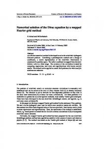
Fig 1. Extended BBDF method of order (P3-P5)

WCE 2012

Proceedings of the World Congress on Engineering 2012 Vol I WCE 2012, July 4 - 6, 2012, London, U.K.

Two values of yn1 and y n 2 were computed simultaneously in block by using earlier blocks with each block containing a maximum of two points (Fig 1). The orders of the method (P3, P4 and P5) are distinguished by the number of backvalues contained in total blocks. The ratio distance between current ( xn ) and previous step ( xn1 ) is represented as r and q in Fig 1. In this paper, the step size is given selection to decrease to half of the previous steps, or increase up to a factor of 1.9. For simplicity, q is assigned as 1, 2 and 10/19 for the case of constant, halving and increasing the step size respectively. The zero stability is achieved for each of these cases and explained in the next section. We find approximating polynomials Pk (x) , by means of a k-degree polynomial interpolating the values of y at given points are ( xn 3, yn3 ) , ( xn 2, yn2 ) , ( xn1, yn1) …, ( x n 2 , y n 2 ) .

Pk   j 0 y ( x n 1 j ).Lk , j ( x) k

(2)

where k

Lk , j ( x) 

(x  x

 ( x n1 j nx1ni 1i ) )

i 0 i j

for each j  0,1,..., k The interpolating polynomial of the function y (x) using Lagrange polynomial in (2) gives the following corrector for the first point y np1 , and second point y np 2 . The resulting Lagrange polynomial for each order was given as follows: For Extended BBDF of order P3 ( P  3 )

For Extended BBDF of order P5 ( P  5 ) P( x)  P ( xn 1  sh) (q  2r  1  s )(2r  1  s )(r  1  s )(1  s ) s yn  2 2(q  2r  2)(2r  2)(r  2) (q  2r  1  s )(2r  1  s )(r  1  s )(1  s )( s  1)  yn 1 (q  2r  1)(2r  1)(r  1) (q  2r  1  s )(2r  1  s)(r  1  s ) s ( s  1) (5)  yn 2 4(q  2r )r (q  2r  1  s )(2r  1  s )(1  s ) s ( s  1)  yn 1  r 2 (q  r )( r  1)( r  2) (q  2r  1  s )(r  1  s )(1  s ) s ( s  1)  yn  2 2qr 2 (2r  1)(2r  2) (2r  1  s )(r  1  s )(1  s ) s ( s  1)  yn  3  q (q  r )(q  2r )(q  2r  1)( q  2r  2)



By substituting s  0 and s  1 gives the corrector for the first and second point respectively. Therefore by letting r  1, q  1 , r  2, q  2 and r  1, q  10 / 19 we produced the following equations for the first and second point of Extended BBDF. Extended BBDF of order P3 ( P  3 ) When r  1, q  1

y n 1  2hf n 1  y n 2 

When r  2, q  2

y n 1  3hf n 1 

P( x)  P( xn 1  sh) (r  1  s)( s  1)( s) (r  1  s)( s  1)( s  1)  yn  2  yn 1 (3) 2r  4 1  r (r  1  s)( s  1)( s) (1  s)( s  1)( s)  yn  yn 1 2r r (1  r )(r  2)

y n2 

4 hf n  2 7

9 9 1 y n  2  y n  y n 1 8 4 8 32 4 1  y n 1  y n  y n 1 21 7 21

When r  1, q  10 / 19

29 841 841 361 hf n 1  y n2  yn  y n 1 19 1824 380 480 48 4608 576 6859  hf n  2  y n 1  yn  y n 1 91 2639 455 13195

y n 1 

y n 2

For Extended BBDF of order P4 ( P  4 ) P ( x)  P( xn 1  sh)

(2r  1  s )(r  1  s )(1  s )( s ) yn  2 2(2r  2)(r  2) (2r  1  s )(r  1  s )(1  s )( s  1)  yn 1 (2r  1)(r  1) (2r  1  s )(r  1  s )( s )( s  1)  yn 4r 2 (2r  1  s )(1  s )( s )( s  1)  yn 1 r 2 ( r  1)(r  2) (r  1  s )(1  s )( s )( s  1)  yn  2 2r 2 (2r  1)(2r  2)

6 hf n  2 11

2 1 y n  2  2 y n  y n 1 3 3 18 9 2  y n 1  y n  y n 1 11 11 11

Extended BBDF of order P4 ( P  4 ) When r  1, q  1



6 3 9 3 1 hf n 1  y n  2  y n  y n 1  y n2 5 10 5 5 10 12 48 36 16 3  hf n2  y n1  y n  y n1  y n2 25 25 25 25 25

y n 1  yn2

When r  2, q  2 (4)

15 75 225 25 3 hfn1  y n 2  yn  yn1  y n 2 8 128 128 128 128 12 192 18 3 2  hfn2  yn1  yn  yn1  y n2 23 115 23 23 115

yn1 

yn2

When r  1, q  10 / 19

ISBN: 978-988-19251-3-8 ISSN: 2078-0958 (Print); ISSN: 2078-0966 (Online)

WCE 2012

Proceedings of the World Congress on Engineering 2012 Vol I WCE 2012, July 4 - 6, 2012, London, U.K.

Are said to be of order p if c o  c1  ...  c p  0 , C p 1  0 . The general form for the

1131 14703 1279161 hf n 1  yn  2  yn 1292 82688 516800 183027 10469  yn 1  yn  2 108800 27200 1392 89088 242208  hf n  2  yn 1  yn 3095 40235 77375 198911 658464  yn 1  yn  2 77375 1005875

yn 1 

yn  2

constant C q is defined as j

Cq 

q  2,3,... p  1 (7)

Consequently, BBDF method can be represented in standard form by an equation k

k

j 0

j 0

 A j yn  j  h  B j f n  j

where A j and B j are r by r

matrices with elements a l ,m and bl ,m for l , m  1,2,...r .

12 12 24 12 hf n 1  yn  2  yn  yn 1 13 65 13 13 4 3  yn  2  yn  3 13 65 60 300 300 200  hf n  2  yn 1  yn  yn 1 137 137 137 137 75 12  yn  2  yn  3 137 137

yn 1 

Since Extended BBDF for variable order ( P ) is a block method, we extend the definition 3.2 in the form of j

 [ Ak z ( x  kh)  hBk z ' ( x  kh)]

L[ z ( x ); h] 

(8)

k 0

And the general form for the constant C q is defined as j

Cq 

When r  2, q  2

 [k q Ak  (q  1)! k q1 Bk ] q  2,3,... p  1 1

(9)

k 0

105 3675 3675 1225 hf n 1  yn  2  yn  yn 1 71 9088 2272 4544 147 75  yn  2  yn  3 2272 9088 24 3072 48 12  hf n  2  yn 1  yn  yn 1 49 1715 49 49 16 3  yn  2  yn 3 245 343

yn 1 

yn  2

1

k 0

Extended BBDF of order P5 ( P  5 ) When r  1, q  1

yn  2

 [k q k  (q  1)! k q 1 k ] ,

Ak is

equal

to

the

coefficients

of

y k where

k  n  ( P  2),..., n  1, n  2 and P  3, 4,5 . Throughout this section, we illustrate the effect of Newton-type scheme which in general form of

yn(i1,1)n2

 yn(i)1,n2

When r  1, q  10 / 19

402 13467 13467 13467 hf n 1  yn  2  yn  yn 1 449 77228 7184 13021 4489 7428297  yn  2 yn  3 8980 44792240

yn 1 

516 177504 5547 59168 hfn2  yn1  yn  yn1 1189 79663 2378 34481 5547 7428297  yn2  yn3 5945 23102270

yn2 

(I  A) yn(i)1,n2  hBF ( yn(i)1,n2 )        F  (I  A)  hB ( yn(i)1,n2 ) y   (10)

The general form of Extended BBDF method is yn 1  1hf n 1  1 yn  2  1   yn  2  1hf n  2  1 yn 1   2 

with

(11)

and

are the back values. By setting ,  y n 1  , , 1 0 , I   y n 1, n  2    0 1    y n2 

  0 ,  f n 1  , and  B 1 n1,n2   1   Fn 1, n  2   f  0  2   n2   2  Equation (11) in matrix-vector form is equivalent to

As similar to analysis for order of Linear Multistep Method (LMM) given in [12], we use the following definition to determine the order of Extended BBDF method. Definition 3.1 The LMM [12] and the associated difference operator L defined by

L[ z ( x); h] 

j

 [ k z ( x  kh)  h k z ( x  kh)] '

k 0

ISBN: 978-988-19251-3-8 ISSN: 2078-0958 (Print); ISSN: 2078-0966 (Online)

(6)

( I  A) y n 1, n  2  hBFn 1.n  2   n 1,n  2 Equation (12) is simplified as

(12)

fˆn 1,n  2  ( I  A) y n 1,n  2  hBFn 1,n  2   n 1,n  2  0 (13)

Newton system fˆ

iteration

n 1,n  2

is

performed

to

the

 0 , by taking the analogous form of (10)

where J n 1, n  2   F (Yn(i )1, n  2 ) , is the Jacobian matrix of  Y 

F with respect to Y . Equation (10) is separated to three different matrices denoted as WCE 2012

Proceedings of the World Congress on Engineering 2012 Vol I WCE 2012, July 4 - 6, 2012, London, U.K.

E1(,i21)  y n(i11,)n 2  y n(i)1,n  2

(14)

III. NUMERICAL RESULTS

F (i ) Aˆ  ( I  A)  hB (y ) Y n 1,n  2

(15)

Bˆ  ( I  A) y n(i)1,n  2  hBF ( y n(i)1,n  2 )   n 1,n  2

We carry out numerical experiments to compare the performance of Extended BBDF method with stiff ODE solvers in MATLAB mentioned earlier. These test problems are performed under different conditions of error tolerances – (a) 10-2, (b) 10-4 and, (c) 10-6

(16)

Two-stage Newton iteration works to find the approximating solution to (1) with two simplified strategies based on evaluating the Jacobian ( J n 1,n  2 ) and LU

The test problems and solution are listed below Problem 1 y '  100( y  x)  1 y (0)  1 0  x  10 With solution: y ( x)  e100 x  x

factorization of Aˆ [12].

Problem 2 B. Order and stepsize selection The importance of choosing the step size is to achieve reduction in computation time and number of iterations. Meanwhile changing the order of the method is designed for finding the best approximation. Strategies proposed in [13] are applied in this study for choosing the step size and order. The strategy is to estimate the maximum step size for the following step. Methods of order P-1, P, P+1 are selected depending on the occurrence of every successful step. Consequently, the new step size hnew is obtained from which order produces the maximum step size. The user initially will have to provide an error tolerance limit, TOL on any given step and obtain the local truncation error (LTE) for each iteration. The LTE is obtained from LTE k  y n( P 21)  y n( P )2 , P  3,4,5

y1'  1002 y1  1000 y 2 y1 (0)  1 0  x  10 y2'  y1  y2 (1  y2 ) y2 (0)  0

With solution: y1  e2 x y2  e  x

The abbreviations used in the following tables and figures are listed below: TS : the total number of steps taken TOL : the initial value for the local error estimate MAXE : the maximum error AVEE : the average error MTD : the method used TIME : the total execution time (seconds)

where yn( P21) is the ( P  1) -th order method and y n( P)2 is the -th order method. By finding the LTEs, the maximum step size is defined as 1

 TOL  P  h P 1  hold    LTE P 1 

 TOL h  hold   , P  LTE P

1

TABLE I NUMERICAL RESULTS FOR PROBLEM (1).

TOL 10-2

 P 1  , 

1

 TOL  P  2  h P 1  hold    LTE P 1 

10-4

Where hold is the stepsize from previous block and hmax is obtained from the maximum stepsize given in above equations. The successful step is dependent on the condition LTE