Object Boundary Detection in Images using a Semantic Ontology

Object Boundary Detection in Images using a Semantic Ontology Anthony Hoogs and Roderic Collins GE Global Research One Research Circle Niskayuna, NY 12309

{hoogs,collins}@research.ge.com

Abstract We present a novel method for detecting the boundaries between objects in images that uses a large, hierarchical, semantic ontology – WordNet. The semantic object hierarchy in WordNet grounds this ill-posed segmentation problem, so that true boundaries are defined as edges between instances of different classes, and all other edges are clutter. To avoid fully classifying each pixel, which is very difficult in generic images, we evaluate the semantic similarity of the two regions bounding each edge in an initial oversegmentation. Semantic similarity is computed using WordNet enhanced with appearance information, and is largely orthogonal to visual similarity. Hence two regions with very similar visual attributes, but from different categories, can have a large semantic distance and therefore evidence of a strong boundary between them, and vice versa. The ontology is trained with images from the UC Berkeley image segmentation benchmark, extended with manual labeling of the semantic content of each image segment. Results on boundary detection against the benchmark images show that semantic similarity computed through WordNet can significantly improve boundary detection compared to generic segmentation.

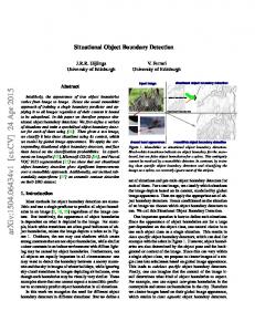
Figure 1: Top left: an image with a variety of objects. Top right: manual segmentation used for scoring. Bottom left: semantic distance segmentation, with score 0.70. Bottom right: visual distance segmentation, with score 0.63. Semantic segmentation emphasizes object-level differences even when visual distance is small, such as between the train and the bridge, and de-emphasizes edges within the same object such as the trees.

Introduction The goal of image boundary detection is to delineate boundaries between distinct objects in the scene while ignoring features interior to individual objects. One of the main challenges is that the boundary between two objects is a semantic distinction, supported by visual evidence that may be very weak. Hence higher-level, semantic information is often required to solve the segmentation problem effectively, but this information is not used by standard low-level segmentation processes such as edge detection and region segmentation (Malik et al. 2001). One solution is to assume the existence of a complete set of classes within the image domain, such that each pixel in the image can be uniquely labeled as belonging to one of the classes (Feng, Williams, & Felderhof 2002; Konishi & Yuille 2000). Then, given a correctly labeled image, class boundaries are the true boundaries, and other features such as additional edges are not.

This approach has a significant drawback, however. The pixel labeling problem, which is a form of generic object recognition, is even more difficult than the segmentation problem. In fact, the underlying premise of many segmentation algorithms is that detailed, class-level information is not required to perform segmentation (Malik et al. 2001). In this paper we explore a new method for image segmentation that uses sparse, class-level information, but without performing class recognition. Our underlying hypothesis is that boundaries can be detected using high-level semantic analysis, without attempting explicit pixel labeling or requiring class models. Partial, even erroneous object class hypotheses can provide useful evidence for making boundaryclutter decisions – evidence that is not available from image data alone. The basis of our method is the estimation of semantic distance between the two regions bounding an image edge. After an initial region segmentation based on intensity or color, each edge is bounded by exactly two regions. We hypothe-

c 2006, American Association for Artificial IntelliCopyright  gence (www.aaai.org). All rights reserved.

956

size that the semantic distance between the regions has a direct relationship to the probability that their common edge is a true boundary. This property allows two regions with very similar visual attributes, but from different object categories, to have a large semantic distance and therefore evidence of a strong boundary between them. Conversely, two regions with very different visual attributes, but from similar classes, should have a small semantic distance and therefore no boundary (see Figure 1). By mapping semantic distance into boundary probability, we produce an image segmentation that respects semantic distinctions, not just visual differences. Semantic distance is computed using WordNet, a large, hierarchical, semantic ontology commonly used in natural language (Fellbaum 1998) that provides object type-subtype relations for all noun senses in common English. WordNet is commonly used to compute semantic distance (Budanitsky & HirstWu 2001), but this is the first use of WordNet for image segmentation as far as we know. Typically, semantic information in visual classification problems is limited, quite literally, to a flat list of class labels (Chen & Wang 2002; Feng, Williams, & Felderhof 2002; Fei-Fei, Fergus, & Perona 2004). The major advantage of using a hierarchical taxonomy is that relatively sparse visual training data can be semantically generalized through the ontology. In effect, the ontology enables us to vastly undersample the range of object categories and visual appearance, which are enormous in general images, while still providing some notion of semantic distance. By the same token, our formulation of semantic distance is constrained to the relationships supported by the underlying ontology (type-subtype, or hyponymy, for WordNet). Other relationships, such as part-whole (meronymy) or coincidence of appearance, could also be used to either replace or complement our WordNet distance measure. Our results indicate that our semantic distance formulation does capture boundary saliency, and is effective for image segmentation. To train and test our method, we use the UC Berkeley Segmentation Benchmark (Martin & Malik ), which contains 300 images that have been manually segmented by 5+ people each. We have extended the benchmark data by selecting one segmentation per image, and manually labeling each region with its semantic content. The region labels correspond to WordNet noun sense definitions, so that visual features are linked to WordNet nodes. This dataset will be made publicly available, as it should be useful for categorical learning and evaluation. In this paper we do not propose a complete image segmentation solution. Edges with little gradient support may be missing from our segmentation, but there are methods to detect such boundaries (Yu 2005) There are also techniques for spatial and/or graphical regularization (Kumar & Hebert 2005) to add global constraints. The complete pixel labeling problem has been studied in constrained domains (Feng, Williams, & Felderhof 2002; Konishi & Yuille 2000) and in generic images with only image-level annotations for learning (Barnard et al. 2003). WordNet has been used for multimedia object recognition and video annotation (Hoogs et al. 2003), but not for image segmentation. Here, we address

the same open-ended, large-scale domain as (Barnard et al. 2003), but focus on the simpler problem of finding boundaries between objects. The next section outlines our approach to image segmentation using semantic distance. The visual appearance representation is then described, follow by comparative results on the Berkeley benchmark, and conclusions.

Computing Semantic Distance The semantic or conceptual distance between two objects is not equivalent to any particular measure of how different the objects appear in an image. When humans are asked to draw boundaries in an image to separate objects, our recognition capabilities enable grouping decisions that may directly contradict the visual evidence: combining wildly different fabric patterns into a single article of clothing, while perceiving and distinguishing camouflaging patterns in a lion’s pelt from the grasses in the background. Our basic procedure is relatively straightforward. First, we decompose the image into a region partition using a fast, non-semantic segmentation algorithm based solely on image intensity or color data. The partition forms a region graph such that each edge E is bounded by exactly two regions, R1 and R2 . Next, a feature vector Fi is computed for each region based on texture and color as described in the section on Visual Similarity. Then the semantic distance between R1 and R2 is estimated using the feature vectors and the learned appearance of semantic concepts in WordNet. Computing semantic distance does not require classification, as described below. To form the output segmentation, edges with small distances are given low probability (discarded), while those with large distances are retained. A semantic ontology enables the precise definition of the semantic distance between two concepts, independently of observed attributes. Note that in this work we use the term “semantic distance” to conform with the standard literature (Budanitsky & HirstWu 2001); we do not claim to have a metric distance, for example. For our semantic taxonomy, we use WordNet (Fellbaum 1998) because its hierarchical structure encodes semantic generalization/specialization of object types (noun sense hypernymy; we ignore meronyms, verbs, adjectives, etc.). The partitioning in WordNet is functional, rather than visual, physical, or geometric; this information cannot be learned from imagery alone, and complements the similarity cues derived from the visual data. The main challenge we address is how to estimate the semantic distance between two image features (regions) given WordNet and the low-level visual information available to segmentation algorithms. First, we augment WordNet with visual information from training images in an offline training stage. During segmentation, we index into the augmented WordNet using the visual information from the two regions. Finally, we compute the semantic distance between the indexed WordNet nodes. These steps are described in the following sections.

Augmenting WordNet with Visual Appearance As WordNet does not contain visual information, we use a set of labeling training images to add visual attributes to

957

Figure 3: Plots of the pdfs of semantic distance. The green curve is for all nodes that have exemplars in training. The red curve is for those nodes plus parent nodes with no exemplars.

Figure 2: A fragment of WordNet, with each node size approximately proportional to its probability in training.

children with exemplars. See Figure 2. WordNet nodes. Each training image is manually segmented into regions, and each region is manually labeled with the most specific WordNet concept describing its content. Each image is then segmented (again) using a low-level region segmentation algorithm (in this work, mean-shift (Comaniciu & Meer 2002)). We use the 200 training images from the Berkeley segmentation benchmark, which are provided with manual segmentations, and have added the semantic labels for each region. A feature vector is computed for each computed region and associated with the WordNet node matching the label. (In the case where a machine-segmented region overlaps multiple ground-truth labels, the label associated with the most pixels is used.) After all training images are processed, each node C may contain any number NC of exemplar feature vectors, including zero. To compute semantic distance, we require the prior probability αC for each node. We define this recursively as the sum of a node’s probability plus that of its children,  NC αC = + αS (1) NT

Estimating Semantic Distance Semantic distance can now be computed between any two nodes in the segmentation tree. More abstractly, all we require for semantic distance is a tree with weights on the graph edges. Each edge weight w is the ratio of childparent probability, w = αC /αP where C is a direct child of P . Note that 0 ≤ w ≤ 1, as we define w = 0 when αC = αP = 0. We compute the pairwise semantic distance Di,j between nodes Ci and Cj by finding their nearest common ancestor C0 . Let Ai,0 be the list of edges along the path from Ci to C0 ; likewise for Aj,0 . Then the semantic distance is   (1 − we ) + (1 − we ), (2) Di,j = e∈Ai,0

e∈Aj,0

which is the sum of one minus the child/parent probability ratios from each child Ci and Cj to the common ancestor C0 . This formulation has the desirable property that the distance increases with semantic difference as represented by the concept priors. For example, the semantic distance between a child C and parent P is 1 − (αC /αP ). When one child contains all of exemplars among the children of P , and P has no exemplars of its own, then DC,P = 0. This occurs for “otter” and “musteline mammal” in Figure 2; all of training examples are on “otter” and hence the two nodes are the same size. If C contains a small fraction of the exemplars of P and its children, then DC,P approaches one. Figure 3 shows the distribution of semantic distances between all nodes in the segmentation tree. This method differs from those evaluated in (Budanitsky & HirstWu 2001), because we sum weights along the path between the nodes, and we accumulate concept priors from both children and training. Now, we estimate the semantic distance between two regions R1 , R2 separated by an (image) edge E as follows: Compute the two feature vectors, F1 , F2 for the regions.

S∈SC

where SC is the set of children of C and NT is the total number of regions in training. Note that NC accounts for the situation where a node has exemplars as well as children with exemplars. One issue to be addressed is that WordNet is not a tree structure; when the path up from a child leads through multiple parents, we use the probability count that maximizes diversity in the ancestor node by eliminating paths which have higher proportions of weights from the child node. The result of this WordNet augmentation is a tree where each node has a prior probability and a list of visual feature vectors. We call the resulting tree the segmentation tree. At its root the probability is unity, reflecting that all concepts seen in training exist in the tree. Our augmented tree contains 6835 regions with 217 unique labels; the resulting WordNet tree contains 497 nodes that have exemplars or

958

Compute a distance measure D between F1 and every training exemplar in the segmentation tree; in our experiments, we use the χ2 -distance because our feature vectors are histograms as described below. Select the nodes S1 corresponding to the top K matches (in this work, K = 40). Each member in S1 represents a vote for the semantic class in the associated node in the tree. Repeat the process for F2 , generating S2 . The two sets are compared by computing the semantic distance between each member of one set against each member of the other. Each distance is mapped into a boundary probability using a non-linear function that controls the relationship of D and boundary strength, and the average is taken over the votes:  2 Di,j − µ 1 ) (3) tan−1 ( P (E) = − 2 πK(K − 1) σ

Figure 4: Plot of visual distance (red plus-signs) and groundtruth semantic distance (green crosses) for all computed edges in testing. The edges are sorted by semantic distance D; about 60% have D = 0. Note that 1) on average, visual distance is greater for edges with non-zero semantic distance; 2) non-zero semantic distance and visual distance are uncorrelated.

i∈S1 ,j∈S2

where the sum excludes duplicate pairings (hence the normalization is not K 2 ), and µ, σ are control parameters. Each pixel in E in the output boundary image is assigned the value P (E). After all edges are processed, the boundary image is complete. The purpose of using the K nearest neighbors is to handle noise in the matching process. As the visual features available to each region are low-level, local and ambiguous, each region may match a number of nodes distributed throughout the tree. If the two regions are truly from different classes, then the overall distribution of their matches should be different, even when they are visually similar, leading to a high average semantic distance. If the regions are from the same or semantically similar classes, then their match distributions should be similar. The mapping through tan−1 accounts for the intuitive notion that differences in semantic distance are more important when D is small. Once D increases sufficiently, the edge is highly likely to be a boundary regardless of further increases in D.

method, which we will call visual distance, directly compares the texton histograms H1 and H2 corresponding to R1 and R2 , using the χ2 histogram difference measure linearly mapped into edge strength, i.e. the pixels on edge E are assigned this value in the boundary image. We use this method as a baseline for comparison to semantic boundary detection. This method does quite well, achieving an overall F-score of 0.62 on the UCB benchmark. The highest published score we are aware of is 0.65 (Martin, Fowlkes, & Malik 2003), and most methods score below 0.59.

Experiments and Results In our experiments we examine the behavior of the semantic distance segmentation method (SDS) on the UC Berkeley segmentation benchmark. The benchmark is particularly useful here, because it defines a rigorous method for evaluating and comparing boundary detection algorithms. We follow the official benchmark paradigm by using the 200 designated training images, and 100 designated test images. We use the scoring software provided with the benchmark; it quantifies the match between a computed segmentation and multiple human segmentations by producing a precisionrecall curve and its corresponding F-score (harmonic mean of precision and recall). All reported results are on the 100 color test images unless specified otherwise. As mentioned above, we have augmented the benchmark by adding a semantic WordNet label to each region in one manual segmentation for each of the 300 images. First, we establish an upper bound on the performance possible with SDS. Then we show the improvement over the initial segmentation achieved by SDS. We compare this to the improvement achieved by visual distance with the same initial segmentation. An example comparative result is shown in Figure 5.

Visual Similarity To characterize each region, we use color or intensity, and textons as developed in (Leung & Malik 1999). Textons are a method for vector quantizing a filter bank to reduce dimensionality. On a set of training images, a complete filter bank (we use (Leung & Malik 1999)) is computed at each pixel, resulting in a large set of pixel texture vectors. K-means is applied to this set. Each cluster centroid is a texton, and assumed to be representative of the nearby texture points. The set of textons is then representative of the overall data set, so that the texture at a given pixel can be approximated (labeled) as the texton closest to the pixel’s texture vector. Following (Fritz et al. 2005), for a region containing m pixels, we have m texton labels. The histogram of these labels, one bin per texton, is the texture representation of the region. To incorporate color, we add the R,G,B color channels as additional dimensions, with appropriate scaling. A boundary probability image can be constructed from the region histograms directly, without using the semantic indexing method described above. This straightforward

959

Figure 6: Precision-recall curves for the 100 test images. The F-scores are 0.63 for ground-truth SD; 0.62 for visual distance; 0.59 for semantic distance; 0.54 for initial segmentation (mean-shift). The latter is binary, and therefore has a point instead of a curve. For reference, humans score 0.79, and random color images score 0.43. The SDS upper bound scores well below humanlevel performance. The most significant limiting factor is the initial segmentation. To achieve a maximal score for the upper bound, the initial segmentation should be as sensitive as possible to minimize missing boundaries. There is no penalty for extraneous edges, as they should lie between regions with the same semantic label. In fact, the absurd case of all edge pixels would bring the upper bound to human-level performance. However, overly dense initial segmentations give rise to poor scores with SDS, because region appearance information degrades when regions become smaller. Hence we desire to find an upper bound given an initial segmentation that is just sensitive enough to find virtually all boundaries. Another significant factor is the weak overlap in semantic content between training and testing images. The test images contain 139 unique labels; 79 are in the training tree and 60 are not (57%/43%). There are 3521 computed regions; the labels for 2967 are in the training tree and 554 are not (84%/16%). This issue is partially mitigated by generalization through the segmentation tree, but more alignment of training and testing should improve the upper bound.

Figure 5: Top row, left to right: an example image; manual segmentation. Middle row: binary oversegmentation from mean-shift (score=0.57); ground-truth semantic distance segmentation (0.81). Bottom row: computed semantic distance segmentation (0.81); visual distance segmentation (0.77). The smaller giraffes are visually similar to the grass, but semantically distant. Visual distance segmentation does not separate them, but semantic segmentation does. Conversely, the clouds and sky are semantically similar, but visually distant. Visual distance separates them, while semantic segmentation merges them.

An Upper Bound on SDS The performance of SDS is a function of the initial segmentation; the relationship between the manual and computed segmentations of the training images; the semantic labels assigned to regions for training and testing; the relationship between the training and testing images; the semantic matching function; and the visual appearance representation and distance function. We can determine an upper limit on SDS performance independently of the visual appearance representation and the semantic matching function, by using the ground-truth semantic labels to index from the regions into the segmentation tree. After the initial segmentation, each computed region Ri is mapped onto a ground-truth region RT by majority overlap. Ri is assigned the label of RT , which is a segmentation tree node. For each edge, the semantic distance is computed between the two nodes assigned to its bounding regions, and mapped onto the edge using Eq.3 without the sum. The only visual information used in this algorithm is in the initial segmentation. The resulting F-score on the benchmark is 0.63. The initial region segmentation, which is binary, scores 0.54.

SDS Results Given the factors listed above, SDS can achieve at most a score of 0.63. This is very difficult, however, because it assumes that SDS performs as well as human labeling. The two factors excluded from the upper bound are visual appearance matching and semantic indexing – the two most significant and difficult aspects. Hence, we expect SDS to score significantly less than 0.63. On the 100 test images, SDS scores 0.59. The initial segmentation scores 0.54, so the improvement from semantic segmentation is 0.05. Taking the effective range of F-scores

960

Figure 7: Additional segmentation results. From left to right: initial image; binary meanshift segmentation, segmentation weighted by semantic distance, segmentation weighted by visual distance.

961

future by searching for instances where the human has selected identical labels on either side of a ground-truth edge. As mentioned in the Introduction, another problem is that the type-subtype relationship modeled by WordNet is not always appropriate. For example, “church” and “steeple” share a common root at “structure” and have a semantic distance of 2.9, which is rather high. A part-subpart relationship would rank them much closer. One could envision using a system such as e.g. Cyc(Lenat & Guha 1990) to develop these relationships, which could be incorporated along with the SDS measurement, but moderating between competing models of semantic distance would introduce additional complexity. Despite the current performance gap between semantic and visual distance, we believe that the semantic distance approach has significant potential. The upper bound can be extended by increasing the sensitivity of the initial segmentation, and we have not yet attempted to optimize performance this way. More generally, our approach addresses a fundamental limit of segmentation – how to incorporate high-level semantic information without requiring a solution to the complete recognition problem.

Figure 8: An illustration of the individuality preservation problem. The source image, left, contains multiple individual instances of the same object (pig), which are delineated as individual but overlapping objects in the human segmentation (middle). When eliminating edges based on semantic distance, however, currently individuality is lost when an edge separating two distinct pigs returns a semantic distance of zero (right). as 0.36=0.79-0.43 (humans–random), this is an increase of 0.05/0.36 = 14%. Perhaps more significantly, SDS achieves 0.05/(.63-.54)=56% of the possible improvement given its upper bound. To compare this to visual distance, we first examine the relationship between visual distance and ground-truth semantic distance. Shown in Figure 4, visual distance has a higher mean when the true semantic distance is greater than zero (the green curve on the right). Significantly, visual and semantic distance are not correlated given nonzero semantic distance. This implies that they are complementary, and could be combined effectively. Visual distance achieves a benchmark score of 0.62 given the same initial segmentations. This is a very good score, and just below the upper bound for semantic segmentation given the same initial segmentations. The precision-recall curves for all of the algorithms on the 100 test images are shown in Figure 6. Additional results are shown in Figure 7. Why does SDS perform worse than visual distance overall, particularly when the ground-truth semantic distance outperforms visual distance? One likely possibility is that the training data is too sparse to capture sufficient appearance information. The range of visual content in this data is enormous, and generalization through the taxonomy can only partially compensate. Although 84% of the test pixels have a true label in the training images, the average number of exemplars in each WordNet node is 31. Another issue we encountered is the problem of preserving object uniqueness when two distinct objects with the same label are adjacent in the image (Figure 8.) On the left, multiple pigs overlap in the source image. Humans intuitively preserve the individuality of each pig when segmenting the image by hand, as seen in the middle image. However, in our ground truth labeling, each region is simply labeled “pig”, with no provision for distinguishing multiple regions on the same pig from multiple regions induced by multiple pigs. Thus, when the edge between two distinct pigs is weighted, the dependency on the label alone returns a weight of zero and the legitimate edge is erased (right.) This results in a single region with distorted characteristics. This occurs in at least 13 of the 100 test images, and arises in general at the “horizon” of the specificity chosen by the person labeling the ground truth. We could flag this in the

Conclusions We have developed a novel method for image segmentation that estimates the semantic distance between adjacent regions. By linking WordNet labels to hand-segmented regions in an image corpus, we have provided a framework for combining ontological knowledge with image observations to improve initial segmentations without requiring a full solution to the image classification problem. Our preliminary results indicate that semantic distance information is complementary to visual distance, and improves upon an initial region segmentation, but falls short of visual distance segmentation, perhaps because of inadequate training data. Future work lies in several directions: the current experiments have exposed shortcomings in our image labeling methodology, particularly in regards to maintaining identity across unique but identically labeled regions. Our training data from 200 images results in a very sparsely populated model; recently, another 700 manually labeled images have become available. We plan to incorporate these into our training regime. Finally, ontologies other than WordNet can easily be substituted into our framework, allowing exploration of how relationship models other than type-subtype interact with visual representations of the reality they reflect.

Acknowledgments This report was prepared by GE GRC as an account of work sponsored by Lockheed Martin Corporation. Information contained in this report constitutes technical information which is the property of Lockheed Martin Corporation. Neither GE nor Lockheed Martin Corporation, nor any person acting on behalf of either; a. Makes any warranty or representation, expressed or implied, with respect to the use of any information contained in this report, or that the use of any information, apparatus, method, or process disclosed in this report may not infringe privately owned rights; or b.

962

Assume any liabilities with respect to the use of, or for damages resulting from the use of, any information, apparatus, method or process disclosed in this report.

Martin, D., and Malik, J. The ucb segmentation benchmark database. URL: www.cs.berkeley.edu/projects/vision/grouping/segbench/. Martin, D.; Fowlkes, C.; and Malik, J. 2003. Learning to detect natural image boundaries using brightness and texture. IEEE Trans. on Pattern Analysis and Machine Intelligence. Yu, S. 2005. Segmentation induced by scale invariance. In Proc. IEEE Conf. on Computer Vision and Pattern Recognition.

References Barnard, K.; Duygulu, P.; de Freitas, N.; Forsyth, D.; Blei, D.; and Jordan, M. I. 2003. Matching words and pictures. Journal of Machine Learning and Research 3:1107–1135. Budanitsky, A., and HirstWu, G. 2001. Semantic distance in WordNet: An experimental, application-oriented evaluation of five measures. In Proceedings of the NAACL Workshop on WordNet and other Lexical Resources. Morgan Kaufmann. Chen, Y., and Wang, J. 2002. A region-based fuzzy feature matching approach to content-based image retrieval. IEEE Trans. on Pattern Analysis and Machine Intelligence 24(9):1252–1267. Comaniciu, D., and Meer, P. 2002. Mean shift: a robust approach toward feature space analysis. IEEE Trans. on Pattern Analysis and Machine Intelligence 24(5):603–619. Fei-Fei, L.; Fergus, R.; and Perona, P. 2004. Learning generative visual models from few training examples: An incremental bayesian approach tested on 101 object categories. In Proceedings of the Workshop on GenerativeModel Based Vision. IEEE. Fellbaum, C., ed. 1998. WordNet: An Electronic Lexical Database. Cambridge, MA: MIT Press. Feng, X.; Williams, C.; and Felderhof, S. 2002. Combining belief networks and neural networks for scene segmentation. IEEE Trans. on Pattern Analysis and Machine Intelligence 24(4):467–483. Fritz, M.; Leibe, B.; Caputo, B.; and Schiele, B. 2005. Integrating representative and discriminant models for object category detection. In Proc. IEEE International Conference on Computer Vision. Hoogs, A.; Rittscher, J.; Stein, G.; and Schmiederer, J. 2003. Video content annotation using visual analysis and large semantic knowledgebase. In Proc. IEEE Conf. on Computer Vision and Pattern Recognition. IEEE. Konishi, S., and Yuille, A. 2000. Stastistical cues for domain specific image segmentation with performance analysis. In Proc. IEEE Conf. on Computer Vision and Pattern Recognition. Kumar, S., and Hebert, M. 2005. A hierarchical field framework for unified context-based classification. In Proc. IEEE International Conference on Computer Vision. Lenat, D., and Guha, R. 1990. Building Large KnowledgeBased Systems: Representation and Inference in the Cyc Project. Reading, MA: Addison-Wesley. Leung, T., and Malik, J. 1999. Recognizing surfaces using three-dimensional textures. In Proc. IEEE International Conference on Computer Vision. IEEE. Malik, J.; Belongie, S.; Leung, T.; and Shi, J. 2001. Contour and texture analysis for image segmentation. Int. J. Computer Vision 43(1):7–27.

963