Object models with temporal constraints Alessandro Cimatti
[email protected]
Marco Roveri
[email protected]
Angelo Susi
[email protected]
Stefano Tonetta ∗
[email protected]
Fondazione Bruno Kessler - IRST Via Sommarive 18, 38050 Povo (TN) Italy
Abstract Flaws in requirements often have a negative impact on the subsequent development phases. In this paper, we propose a novel formalism for the formal representation and validation of requirements. The formalism allows us to represent and reason about object models and their temporal evolution. The key ingredients are class diagrams to represent the objects in the scenarios, fragments of first order logic to deal with the relationships between their attributes and with rich data, and elements of temporal logic operators to deal with the dynamic evolution of the scenario. Formal validation is carried out by means of satisfiability checking, for which we propose a novel procedure based on the reduction to checking the language non-emptiness of a Fair Transition System.
1. Introduction A majority of the problems encountered in advanced development phases are caused by flaws in the requirements. For this reason, the development of techniques and tools for the formal analysis of requirements is an important goal for safety-critical applications and/or software. A key factor is clearly the choice of the formal language used to formalize the requirements. This choice is always argument of debates and implies trade-offs between expressiveness, decidability and complexity. The difficulties lie in the fact that the requirements for such applications often involve several dimensions: on the one side, the ability to express the relationships among the objects having an active role in the target application, involving rich data types; on another side, static constraints over their attributes must be combined with constraints on their temporal evolution. In this paper, we address this problem by making two contributions. First, we propose a novel framework where ∗ Supported by the Provincia Autonoma di Trento (project ANACONDA).
elements from several formalisms are combined, in order to enable for a natural specification. Second, we propose an automatic procedure for satisfiability, leveraging recent advances in verification. We characterize the objects and their attributes using class diagrams, that induce the signature of our logic. The logic allows for quantifiers over objects and first-order state formulas. Temporal constraints are expressed by means of temporal operators, resulting in a fragment of first order temporal logic [22, 23]. This logic can also be seen as a “standard” temporal logic whose atoms are constraints in a first-order theory. We formally define the syntax and the semantics of the language. We see this combination as improving over known formalisms in several ways. With respect to OCL [25] and Alloy [19], we provide the ability to express temporal constraints in an adequate manner, while compared to propositional temporal logic [15] we provide the ability to deal with richer data and objects. In terms of verification, we provide a satisfiability procedure, which is a major building block for requirements validation, based on the following steps. First, we create an equi-satisfiable formula φ′ whose variables range over finite domains; second, we create a fair transition system whose accepted language is non-empty iff φ′ is satisfiable; finally, we check for the language accepted by the fair transition being non-empty. Well-known decision procedures [24, 5, 27] for equalities and uninterpreted functions can be used to automatize the finite instantiation of objects. Emerging symbolic model checking techniques, based on the use of SMT solvers and abstraction [20, 6], can be used to efficiently check for the non-emptiness of the language of the fair transition system. The paper is structured as follows. In Section 2 we present a motivating scenario. In Section 3 we formalize the notion of class diagrams, and in Section 4 we define static constraints over them. In Section 5 we introduce temporal constraints. In Section 6 we present our approach to satisfiability. In Section 7 we compare our approach with the state of the art, and in Section 8 we draw conclusions and discuss directions for future work.
2. Running example: informal description Let us consider a simple railway system describing the interoperability between trains and track-side. Each track consists of a sequence of sections. Every section is delimited by an initial and a final position. At any time, on each track, a number of trains are running. Each train has a position, a current section and a Movement Authority (MA) consisting of a first and an end section, that delimit the part of the track where the train can move. All positions are given with regard to the start of the track. The track has also a final position, called destination. Within this context, we consider the following requirements: R#1 Every point of the track is covered by some section. R#2 The position of a train is always within the current section. R#3 The MAs of two trains on a track do not overlap. R#4 Every train must not go beyond the end section of its MA. R#5 A train enters the track from the start of the track. R#6 A train exits the track only if it reaches the destination of the track. R#7 If not all trains are blocked forever, then eventually some trains will reach the end of the current section. The following is an expected invariant of the system:
Attributes For each class c ∈ C, a finite set of attributes c.A = {c.a1 , . . . , c.am }. Every attribute c.a has • a type c.a.Type ∈ C ∪ PT; • a multiplicity c.a.Mult that defines a bounded integer range n..m, with 0 ≤ n ≤ m; we write min(c.a.Mult) for n, and max(c.a.Mult) for m. In the following, we assume a class diagram D is given. For the sake of simplicity, we limit the description to a core subset of class diagrams. However, our techniques can be straightforwardly applied to encompass other elements (e.g. associations, aggregations, inheritance). We also assume that the attributes are sequences of elements, but we can handle similarly the other UML collection types such as sets and bags. The main restriction, from the point of view of expressiveness, comes from requiring that multiplicity on the attributes is bounded. This restriction is essential, because it allows us to deal with guarded quantifications. On the other hand, this limitation appears to be acceptable in many practical cases. Note that this does not mean we assume a restricted number of objects: in our running example, only a bounded number of trains are allowed to run on a track at a time, but infinitely many different trains may pass over the track.
3.1
Running example
P#1 Two trains are never in the same position. The following is an expected liveness property: P#2 If not all trains are blocked forever, then eventually some trains will reach the destination of the track.
The class diagram of Figure 1 defines the ontology of our case study. Four concepts are represented via classes: the Track, the Train, the Movement Authority (MA) and the Section.
3. Class Diagrams Our work considers as fundamental modelling concepts classes of objects. We use the notation of UML2 class diagrams1 . In particular, we focus on the concepts of classes, primitive types and attributes of the classes. Attributes have a type and a multiplicity. If the multiplicity is different from 1..1, the attributes are collections of elements. The multiplicity defines the range of the size of such collections.
Figure 1. A class diagram
Definition 1 A class diagram consists of: Primitive Types A finite set of primitive types PT = {τ1 , . . . , τh }. Classes A finite set of classes C = {c1 , . . . , cn }. 1 A description of the concepts can be found in the OMG UML2 metamodel specification documents [1].
We consider the primitive type Real. The classes have their properties described via attributes. In the class Train, the attribute position has type Real, while the attribute ma, representing the assigned movement authority (for a given Train), has type MA. In the class Track, the attributes trains and sections are associated with multiplicities [0 . . . MAX] and [1 . . . MAX], respectively.
4. Static constraints 4.1
Syntax
Given a class diagram D, we define a language of static constraints on D. We assume to have an underlying firstorder signature Σ. The symbols in Σ can express relations over the domains of the types in PT. For example, Σ can contain constants and functions over Booleans, Reals and Integers. Finally, we assume a given set of variables Vτ for each type τ ∈ C ∪ PT. The language LD is defined as follows: Definition 2 (LD Terms)
4.1.1 Abbreviations We use the following standard abbreviations: • ϕ1 ∨ ϕ2 ≡ ¬(¬ϕ1 ∧ ¬ϕ2 ); • ϕ1 → ϕ2 ≡ ¬ϕ1 ∨ ϕ2 ; • ∃x ∈ t.(ϕ) ≡ ¬∀x ∈ t.(¬ϕ); • t1 6∈ t2 ≡ ¬(t1 ∈ t2 ). When we specify the constraints of a particular class c ∈ C, we assume there exists a variable THIS of type c, and we abbreviate THIS.a with a for all attributes a ∈ c.A.
4.2
Semantics
Variables Any variable v ∈ Vτ is a term of type τ . Constants Any constant in Σ of type τ is a term of type τ . Functions If t1 , . . . , tn are terms of type τ1 , . . . , τn resp., and f is a function symbol in Σ of type τ1 → . . . → τn → τ , then f (t1 , . . . , tn ) is a term of type τ . Simple Attributes For any term t of class type c ∈ C, for any attribute a ∈ c.A, if c.a.Type = τ and c.a.Mult = 1..1, then t.a is a term of type τ . Multiple Attributes For any term t of class type c ∈ C, for any attribute a ∈ c.A, if c.a.Type = τ and c.a.Mult = n..m with n..m 6= 1..1, then t.a is a term of type C OLLτ and t.a.size is a term of type n..m. The distinction between simple and multiple attributes respects the UML standard [1]. For example, if v is a variable of class c and a is an Integer attribute in c.A, then if a.Mult = 1..1 then v.a is an Integer, otherwise v.a is a collection of Integers. Definition 3 (LD Formulas)
A class diagram D with static constraints is interpreted over object models. An object model M consists of a universe U and of an interpretation I of the symbols in Σ and of the attribute symbols of D. In particular, every type τ ∈ C∪PT is associated with a non-empty subset of the universe Uτ ⊆ U, called the domain. For every class c ∈ C, for every attribute a ∈ c.A, I(a) is a function from Uc a.Mult a.Mult to Ua. Type where Ua.Type denotes the set of tuples over Ua.Type whose size ranges over a.Mult. We consider a first-order Σ-theory T that constrains the interpretation of the primitive symbol in Σ. We consider only models M that satisfy T (M |= T ). Given a term t, an object model M , and an assignment µ to the free variables of t, we define the interpretation JtKhM,µi as follows: Definition 4 (Interpretation of LD Terms) Variables JvKhM,µi = µ(v). Constants JcKhM,µi = I(c).
Relations If t1 , . . . , tn are terms of type τ1 , . . . , τn and R is an n-ary relation in Σ over τ1 , . . . , τn , then R(t1 , . . . , tn ) is an LD formula.
Functions Jf (t1 , . . . , tn )KhM,µi = I(f )(Jt1 KhM,µi . . . Jtn KhM,µi ).
Comparisons If t1 and t2 are both terms of type τ ∈ C, then t1 = t2 is an LD formula.
Simple Attributes If c.a.Mult = 1..1, and I(a)(JtKhM,µi ) = hqi for some q ∈ Uc.a.Type , then Jt.aKhM,µi = q.
Collection membership If t1 and t2 are LD terms of type τ and C OLLτ respectively, then t1 ∈ t2 is an LD formula.
Multiple Attributes If c.a.Mult = n..m, then Jt.aKhM,µi = I(a)(JtKhM,µi ) Jt.a.sizeKhM,µi = |I(a)(JtKhM,µi )|.
Boolean Combinations If ϕ1 and ϕ2 are LD formulas, then ¬ϕ1 , ϕ1 ∧ ϕ2 are LD formulas. Quantifiers If ϕ is an LD formula, v is a variable of type τ ∈ C, and t is a term of type C OLLτ , then ∀v ∈ t.ϕ is an LD formula. We denote with LΣ the language LD in the case there are no attribute symbols.
Given a formula φ, an object model M , and an assignment µ to the free variables of φ, we define the relation hM, µi |= φ as follows: Definition 5 (Interpretation of LD Formulas) Relations hM, µi |= R(t1 , . . . , tn ) iff I(R)(Jt1 KhM,µi . . . Jtn KhM,µi ) holds.
Comparisons hM, µi |= t1 = t2 iff Jt1 KhM,µi Jt2 KhM,µi .
=
Collection membership hω, µi |= t1 ∈ t2 iff, for some i, 1 ≤ i ≤ |Jt2 Khω,µi |, Jt1 Khω,µi is the i-th element of Jt2 Khω,µi . Boolean Combinations hM, µi |= ¬ϕ1 iff hM, µi 6|= ϕ1 , hM, µi |= ϕ1 ∧ ϕ2 iff hM, µi |= ϕ1 and hM, µi |= ϕ2 . Quantifiers hM, µi |= ∀v ∈ t.ϕ iff, for all q ∈ JtKhM,µi , hM, µ[q/v]i |= ϕ.
4.3
Running example
Some of the requirements of the running example can be expressed as static constraints on the class T rack: R#1 (∃s ∈ sections.(s.initial pos = 0)) ∧ (∀s ∈ sections.(s.f inal pos = destination ∨ ∃n ∈ sections.(n.initial pos ≤ s.f inal pos ∧ n.f inal pos > s.f inal pos))) R#2 ∀t ∈ trains.(t.position ≥ t.current section.initial pos ∧ t.position ≤ t.current section.f inal pos) R#3 ∀t1 , t2 ∈ trains.((t1 6= t2 ) → (t1 .ma.f irst section.initial pos > t2 .ma.end section.f inal pos ∨ t2 .ma.f irst section.initial pos > t1 .ma.end section.f inal pos))
5. Temporal Constraints 5.1
Syntax
We consider a fragment of the First-Order Temporal Logic of Manna and Pnueli ([23]), and we combine temporal operators with regular expressions in order to get ωregular expressiveness [21]. As before, we consider a signature Σ over the primitive types in PT, and a set of variables Vτ for each type τ ∈ PT ∪ C. We define the temporal language T LD as follows. Definition 6 (T LD temporal terms) A T LD temporal term of type τ either is an LD term of type τ or is an expression NEXT(t), where t is a LD term of type τ . Definition 7 (T LD transition expressions) Relations If t1 , . . . , tn are temporal terms of type τ1 , . . . , τn , R is an n-ary relation in Σ ∪ ΣU over τ1 , . . . , τn , then R(t1 , . . . , tn ) is a T LD transition expression.
Comparisons If t1 and t2 are temporal terms of the same class type τ ∈ C, then t1 = t2 is a T LD transition expression. Collection membership If t1 and t2 are temporal terms of type τ and C OLLτ respectively, then t1 ∈ t2 is a T LD transition expression. Boolean Combinations If ϕ1 and ϕ2 are transition expressions, then ¬ϕ1 , ϕ1 ∧ ϕ2 are T LD transition expressions. Quantifiers If ϕ is a T LD transition expression, v is a variable of type τ ∈ C, and t is a temporal term of type C OLLτ , then ∀t ∈ o.ϕ is a T LD transition expression. Definition 8 (T LD regular expressions) Transition expressions Any transition expression is a T LD regular expression. Empty word ǫ is a T LD regular expression. Regular Operators If r1 and r2 are T LD regular expressions, then r1 ∗, r1 ; r2 , r1 : r2 , r1 |r2 , r1 &&r2 are T LD regular expressions. Definition 9 (T LD formulas) Transition expressions Any transition expression is a T LD formula. Boolean Combinations If ϕ1 and ϕ2 are T LD formulas, then ¬ϕ1 , ϕ1 ∧ ϕ2 are T LD formulas. Temporal Operators If ϕ1 and ϕ2 are T LD formulas, then X ϕ1 , ϕ1 U ϕ2 are T LD formulas. Suffix Operators If r is a T LD regular expression and ϕ is a T LD linear temporal formula, then {r}ϕ is a T LD formula. We denote with T LΣ the language T LD in the case there are no attribute symbols. 5.1.1 Abbreviations Besides the abbreviations defined in Section 4.1.1, we use the following: • F ϕ ≡ ⊤ U ϕ; • G ϕ ≡ ¬F ¬ϕ; • r |→ ϕ ≡ ¬{r}¬ϕ. In the following we use ϕ[ϕ2 /ϕ1 ] to denote the T LD formula obtained by substituting any occurrence of T LD sub-formula ϕ1 of ϕ with the T LD formula ϕ2 .
5.2
Semantics
T LD formulas are interpreted over sequences of object models. Let ω be an infinite sequence of such models. We denote with ω i the i + 1-th element of the sequence, with ω i.. the suffix sequence ω i , ω i+1 , . . .. As before, we assume to have first-order Σ-theory T that constrains the interpretation of some symbols in Σ. Note that the T is time independent. For this reason, symbols such as the operations over the primitive types are rigid, i.e., their interpretation does not change over time. On the contrary the value of attributes and other uninterpreted symbols is time-dependent. Definition 10 (T LD temporal terms) Term JtKhω,µi = JtKhω0 ,µi . Next Term J NEXT(t)Khω,µi = JtKhω1 ,µi . Definition 11 (T LD transition expressions) Primitive relations hω, µi |= R(t1 , . . . , tn ) iff I(R)(Jt1 Khω,µi . . . Jtn Khω,µi ) holds. Comparisons hω, µi |= t1 = t2 iff Jt1 Khω,µi = Jt2 Khω,µi . Collection membership hω, µi |= t1 ∈ t2 iff, for some i, 1 ≤ i ≤ |Jt2 Khω,µi |, Jt1 Khω,µi is the i-th element of Jt2 Khω,µi . Boolean Combinations hω, µi |= ¬ϕ1 iff hω, µi 6|= ϕ1 , hω, µi |= ϕ1 ∧ ϕ2 iff hω, µi |= ϕ1 and hω, µi |= ϕ2 . Quantifiers hω, µi |= ∀v ∈ t.ϕ iff, for all q ∈ JtKhω,µi , hω, µ[q/v]i |= ϕ. Definition 12 (T LD regular expressions) Transition expressions hω, µi |=i..j ϕ iff j = i + 1 and hω i.. , µi |= ϕ. Empty word hω, µi |=i..j ǫ iff i = j. Regular Operators hω, µi |=i..j r∗ iff i = j or there exists k, i < k ≤ j, hω, µi |=i..k r, hω, µi |=k..j r∗; i..j hω, µi |= r1 ; r2 iff there exists k, i ≤ k ≤ j, hω, µi |=i..k r1 , hω, µi |=k..j r2 ; hω, µi |=i..j r1 : r2 iff there exists k, i < k ≤ j, hω, µi |=i..k r1 , hω, µi |=k−1..j r2 ; hω, µi |=i..j r1 |r2 iff hω, µi |=i..j r1 or hω, µi |=i..j r2 ; hω, µi |=i..j r1 &&r2 iff hω, µi |=i..j r1 and hω, µi |=i..j r2 . Definition 13 (T LD formulas)
Boolean Combinations hω, µi |= ¬ϕ1 iff hω, µi 6|= ϕ1 , hω, µi |= ϕ1 ∧ ϕ2 iff hω, µi |= ϕ1 and hω, µi |= ϕ2 . Temporal Operators hω, µi |= Xϕ iff hω 1.. , µi |= ϕ; hω, µi |= ϕ1 U ϕ2 iff there exists i ≥ 0 such that hω i.. , µi |= ϕ2 and for all 0 ≤ j < i hω j.. , µi |= ϕ1 . Suffix Operators hω, µi |= {r}ϕ iff there exists i ≥ 0 such that hω i.. , µi |= ϕ and hω, µi |=0..i+1 r. Definition 14 (Satisfiability) Given a formula φ, the satisfiability problem consists of finding a sequence of models ω, and an assignment µ to the free variables of φ, such that hω, µi |= φ. Definition 15 (Equi-Satisfiability) Given two formulas φ1 and φ2 , we say that φ1 and φ2 are equi-satisfiable when φ1 is satisfiable iff φ2 is satisfiable. Definition 16 (Entailment) Given two formulas φ and ψ, the entailment problem consists of proving that, for all sequence of models ω, and assignments µ to the free variables of φ and ψ, if hω, µi |= φ then hω, µi |= ψ. It is possible to check whether φ entails ψ by checking the unsatisfiability of φ ∧ ¬ψ. If φ entails ψ, then ∀x.(φ(x) → ψ(x)) is valid (and not the stronger ∀x.(φ(x)) → ∀x.(ψ(x))). Remark 1 When Σ contains only uninterpreted Boolean constant symbols (thus, with T empty), T LΣ turns to be propositional Linear-time Temporal Logic (LTL) [26] extended with Regular Expressions (RELTL) [21].
5.3
Running example
We can express the remaining requirements and the properties of the running examples as T LD formulas on the class T rack: R#4 G ∀t ∈ trains.(t.current section = t.ma.end section → NEXT(t.position) ≤ t.current section.f inal position) R#5 G ∀t ∈ trains.(t 6∈ NEXT(trains) → t.position = destination) R#6 G ∀t ∈ NEXT(trains).(t 6∈ trains → NEXT(t.position) = 0) R#7 G ((¬G ∀t ∈ trains.(NEXT(t.position) = position)) → F ∃t ∈ trains.(NEXT(t.position) = t.current section.f inal position)) P#1 G ∀t1 ∈ trains.∀t2 ∈ trains.(t1 .position 6= t2 .position) P#2 G ((¬G ∀t ∈ trains.(NEXT(t.position) = position)) → F ∃t ∈ trains.(NEXT(t.position) = destination))
6. Formal Analysis 6.1. Formal analysis and satisfiability Given a set of requirements Φ = {φ1 , . . . , φn }, the requirement validation process consists of checking if the requirements are: consistent, i.e. if they do not contain some contradiction; not too strict, i.e. if they do allow some desired behavior ψd ; not too weak, i.e. if they rule out some undesired behavior ψu . Each of these checks can be carried out by solving a satisfiability problem: consistency is V φ checked by solving the satisfiability problem of 1≤i≤n i ; V the set of requirements is not too strictVif 1≤i≤n φi ∧ ψd is satisfiable; it is not too weak if the 1≤i≤n φi ∧ ¬ψu is unsatisfiable. We now outline our satisfiability procedure, based on a sequence of steps, each detailed in the rest of this section: 1. the formula is rewritten into an equi-satisfiable one free of quantifiers, by introducing a finite number of new function symbols; 2. the formula is rewritten into an equi-satisfiable one free of attributes symbols, by encoding the object variables into a finite domain; 3. the formula is encoded into a Fair Transition System (FTS) [22], which is a symbolic representation of an infinite-state system; the conversion is carried out by separating the temporal part from the first-order constraints; 4. finally, the FTS can be checked for language nonemptiness.
6.2
Removing guarded quantifiers
Given a T LD formula φ, we can obtain an equisatisfiable quantifier-free formula φG . First, for every class c ∈ C, for every attribute a ∈ c.A we introduce a new function symbol ai for all 1 ≤ i ≤ max(c.a.Mult). Second, we perform the following top-down transformation V • χ(∀v ∈ e.a.(φ)) = 1≤i≤m (e.a.size ≥ i → φ[e.ai /v]), with m = max(e.a.Mult). • χ(¬ϕ1 ) = ¬χ(ϕ1 ). • χ(ϕ1 ∧ ϕ2 ) =Wχ(ϕ1 ) ∧ χ(ϕ2 ). • χ(t ∈ e.a) = 1≤i≤m (e.a.size ≥ i ∧ t = e.ai ), with m = max(e.a.Mult). • χ(φ) = φ otherwise. Theorem 1 ϕ is satisfiable iff χ(ϕ) is satisfiable. Proof. If hω, µi |= ϕ, we consider the extension ω ′ of ω that interprets the symbols introduced by χ as follows: for all j ≥ 0, for all class c ∈ C, for all a ∈ c.A with multiplicity different from 1..1, for all o ∈ Uc , I j (ai )(o)
is the i-th element of I j (a)(o) if |I j (a)(o)| ≥ i, otherwise I j (ai )(o) is equal to an arbitrary element of Ua.Type . Then hω ′ , µi |= χ(ϕ). If hω, µi |= χ(ϕ), we consider the extension ω ′ of ω that interprets the symbols not in χ as follows: for all j ≥ 0, for all class c ∈ C, for all a ∈ c.A, for all o ∈ Uc , I j (a)(o) is the sequence ho1 , . . . , oh i where h = |I j (a)(o)| and oi = I j (ai )(o). Then hω ′ , µi |= ϕ. ⋄
6.3. Automatic finite instantiation Given a formula φ, we can translate the formula into an equi-satisfiable one where all object variables are encoded into a finite domain. More precisely, given a class type c, let nc be the number of temporal terms of type c that occur in φ. For all variable x of type c that occurs in φ, let us introduce a new variable xb over the range [1..nc ]. For all attributes a of the class c that occurs in φ, let introduce a new uninterpreted function ab such that: if a is of class type d, then ab is of type [1..nc ] → [1..nd ]; if a is of primitive type τ , then ab is of type [1..nc ] → Uτ . Let φb be the result of substituting in φ every variable v with vb , and every attribute expression e.a recursively with ab (e). Theorem 2 φ and φb are equi-satisfiable. Proof. Let hω, µi |= φ. For every i ≥ 0, for every class c, let us consider the set Dci ⊆ Uc such that o ∈ Dci if and only if there exists a temporal term t in φ such that JtKhωi ,µi = o. Let us consider an infinite sequence of injective functions mic : Dci → [1..nc ], such that for all i ≥ 0, for all terms t in φ of type c, if JtKhωi ,µi = JtKhωi+1 ,µi = o ∈ Dci , then mic (o) = mi+1 c (o). Let us consider a model hωb , µb i such that for all i ≥ 0, for all terms tb in φb of type c, if JtKhωi ,µi = o then Jtb Khωi ,µb i = mic (o). Then b hωb , µb i |= φb Let hωb , µb i |= φb . For every i ≥ 0, for every class c, let us consider an injective function mc : [1..nc ] → Uc . Let us consider a model hω, µi such that for all i ≥ 0, for all terms t in φ of type c, if Jtb Khωi ,µb i = j then JtKhωi ,µi = mc (j). b Then hω, µi |= φ ⋄ Note in particular, that if φ contains only Boolean attributes, φb is propositional, and we can check its satisfiability by classic finite-state model checking.
6.4. Reduction to Fair Transition Systems Non-Emptiness Fair Transition Systems (FTS) [22] are a symbolic representation of infinite-state systems. We generalize the definition in order to use formulas with symbols in Σ.
Definition 17 (FTS) A Fair Transition System (FTS) is a tuple S = hΣ, V, I, T, F i, where • Σ is a first-order signature, that defines the state space; the states of the system are defined as the interpretations of the symbols in Σ; we consider only the interpretations that satisfy a given Σ-theory T . • V is a finite set of variables that represent parameters of the system. • I is the initial condition expressed as a LΣ formula. • T is the transition condition expressed as a T LΣ transition expression. • F is the set of fairness conditions, each condition expressed as a LΣ basic expression. Given an infinite sequence ω of Σ-interpretations and an assignment µ to the parameters in V , S accepts hω, µi iff hω i.. , µi |= T for every i ≥ 0, hω 0 , µi |= I, and, for all ψ ∈ F , there exist infinitely many i, such that hω i , µi |= ψ. The language L(S) is defined as the set of pairs hω, µi accepted by S. In the case of RELTL, there exist efficient techniques to convert a temporal formula φ into an equivalent FTS Sφ (see, e.g., [10]). Formally, Theorem 3 Given a T LΣ formula φ that contains only uninterpreted Boolean constants and Boolean variables V , there exists an FTS Sφ = hΣ, V, I, T, F i such that hω, µi |= φ iff hω, µi ∈ L. Thus, the check for the satisfiability of φ can be performed verifying that L(Sφ ) 6= ∅. As for the general case, we solve the satisfiability problem of a temporal formula φ as follows. First, for every transition expression ψ in φ, we introduce a new Boolean uninterpreted constant aψ . Second, we consider the Boolean abstraction φA of φ where every transition expression ψ has been substituted with the corresponding Boolean constant aψ . Theorem 4 φ is equi-satisfiable to φA ∧
^
G (aψ ↔ ψ).
ψ∈φ
Proof. Suppose hω, µi |= φ, where I i is the interpretation of ω i for all i ≥ 0. Let us consider a new sequence of models ω ′ such that, for all i ≥ 0, the interpretation I ′i of ω ′i is defined as follows: I ′i (s) = I i (s) for all symbols ′i ′i occurring in φ, while V I (aψ ) = ⊤ iff hω , µi |= ψ. Then ′ A hω , µi |= φ ∧ ψ∈φ G (aψ ↔ ψ). V Suppose hω, µi |= φA ∧ ψ∈φ G (aψ ↔ ψ) Note that, for all i ≥ 0, hω i , µi |= aψ iff hω i , µi |= ψ. Thus hω, µi |= φ. ⋄
Theorem 5 If φA is equivalent to the FTS SφA , then φA ∧ V ψ∈φ G V(aψ ↔ ψ) is equivalent to the FTS Sφ obtained by adding ψ∈φ (aψ ↔ ψ) to the transition condition of SφA . V Proof. Suppose hω, µi |= φA ∧ ψ∈φ G (aψ ↔ ψ). In particular, hω, µiV|= φA . Thus, hω, µi ∈ L(SφA ). Moreover, hω, µi |= ψ∈φ G (aψ ↔ ψ). Then, for all i ≥ 0, V hω i.. , µi |= ψ∈φ (aψ ↔ ψ). Thus, hω, µi ∈ L(Sφ ). Suppose hω, µi ∈ L(Sφ ). Thus, hω, µi ∈ L(SφA ) A and i ≥ 0, hω i.. , µi |= V hω, µi |= φ . Moreover, forAall V ψ∈φ (aψ ↔ ψ). Then hω, µi |= φ ∧ ψ∈φ G (aψ ↔ ψ). ⋄ Corollary 1 φ is satisfiable iff L(Sφ ) 6= ∅. Therefore, we can check the satisfiability of φ, by checking the non-emptiness of the language accepted by Sφ .
6.5. Non-Emptiness Checking for FTS Counterexample-Guided Abstraction Refinement We check the non-emptiness of Sφ by means of predicate abstraction. We adopt a counterexample-guided abstract refinement (CEGAR) loop [11], where the abstraction generation and refinement are completely automatized. The loop consists of four phases: • abstraction, where the abstract system is built according to a given set of predicates; • verification, where the non-emptiness of the language of the abstract system is checked; if the language is empty, it can be concluded that also the concrete system has an empty language; otherwise, an infinite trace is produced; • simulation: if the verification produces a trace, the simulation checks whether it is realistic by simulating it on the concrete system; if the trace can be simulated in the concrete system, it is reported as a real witness of the satisfiability of the formula; • refinement: if the simulation cannot find a concrete trace corresponding to the abstract one, the refinement discovers new predicates that, once added to the abstraction, are sufficient to rule out the unrealistic path. The abstraction is performed by computing a Boolean formula equivalent to: ∃V ∃V ′ (T (V, V ′ ) ∧
^
(ˆ vp ↔ p(V ) ∧ vˆp′ ↔ p(V ′ )))
(1)
p∈P
The quantifiers are removed by passing the formula to a decision procedure, and enumerating the satisfying assignments to the abstract variables vˆp , vˆp′ [13]. As in [20] and [6], T is a first-order formula and the computation of all solutions is carried out by a SAT-moduloTheories (SMT) solver.
We encode the simulation of the abstract trace on the concrete system into a Bounded Model Checking (BMC) problem [2], as proposed by [12]. Since the counterexample may be infinite, we consider lasso-shape paths. This way, if the counterexample is given by the abstract states sˆ0 , . . . , sˆk with sˆl = sˆk for l < k, we then generate the SMT formula: I(V0 ) ∧
^
T (Vi , Vi+1 ) ∧
^
Si (Vi ) ∧
vl = vk
(2)
v∈V
0≤i≤k
0≤i