Object Recognition in Image Sequences with Cellular Neural Networks
Mariofanna Milanova University of Porto INEB – Instituto de Engenharia Biomédica 4050 Porto, Portugal also: ICSR, Bulgarian Academy of Sciences, Bulgaria eMail:
[email protected]
Ulrich Büker Heinz Nixdorf Institute University of Paderborn Department of Electrical Engineering 33095 Paderborn, Germany eMail:
[email protected]
Keywords: cellular neural networks, associative memory, object recognition, image sequences, optical flow
Abstract In this paper, the application of CNN associative memories for 3D object recognition is presented. The main idea is to analyse the optical flow in an image sequence of an object. Several features of the optical flow between two succeeding images are calculated and merged to a time series of features for the whole image sequence. These features show several object specific characteristics and are used for a classification step in an object recognition system. Therefore, the feature vectors of an object set are learnt and recalled by an associative memory based on the paradigm of Cellular Neural Networks, CNN.
1
Introduction The question, how does the human visual system represent three-dimensional objects for
recognition and how technical solutions can be found, has been the topic of many research, [2], [5], [14], [26]. A very common idea is the integration of several subsystems like attention windows, preprocessing, feature generation on the basis of intensity, colour or motion, etc. We have investigated
some of these subsystems and developed an active 3D object
recognition system that can learn complex 3D objects and that can recognise previously learnt objects from different views.
In general, there are two methods for representing information in memory so that a system can recognise objects when they are seen from different view points. First, there are primitivebased approaches that are object-centred and decompose an object into volumetric primitives
like Binford´s geons. Second, there are view-based approaches, that describe an object in a viewer-centred way, like suggested by Bülthoff and Edelman. Instead of intensively discussing the advantages and disadvantages of these two approaches and different systems following these ideas, we refer to the very good overview given in [12].
In our system we focus on view-based representations and in addition, we suggest an active vision approach for recognition to solve the problem of ambiguous views of different objects. This means that we are evaluating a set of images of an object from different viewpoints. This allows us to discriminate even similar objects or objects that look the same from a single viewpoint.
In order to develop an artificial biologically motivated vision system, the recognition results should be invariant with respect to various transformations such as translation, size variations and changes in illumination conditions. The standard solution to this consists of two stages: pre-processing and decision making. The purpose of the pre-processing stage is to extract a set of invariant features from the primary patterns, on the basis of which the decision-making stage is responsible for the classification.
Recently, neural networks have been used as feature detection systems and/or pattern classification systems [1], [8], [15], [22]. One of the problems to be solved is that biological neural networks are able to cope with invariance even without a separate pre-processing stage. Notice, that the image of a moving object is in motion on the visual cortex, too, because the visual signals are mapped to the visual buffer areas preserving geometric topological relationships. The so-called complex cells respond to objects moving in particular directions. The traditional neural networks do not tolerate such displacements of signal patterns in the set of their signal lines.
Kikuchi and Fukushima proposed a neural network model of the visual system of the brain which processes different kinds of attributes such as form and motion in parallel [13].
As we will show in this work, 3D object recognition can be solved through the recognition of a set of locations on the retina. We derived features using optical flow data from a sequence of images. Having collected of spatio-temporal information from the imagery, there exist spatial representations of this information that allow us to extract parameters necessary for 3D object recognition. As a pattern recogniser we suggest the Cellular Neural Network (CNN) architecture and generate an associative memory. The synthesis procedure is carried out by imposing that the patterns to be stored as feature vectors correspond to asymptotically stable equilibrium points of the network. The Cellular Neural Network paradigm is considered as a unifying model for spatio-temporal properties of the visual system [7], [24]. It is a paradigm of a cellular analog programmable multidimensional processor array with distributed local logic and memory.
This paper is organised a follows: A brief overview of our recognition system is given in section 2. In section 3 we determine a range of scale-independent scalar features of each flow image that characterise the spatial distribution of the flow. In sections 4 and 5 we describe the main ideas of the Cellular Neural Network paradigm and how learning of memory patterns is achieved. We show a new application of CNNs, when using them for the recognition of flow field characteristics. Experimental results are presented in section 6.
2
3D Object Recognition System The main characteristic of the Paderborn object recognition system is, that the recognition
of objects is based on the evaluation of a set of images of an object. Objects are modelled
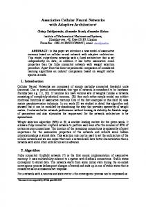
explicitly in semantic networks on the basis of views from different viewpoints and on the basis of partial views, which focus on details of the object. These views are learnt and recognised holistically by a biologically motivated neural architecture [2], [10]. Modelling on the basis of such views and partial views in an explicit representation has several advantages: (i) these views are object specific, which means that only a few objects share the same partial views; (ii) views contain information on the position and the orientation of an object in the scene, thus allowing a fast hypothesis, which can be checked by additional views; (iii) the explicit representation allows the integration of procedural knowledge on how to move the robot to certain positions to gather the necessary views. So, image acquisition is done dynamically during the evaluation of the object model. Figure 1 shows some of the images, which are taken during the recognition of a toy car. A detailed description is given in [11], [3].
Figure 1: Some characteristic views of an object
In this paper we are now concentrating on an extension of the system, that is based on the following idea. While the robot is moving from one viewpoint to another to gather characteristic views of an object, an image sequence is taken and analysed on the way. Obviously, such a sequence contains a lot of additional information. It implicitly codes the 3D structure of the object for the price of a huge amount of data. For the reduction of data and of processing time, we downsample the images in the sequence to a size of 32x32 pixels. The processing of the image sequence consists mainly of three steps: •
computing the optical flow;
•
extracting features from the flow;
•
classification of these features.
These steps will be described in detail in the following sections.
3
Selecting Feature Vectors for Recognition In any pattern recognition problem feature detection is of utmost importance. The features
extracted from different views must have a reasonable degree of invariance against shift, rotation, scale and other variations. When an object cannot be identified on the basis of information about shape, other types of information will play a critical role – motion, spatial properties (size, location), texture.
The main idea in this paper is to use motion information during a sequence of images of an object. Herein, we follow an idea of Little and Boyd [16], [17] and enhance it to 3D object recognition. It is well-known that the 3D structure of an object can be reconstructed, if a set of images and their viewing positions is given (e.g. depth reconstruction from stereo images). Therefore, the main problem to be solved is to find corresponding points in the images. The change between two images is coded by a vector (u,v) for each pair of corresponding points. Since these vectors can be used for depth reconstruction without any further information on the object, they implicitly encode the 3D structure of the object. Thus, they can be used for the identification of objects, as well. Furthermore, the identification process becomes much more robust, if based on multiple views of the object, especially in the case of ambiguous object views.
For computing the vector (u, v) for each pixel in image In compared to image In+1, we use a window-based correlation scheme as proposed by Bülthoff, Little, and Poggio [4], which is a
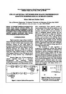
well-known technique in computer vision. Once, the vector field is given, a set of features is extracted and classified. We determine a range of scale-independent scalar features of each flow image that characterise the spatial distribution of the flow. The features are invariant to scale and do not require identification of reference points on the moving camera. The flow diagram of the system that creates our motion features is presented in Figure 2.
image sequence
optical flow
features of flow field
rearranged features of time series
Figure 2: The structure of the process for feature selection
The steps in the system are, from top to bottom: 1. The system begins with a motion sequence of n+1 images (frames) of an object.
2. The optical flow algorithm is sensitive to brightness changes caused by reflections, shadows, and changes of illumination, so we first filter the images by a Laplacian of Gaussian to reduce the additive effects. We compute the optical flow of the motion sequence to get n images (frames) of (u,v) data, where u is the x-direction flow and v is the y-direction flow. The dense optical flow is generated by minimising the sum of absolute differences between image patches. We compute the flow only in a box surrounding the object. The result is a set of moving points. Let T(u,v) be defined as: 1, if (u, v) ≥ 1 T (u, v) = 0, otherwise T(u,v) segments moving pixels from non-moving pixels. 3. For each frame of the flow, we compute a set of scalars that characterises the shape of the flow in that frame. We use all the points in the flow and analyse their spatial distribution. The shape of motion is the distribution of flow, characterised by several sets of measures of the flow. Similar to Little and Boyd [16], we compute the following scalars: •
centx :
x coordinate of centroid of moving region
•
centy :
y coordinate of the centroid of moving region
•
wcentx :
x coordinate of centroid of moving region weighted by (u,v)
•
wcenty :
y coordinate of centroid of moving region weighted by (u, v)
•
dcentx =
wcentx – centx
•
dcenty =
wcenty – centy
•
aspct :
aspect ratio of moving region
•
waspct :
aspect ratio of moving region weighted by (u,v)
•
daspct =
aspct-waspct
•
uwcentx : x coordinate of centroid of moving region weighted by u
•
uwcenty : y coordinate of centroid of moving region weighted by u
•
vwcentx : x coordinate of centroid of moving region weighted by v
•
vwcenty : y coordinate of centroid of moving region weighted by v
Each image Ij in a sequence of n images generates m=13 scalar values, sij, where i varies from 1 to m, and j from 1 to n. We rearrange the scalars to form one time series for each scalar – Si=[si1,...,sin]. These time series of scalars are then used as feature vectors for the classification step, which is implemented by using a Cellular Neural Network. Figures 3-5 show some images of a sequence and some flow images. Figure 6 visualises the feature vector of the whole sequence.
Figure 3: Some images of a sequence
Figure 4: The u component of the flow field (x-flow) visualised as normalised grey value images computed between two succeeding images of the sequence
Figure 5: The v component of the flow field (y-flow) visualised as normalised grey value images
Figure 6: Visualisation of the feature array, one column for each time series Si
It can easily be seen in Figure 6 that obviously several features are strongly correlated. Therefore, a further analysis of the features was done by evaluating correlation within the covariance matrix of the feature vectors. Thereby, we could eliminate five of the features and we concentrated our experiments on the features: centx, centy, dcentx, dcenty, aspct, daspct, vwcentx, and vwcenty.
4
Cellular Neural Networks Cellular Neural Networks (CNN) were introduced in 1988 by Chua and Yang. The most
general definition of such networks is that they are arrays of identical dynamical systems, the cells, that are only locally connected [7]. In the original Chua and Yang model each cell is a one-dimensional dynamical system. It is the basic unit of a CNN. Any cell is connected only to its neighbour cells, i.e. adjacent cells interact directly with each other. Cells not in the immediate neighbourhood have indirect effect because of the propagation effects of the dynamics of the network. The cell located in the position (i,j) of a two-dimensional N1 x N2 array is denoted by Cij, and its r-neighbourhood N rij is defined by
N rij = {Ckl | max{|k-i|,|l-j|} ≤ r; 1≤ k ≤ N1, 1≤ l ≤ N2}
(1)
Where the size of the neighbourhood r is a positive integer number.
Each cell has a state x, a constant external input u, and output y. The equivalent block diagram of a continuous time cell is shown in Figure 7. The first - order non-linear differential equation defining the dynamics of a cellular neural network can be written as follows:
C +
∂ xij (t ) ∂t
∑
C kl ∈ N
yij (t ) =
=−
1 x (t ) + R ij
∑ A (i, j; k , l ) ykl (t )
C kl ∈ N
r
ij
B (i, j; k , l ) u kl + I
r
ij
(2)
1 ( x (t ) + 1 − xij (t ) − 1 ) 2 ij
where xij is the state of cell Cij , xij(0) is the initial condition of the cell , C and R conform the integration time constant of the system , and I is an independent bias constant.
-1/R
A o u tp u ts
∫1 /C
∑
I
x ij
B
x ij( 0 )
y ij fn()
inputs
Figure 7: Block diagram of one cell. The matrices A(.) and B(.) are known as cloning templates. A(.) acts on the output of neighbouring cells and is referred to as the feedback operator. B(.) in turn affects the input control and is referred to as the control operator. Of cause, A(.) and B(.) are application dependent. A constant bias I and the cloning templates determine the transient behaviour of the cellular non-linear network. This is true. A significant feature of CNN is that it has two independent input capabilities: the generic input and the initial state of the cells. Normally they are bounded by: u ij (t ) ≤ 1
and
xij (0) ≤ 1 . Similarly, if f (.) ≤ 1
then yij (t ) ≤ 1 .
When used as an array processing device, the CNN performs a mapping
x ij (0) F ⇒ y ij (t ) u ij (t )
Where F is a function of the cloning template (A, B, I).
A two dimensional CNN can be viewed as a parallel non-linear two-dimensional filter and have already been applied in image processing problems [7], [23], [24].
A special class of two-dimensional cellular neural networks is described by ordinary differential equations of the form (see [6], [7], [18]). ∂ xij (t )
= − aij xij (t ) + ∂t yij (t) = sat (xij (t))
∑Tij, kl sat (xkl (t)) + Iij
(3)
where 1 ≤ i ≤ M, 1 ≤ j ≤ N, aij = 1/RC > 0, and xij and yij are the states and the outputs of the network, respectively. We consider zero inputs (uij ≡ 0 for all i and j) and a constant bias vector I = [I11,I12,....,IMN]T. Under these circumstances, we will refer to (3) as a zero-input nonsymmetric cellular neural network.
System (3) is a variant of the analog Hopfield model with activation function sat(.), perhaps the best known of the associative neural network memories. The Hopfield networks , in general, are completely connected. Therefore, the number of connections scales as the square of the number of units. This presents a serious problem in the VLSI implementation of large networks. This limitation has been overcome by adopting both CNN models continuous (CNNs) and discrete-time (DTCNNs) models - as associative memories [9], [19], [20], [25].
5
Design of CNNs for Associative Memories
The goal of associative memories is to store a set of desired patterns as stable memories such that a stored pattern can be retrieved when the input pattern contains sufficient information about that stored pattern.
A first attempt at developing a design method for associative memories using DTCNNs was made in [27], where the well-known Hebbian rule was used to determine the connection weights. However, serious limitations were found relating to the kind of patterns to be stored. The Hebbian training signal will not typically be optimal for learning-invariant object recognition due to erroneous classifications made by the neuron to spatially similar images from different objects and spatially dissimilar images derived from the same object.
We use the synthesis procedure presented by Liu [18] for the design of a cloning template for CNN. He considers a class of two-dimensional discrete – time cellular neural networks described by equations of the form
∂xij ∂t
= − Axij + Tsat ( xij ) + I ij (4)
yij = sat(xij) with 1≤ i ≤ m; 1≤ j ≤ n.
xij and yij are the states and outputs of the network respectively, and: A = diag[a1,...,an] T = [Tij] represents the feedback cloning template I = [I11,I12...Imn]T is the bias vector and sat(x) = [sat(x11),....,sat(xmn)]T with 1 xij ≥1 sat(xij) = 0 if −1< xij 0, i.e. choose βi = [β1i,...βni]Τ with βjiαji>1; i=1,...,m and j=1,..,n, A=diag[a1,...,an] with aj > 0 for j = 1,...,n and µ > max{ai} such that ajβji = µαji. We use A=diag[1,...,1] and µ = 10. 2. Compute the n x (m-1) matrix Y = [y1,....,ym-1] = [α1-αm,....,αm-1-αm]
(5)
3. Perform a singular value decomposition of Y = USVT, where U and V are unitary matrices and S is a diagonal matrix with the singular values of Y on its diagonal. 4. Compute T + = [Tij +] = ∑i ui (ui)T
(6)
where i=1,...,p and p = rank(Y) T - = [Tij -] = ∑i ui (ui)T
(7)
where i=p+1,...,n 5. Choose a positive value for the parameter τ and compute T = µT + - τT - and I = µαm - Tαm We use τ=0.95.
(8)
6. Then α1,....,αm will be stored as memory vectors in the system (4). The states βi corresponding to αi, i=1,...,m, will be asymptotically stable equilibrium points of system (4).
Liu also suggests a method that synthesises a sparse interconnection matrix T. There are several advantages using the eigenstructure method: 1. As is well known, the outer design method does not guarantee that every desired memory pattern will be stored as an equilibrium point (memory point) of the synthesized system when the desired patterns are not mutually orthogonal. 2. The network designed by the eigenstructure method is capable of storing equilibrium points, which by far may outnumber the order of the network. (For example of a neural network of dimension n=81 which stores 151 vector as equilibrium points, refer to [21]. 3. In a network designed by the eigenstructure method, all of the desired patterns are guaranteed to be stored as asymptotically stable equilibrium points.
System (4) is a variant of the recurrent Hopfield model with activation function sat(.) There are also several differences from the Hopfield model: 1. The Hopfield model requires that T is symmetric. We do not make this assumption for T. 2. The Hopfield model is allowed to operate asynchronously, but the present model is required to operate in a synchronous mode. 3. In a Hopfield network used as an associative memory the weights are computed by a Hebb rule correlating the prototype vectors to be stored. The connections in the Cellular Neural Network are only local. For example, a CNN of the form ( 4) with M=N=9 and r=3, has 2601 total interconnections, while a fully connected NN with n=81 will have a total of 6561 interconnections.
6
Experiments A series of experiments was done using a set of images of the Columbia image database.
This database consists of image sequences of objects, which were placed on a turntable when taking images every 5°. The background is uniform and the objects are centred. To speed up the flow computation and to handle the amount of data, we reduced the image resolution to 32x32 pixels and used only every second image. Thus, our image sequences consist of 36 low resolution images taken every 10°. The features of the image sequences of ten different objects of the database were used. Fig. 8 shows the learned objects.
Figure 8: Images of the ten objects
Fig. 9 shows an image sequence of object number two.
Figure 9: Image sequence of object number two
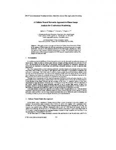
The resulting feature vectors for the time series of the feature vectors of five objects are shown in figure 10 (For completeness all 13 original features are shown). For a better visualisation they are shown as normalised grey images. We show the different features as described in sect. 3 in x-direction, the time in y-direction. One can see that they form characteristic patterns that are used for an unambiguous recognition of these objects. The associative memory is used to restore incomplete sequences and to classify them.
object 1
object 2
object 3
object 4
object 5
Figure 10: Features of five test objects shown as gray value images Obviously, recognition of a previously learnt object would not be a problem at all, since the CNN is designed such that each stored feature vector xi is an equilibrium point of the CNN.
In our experiments we wanted to measure the influence of two important parameters:
1. What happens if the object is not correctly centered in the images and 2. How sensitive is the system to noisy input images?
Thus, we modified the image sequences by translating the objects by t pixels in x- and ydirection each and by adding a random uniformly distributed noise of maximal value n to each of the images. In our test t varies from 0 to 6 and n varies from 0 to 30. Consider, that the images are only of size 32x32 pixels. Thus a translation of the object of up to 20% of the image’s size is possible. For each value of the parameters (t, n) the experiments were repeated four times – the noise was of random nature. Table 1 shows the achieved recognition rates for our test objects. Table 1: Recognition rates for varying translation and noise translation t (pixels)
noise n
recognition rate (%)
0
0
100,00
0
5
97,50
0
10
92,50
0
15
87,50
0
20
65,00
0
25
60,00
0
30
62,50
2
0
100,00
2
5
100,00
2
10
92,50
2
15
87,50
2
20
67,50
2
25
87,50
2
30
85,00
4
0
100,00
4
5
97,50
4
10
87,50
Table 1: Recognition rates for varying translation and noise translation t (pixels)
noise n
recognition rate (%)
4
15
82,50
4
20
72,50
4
25
65,00
4
30
65,00
6
0
80,00
6
5
97,50
6
10
77,50
6
15
72,50
6
20
72,50
6
25
55,00
6
30
57,50
As expected, the recognition rate decreases with increasing values of the parameters (t, n). Although there are still some outliers in the data, which have to be eliminated by larger test sets, it can be seen that a moderate amount of noise can be tolerated by the system and that a centred position of the object during the image acquisition is not required. In addition, Fig. 11 shows the average recognition rates for t