This discussion paper is/has been under review for the journal Atmospheric Chemistry and Physics (ACP). Please refer to the corresponding final paper in ACP if available.
Discussion Paper
Atmos. Chem. Phys. Discuss., 14, 22905–22938, 2014 www.atmos-chem-phys-discuss.net/14/22905/2014/ doi:10.5194/acpd-14-22905-2014 © Author(s) 2014. CC Attribution 3.0 License.
|
Jet Propulsion Laboratory, California Institute of Technology, Pasadena, California, USA 2 Joint Institute for Regional Earth System Science and Engineering, University of California, Los Angeles, California, USA 3 National Center for Atmospheric Research, Boulder, Colorado, USA 4 National Institute of Information and Communications Technology, Koganei, Tokyo, Japan
Discussion Paper
1
14, 22905–22938, 2014
Offline MLS HO2 observations L. Millán et al.
Title Page Abstract
Introduction
Conclusions
References
Tables
Figures
J
I
J
I
Back
Close
|
L. Millán1,2 , S. Wang1 , N. Livesey1 , D. Kinnison3 , H. Sagawa4 , and Y. Kasai4
Discussion Paper
Stratospheric and mesospheric HO2 observations from the Aura Microwave Limb Sounder
ACPD
Received: 18 June 2014 – Accepted: 25 August 2014 – Published: 8 September 2014 |
Full Screen / Esc
Correspondence to: L. Millán (
[email protected])
|
22905
Discussion Paper
Published by Copernicus Publications on behalf of the European Geosciences Union.
Printer-friendly Version Interactive Discussion
5
(R1)
O + XO → O2 + X
(R2)
where the net effect of these two reactions is simply, O + O3 → 2O2
(R3)
|
22906
Discussion Paper
X + O3 → XO + O2
|
Since 1985, when for the first time the now famous O3 hole was reported (Farman et al., 1985), the stratospheric O3 layer has received massive scientific attention. Although it peaks in the lower stratosphere, this layer extends well into the mesosphere where O3 chemistry is controlled by catalytic cycles involving the HOx (HO2 , OH and H) family (Brasseur and Solomon, 2005)
Discussion Paper
Introduction
ACPD 14, 22905–22938, 2014
Offline MLS HO2 observations L. Millán et al.
Title Page Abstract
Introduction
Conclusions
References
Tables
Figures
J
I
J
I
Back
Close
|
20
1
Discussion Paper
15
|
10
This study introduces stratospheric and mesospheric hydroperoxyl radical (HO2 ) estimates from the Aura Microwave Limb Sounder (MLS) using an offline retrieval (i.e. run separately from the standard MLS algorithm). This new dataset provides two daily zonal averages, one during daytime and one during nighttime, with a varying vertical resolution from about 4 km at 10 hPa to around 14 km at 0.0032 hPa. A description of the methodology and an error analysis are presented. Comparisons against the Whole Atmosphere Community Climate Model (WACCM), the Superconducting SubmillimeterWave Limb-Emission Sounder (SMILES) and the Far Infrared Spectrometer (FIRS-2) measurements, as well as, photochemical simulations demonstrate the robustness of the retrieval and indicate that the retrieval is sensitive enough to detect mesospheric HO2 layers during both day and night. This new dataset is the first long-term HO2 stratospheric and mesospheric satellite record and it provides needed constraints to help resolve the O3 deficit problem and the “HOx dilemma”.
Discussion Paper
Abstract
Full Screen / Esc Printer-friendly Version Interactive Discussion
(R4)
O(1 D) + H2 O → 2OH
(R5)
OH + O3 → O2 + HO2
(R6)
|
and, above 60 km, by photodissociation of H2 O by absorption of UV radiation (particularly in the Lyman–Alpha and the Schumann–Runge bands), H2 O + hν → OH + H
(R7)
(R8)
The removal of HOx is mainly through the self-reaction, 15
HO2 + OH → H2 O + O2
(R9)
and the partitioning between OH and HO2 above ∼ 40 km is primarily driven by, H + O3 → O2 + OH
(R11)
OH + O → O2 + H
(R12)
|
where the H produced in Reaction (R12) is quickly converted to HO2 by Reaction (R8). Despite the apparent simplicity of the HOx chemistry, models were not able to give a complete picture of the HOx chemistry in the middle atmosphere, a problem known as the HOx dilemma: Summers et al. (1997) reported that OH satellite observations by 22907
Discussion Paper
(R10)
|
20
HO2 + O → OH + O2
Discussion Paper
H + O2 + M → HO2 + M
ACPD 14, 22905–22938, 2014
Offline MLS HO2 observations L. Millán et al.
Title Page Abstract
Introduction
Conclusions
References
Tables
Figures
J
I
J
I
Back
Close
|
where H turns into HO2 due to the three body reaction
Discussion Paper
10
O3 + hν → O2 + O(1 D)
Discussion Paper
5
which destroys O3 without changing the abundance of the catalyst, X, which in this case is either OH or H. The presence of HOx family in the middle atmosphere is a consequence of the transport of H2 O and CH4 from the troposphere to higher altitudes. The production of HOx species in the middle atmosphere is primarily due to O3 photolysis
Full Screen / Esc Printer-friendly Version Interactive Discussion
22908
|
Discussion Paper | Discussion Paper
25
ACPD 14, 22905–22938, 2014
Offline MLS HO2 observations L. Millán et al.
Title Page Abstract
Introduction
Conclusions
References
Tables
Figures
J
I
J
I
Back
Close
|
20
Discussion Paper
15
|
10
Discussion Paper
5
the Middle Atmosphere High Resolution Spectrograph Investigation (MAHRSI) were 30 to 40 % lower that the values computed using standard photochemical models. Sandor et al. (1998) reported that mesospheric ground based microwave measurements of HO2 were 23 to 47 % higher than photochemical model predictions at midday, agreed with the model values prior to 9 a.m. LT, and were 70 to 100 % higher immediately after sunset. Jucks et al. (1998) using simultaneous OH and HO2 balloon observations by the Far Infrared Spectrometer (FIRS-2) reported that OH agreed reasonably well with model estimates, a conclusion supported by Pickett et al. (2008), while HO2 was 25 % higher than the model estimates. However, Canty et al. (2006) concluded that, at least between 25–60 km, the HOx Microwave Limb Sounder (MLS) and FIRS-2 observations were reasonably well described by photochemical models. Furthermore, models have consistently under-predicted the amounts of O3 at such altitudes, an issue known as the O3 deficit problem (Crutzen and Schmailzl, 1983; Solomon et al., 1983; Eluszkiewicz and Allen, 1993; Summers et al., 1997; Varandas, 2004). There have been many suggested solutions for the “HOx dilemma” and the O3 deficit problem in the literature (e.g. Miller et al., 1994; Jucks et al., 1998; Varandas, 2004); however, difficulties persist, in part, because there are very few observations of HO2 in the mesosphere. To date, there are four mesospheric datasets available: (1) six days spread between April 1992 and December 1996 measured by the Kitt Peak National Radio Astronomy Observatory (NRAO) (Sandor et al., 1998), (2) the Sub-Millimeter Radiometer (SMR) aboard the Odin satellite dataset (Baron et al., 2009), which consists of one observation period of 24 h each month between October 2003 and December 2005, (3) the Superconducting Submillimeter-Wave Limb-Emission Sounder (SMILES) ◦ ◦ dataset (Kikuchi et al., 2010), which provides daily coverage from 38 S to 65 N between October 2009 and April 2010, and (4) the standard MLS dataset (Pickett et al., 2006, 2008), which provides coverage mostly from 55◦ S to 55◦ N, up to 0.046 hPa and only during daytime. In this study, we introduce a new dataset of global observations of stratospheric and mesospheric HO2 from the MLS instrument. This new offline (i.e. run separately
Full Screen / Esc Printer-friendly Version Interactive Discussion
22909
|
| Discussion Paper
25
The Microwave Limb Sounder (MLS) is, in essence, a small radio telescope on board the Aura satellite which was launched into a polar sun-synchronous orbit in July 2004. MLS measures limb millimeter and submillimeter atmospheric thermal emission at 120 different tangent altitudes from the ground to about 95 km every 24.7 s. It cov◦ ◦ ers between 82 S and 82 N, providing near global observations with roughly half of these measurements during daytime (∼ 13:45 LT), and the other half during nighttime (∼ 1:45 LT), except near the poles where the observations transition between daytime and nighttime conditions and vice-versa. The incoming radiance is collected by a 1.6 m antenna which directs it onto four heterodyne radiometers covering spectral regions near 118, 191, 240, and 640 GHz (a fifth radiometer located at 2.5 THz is fed by a separate antenna). The radiant flux measured by the GHz radiometers is then analyzed by 22 filter banks and 4 digital autocorrelator spectrometers. Most of these filter banks were designed to measure essentially a single spectral line, despite the doubleside band nature of the radiometers (i.e. each filter bank measures two different spectral
Discussion Paper
20
ACPD 14, 22905–22938, 2014
Offline MLS HO2 observations L. Millán et al.
Title Page Abstract
Introduction
Conclusions
References
Tables
Figures
J
I
J
I
Back
Close
|
15
MLS HO2 observations
Discussion Paper
2
|
10
Discussion Paper
5
from the standard MLS algorithm) retrieval extends the HO2 vertical range well into the mesosphere (up to 0.003 hPa or ∼ 90 km), which, in addition to the standard MLS H2 O, OH and O3 , potentially allows the MLS dataset to study the HOx –O3 chemical system to provide insights for the long-standing O3 deficit problem. To date, this dataset provides almost ten years of data. In the next section we give an overview of the MLS instrument as well as the MLS HO2 measurements. Section 3 presents the offline retrieval approach and describes its vertical resolution, precision, and systematic uncertainties. Comparisons between the offline MLS HO2 dataset and global climate model simulations, balloon-borne and satellite datasets are shown in Sect. 4. Lastly, the offline HO2 data are compared to the results of a 1-D photochemical model to investigate if standard reaction rates can model the extended HO2 vertical range. Section 5 provides a summary.
Full Screen / Esc Printer-friendly Version Interactive Discussion
22910
|
Discussion Paper | Discussion Paper
25
ACPD 14, 22905–22938, 2014
Offline MLS HO2 observations L. Millán et al.
Title Page Abstract
Introduction
Conclusions
References
Tables
Figures
J
I
J
I
Back
Close
|
20
Discussion Paper
15
|
10
Discussion Paper
5
regions, one on each side of the local oscillator). Furthermore, these banks have narrower filters at the band center than at the extremes allowing them to measure the strong pressure broadening at microwave frequencies. A more detailed description of the Aura MLS instrument is given by Waters et al. (1999) and Waters et al. (2006). HO2 is measured by two of these filter banks, known as band 28 and band 30, centered at the 649.72 and 660.50 GHz HO2 lines. These filter banks consist of 11 channels with widths varying from 6 to 32 MHz, giving a total width of around 200 MHz. An example of the observed radiances is shown in Fig. 1. The ∼ 1 K HO2 signal is relatively small compared to the 2 to 4 K individual limb radiance precision, hence some averaging is required to obtain HO2 abundances with a useful signal to noise ratio. The clear tilt in band 30 is due to the proximity of an O3 line. As mentioned above, HO2 is one of the MLS products retrieved with the standard algorithm described in (Livesey et al., 2006). Briefly, the algorithm uses the optimal estimation technique (Rodgers, 2000) retrieving one profile for each scan using a twodimensional approach. The smallness of the HO2 signal translates to a retrieved product usable only between 10 and 0.046 hPa. For greater pressures, the signal is lost due to pressure broadening (i.e. Fig. 1 shows how the lines broaden rapidly as the pressure increases) and stronger emissions from O3 . For smaller pressures the signal is indecipherable from the noise. The latest version (V3.3) of the MLS HO2 standard product (Pickett et al., 2008; Livesey et al., 2011) produces ∼ 3500 abundance profiles daily with a 10◦ latitude typical precision from 0.15 ppbv (52 × 106 cm−3 ) at 10 hPa to 3 ppbv (5 × 106 cm−3 ) at 0.046 hPa. Due to the seasonality of HO2 , these values can change up to 10 % depending on the pressure level observed. Its vertical resolution varies from 4 to 10 km between 10 and 0.046 hPa. In this pressure range, since minimal HO2 is expected at night (∼ 1:45 a.m. LT for MLS at the equator), it is recommended to use the non-zero nighttime abundances as an indication of systematic biases. Hence, the HO2 day–night difference should be used as a better estimate of the daytime HO2 than taking the daytime measurements at face value. During summer and winter, this restricts the usable
Full Screen / Esc Printer-friendly Version Interactive Discussion
3
Discussion Paper |
22911
|
25
Discussion Paper
20
ACPD 14, 22905–22938, 2014
Offline MLS HO2 observations L. Millán et al.
Title Page Abstract
Introduction
Conclusions
References
Tables
Figures
J
I
J
I
Back
Close
|
15
Discussion Paper
10
For this study, an HO2 offline retrieval has been developed similar to that described by Millán et al. (2012). In essence, we compute a daily zonal mean of the radiances from which we retrieve daily HO2 concentrations. The daily zonal mean radiances are ◦ formed by collocating them into 10 latitude bins, sorting them into daytime and night◦ ◦ time using solar zenith angles (SZAs) lower than 90 and greater than 100 . Those ◦ ◦ radiances having SZAs in between 90 and 100 are disregarded to avoid twilight measurements. These sorted radiances are then interpolated onto a vertical grid of 6 surface per decade change in pressure (∼ 3 km) using the tangent pressure retrieved by the standard algorithm. The retrieval uses the optimal estimation technique as described by Rodgers (2000) assuming an HO2 a priori of zero, an a priori precision of 20 ppbv and using the corresponding daily zonal means of temperature, O3 , HNO3 , and HCl from the standard MLS algorithm (version 3.3) as part of the atmospheric state. In addition to this constraint, a Twomey–Tikhonov regularization (Tikhonov, 1963; Twomey, 1963) is used to reduce noise and smooth the profiles at the expense of some vertical resolution. The offline daytime HO2 estimates are confined to a pressure range between 10 and 0.0032 hPa with day–night differences used as a measure of daytime HO2 for pressures between 10 and 1 hPa where the nighttime values exhibit non-zero values indicative of biases. The offline nighttime HO2 estimates are confined to a pressure range between 1 and 0.0032 hPa. Figure 2 shows monthly (January 2005) zonal means for the standard and offline HO2 datasets in volume mixing ratio (VMR) and density units. The temperature used to convert the data from VMR to number density is the same zonal mean temperature from the standard MLS algorithm that is used as part of the atmospheric state. As can
|
5
Offline retrieval
Discussion Paper
HO2 standard product data to between roughly 55◦ S and 55◦ N, where MLS observes both daytime and nighttime data.
Full Screen / Esc Printer-friendly Version Interactive Discussion
Discussion Paper |
22912
Discussion Paper
The total error in the retrieved product is a combination of the random noise in the measurements, the smoothing error, and the errors due to systematic uncertainties, such as instrumental and calibration errors and forward model and retrieval approximations. Figure 4 displays the offline HO2 expected precision for daily, monthly, and yearly ◦ profiles over a 10 latitude bin. The expected precision is the error due to the combination of the random noise in the measurements and the a priori uncertainty and is given by the diagonal elements of the covariance matrix of the retrieved state (Rodgers, 2000). For a 10◦ latitude bin, for both the daytime and nighttime data, the daily HO2 precision ranges from 0.09 ppbv (29 × 106 molec cm−3 ) at 10 hPa to
|
25
Error assessment
Discussion Paper
Figure 3 shows typical averaging kernels for the HO2 offline retrieval. These kernels delimitate the region of the atmosphere from which the information is contributing to the retrieved values at a given pressure level. As such, their full width at half maximum (FWHM) is a measure of the vertical resolution. The offline HO2 product has a vertical resolution of about 4 km between 10 and 0.1 hPa, 8 km at 0.02 hPa and around 14 km for smaller pressures. The vertical resolution of this offline retrieval is similar to that of the HO2 standard product for the pressure range where they overlap. The integrated kernel shows that most of the information arises from the measurements. 3.2
20
Vertical resolution
ACPD 14, 22905–22938, 2014
Offline MLS HO2 observations L. Millán et al.
Title Page Abstract
Introduction
Conclusions
References
Tables
Figures
J
I
J
I
Back
Close
|
15
3.1
|
10
Discussion Paper
5
be seen, the offline retrieval has two distinct improvements over the standard product: (1) an extended pressure range, which enables the measurements of the mesospheric local maxima that occur at around 0.02 hPa at most latitudes, and (2) an extended latitudinal coverage, allowing to measure the polar regions, where in the summer one, the HO2 maximum lies. Furthermore, as shown in the following sections, it also estimates HO2 during night. Note that the standard MLS product is smoother because it is highly constrained due to the poor signal to noise ratio of the individual radiance profiles.
Full Screen / Esc Printer-friendly Version Interactive Discussion
Discussion Paper
22913
|
6
5
| Discussion Paper
25
Discussion Paper
20
−3
ACPD 14, 22905–22938, 2014
Offline MLS HO2 observations L. Millán et al.
Title Page Abstract
Introduction
Conclusions
References
Tables
Figures
J
I
J
I
Back
Close
|
15
6
Discussion Paper
10
−3
|
1.4 ppbv (2.2×10 molec cm ) at 0.046 hPa, and up to 7.7 ppbv (1×10 molec cm ) at 0.003 hPa. Due to the temporal variability of HO2 , these precision values can change seasonally up to 40 % depending on the pressure level observed. This variability is greater than the one found in the standard MLS product because the standard product is highly constrained due to the poor signal to noise ratio. Although significant averaging such as monthly means is needed to achieve usable HO2 estimates, this retrieval algorithm uses daily zonal mean radiances, instead of weekly or monthly, in order to enable averaging different combination of days as needed. Figure 5 summarizes the impact of the dominant systematic uncertainties for the offline MLS HO2 product. These arise from instrumental issues such as uncertainties in the radiometric calibration, the Field of View (FOV) characterization, the spectroscopy parameters, the pointing knowledge, the temperature profile used, and the retrieval approximations (a complete list and a more detailed discussion of the systematic error analysis is given by Read et al., 2007, Appendix A). The contribution of these uncertainties to the total HO2 error was estimated using end-to-end calculations. For each systematic error a full day (∼ 3500 profiles) of perturbed radiances was generated and ◦ binned into 10 zonal bins and processed by the offline algorithm. Each perturbation corresponds to either 2σ estimates of uncertainties in the relevant parameter, or an estimate of their maximum reasonable error based on instrument knowledge. Comparisons of these results with those using unperturbed radiances are a measure of the impact of each systematic error source. The comparison between the unperturbed radiances run, and the “truth” model atmosphere estimates the errors due to the retrieval numerics, which, in other words, is a measure of error due to the retrieval formulation itself. The impact of typically small error sources, such as (but not limited to) errors due to the spectrometer nonlinearities, uncertainties in the MLS spectral filter position, and the antenna transmission losses, has been quantified with a simple analytical model of the MLS measurement system (Read et al., 2007, Auxiliary material). Unlike the end-to-end estimates, these calculations only provide a multiplicative error.
Full Screen / Esc Printer-friendly Version Interactive Discussion
4.1
22914
|
| Discussion Paper
25
Figure 6 compares the MLS offline and the Far Infrared Spectrometer (FIRS-2) HO2 ◦ ◦ data. The MLS HO2 profile is a 20 latitude bin centered at 30 N averaged over 10 days centered on the day of the balloon flight. The mean SZA of this profile is ∼ 32◦ . The FIRS-2 profile shown was taken on the 20 September 2005 in Fort Sumner, New Mex◦ ico, USA (34.5 N). In that flight, the balloon stayed aloft at around 38 km for nearly 24 h. The FIRS-2 profile with the closest SZA to the MLS one is displayed, in this case ◦ ∼ 31 . FIRS-2 is a thermal emission far-infrared Fourier transform spectrometer developed at the Smithsonian Astrophysical Observatory. It measures emission spectra between 75 and 1000 cm−1 with high interferometric efficiency. It retrieves HO2 from 43 rotational transitions between 110 and 220 cm−1 (Jucks et al., 1998). The retrieval algorithm first estimates slant columns and then, in an onion-peeling fashion, a singular value decomposition routine is used to retrieve mixing ratios on a 1 km vertical grid (Johnson et al., 1996). The total systematic errors for the retrieved HO2 are estimated to be 3 %.
Discussion Paper
20
Comparison with balloon-borne instruments
|
15
Results
Discussion Paper
4
|
10
Discussion Paper
5
Between 10 and 0.1 hPa, both for the daytime and nighttime case, the total systematic error is around 0.04 ppbv (up to ∼ 10 × 106 molec cm−3 ). In this region, the main source of systematic bias arises from radiometric and spectroscopy uncertainties, in particular due to standing waves. Standing waves are a consequence of multiple reflections in the MLS optics of the hot and cold targets used as part of the radiometric calibration (Jarnot et al., 2006). For pressures smaller than 0.1 hPa, the main source of bias and scatter are retrieval numerics, which, although unsatisfactory, is understandable given the ∼ 14 km vertical resolution in this region. Around 0.0032 hPa, the total 6 −3 error is as large as 1.2 ppbv (∼ 0.2 × 10 molec cm ) .
ACPD 14, 22905–22938, 2014
Offline MLS HO2 observations L. Millán et al.
Title Page Abstract
Introduction
Conclusions
References
Tables
Figures
J
I
J
I
Back
Close
Full Screen / Esc Printer-friendly Version Interactive Discussion
22915
|
| Discussion Paper
25
Discussion Paper
20
ACPD 14, 22905–22938, 2014
Offline MLS HO2 observations L. Millán et al.
Title Page Abstract
Introduction
Conclusions
References
Tables
Figures
J
I
J
I
Back
Close
|
15
Comparisons of monthly means were made with those from the Superconducting Submillimeter Wave Limb Emission Sounder (SMILES). SMILES is a 4 K cooled radiometer on board the Japanese Experiment Module (JEM) in the International Space Station (ISS) that performed atmospheric observations from October 2009 to April 2010. It measured, on a time sharing basis, two of three frequency bands: 624.32–625.52 GHz (band A), 625.12–626.32 GHz (band B), and 649.12–650.32 GHz (band C) covering tangent heights between 10 and at least 60 km about 1600 times per day covering ◦ ◦ mostly from 65 N to 38 S. HO2 retrievals are based on radiances from band C which measures an HO2 line centered at 649.7 GHz (the same line measured by the upperside band of MLS band 28). The ISS follows a non-sun synchronized circular orbit with ◦ an inclination of 51.6 which allowed SMILES to make measurements at local times that drifted ∼ 20 min earlier each day covering the entire diurnal cycle in a period of about 2 months (Kikuchi et al., 2010). In this study we use the HO2 retrievals from the research processor (version 3.0.0) developed by NICT (National Institute of Information and Communications Technology). This version is an outcome of the latest calibrated radiances which includes an improved determination of the tangent height (e.g. Ochiai et al., 2013). These HO2 retrievals have been used for inter-satellite comparisons (Khosravi et al., 2013) and for a reaction rate estimation (Kuribayashi et al., 2014). They have a vertical resolution varying from 4 to 5 km at 35 and 55 km, respectively. The estimated precision of a single profile was estimated to be better than 30 % in the vertical range 20–86 km. In this study, only retrieval levels with a measurement
Discussion Paper
10
Satellite intercomparison
|
4.2
Discussion Paper
5
Overall, the two instruments agree on the HO2 vertical structure, with increasing HO2 with height (in the VMR representation) however there seems to be an offset between them, with the MLS data in the lower bound. Quantitatively, the MLS offline data agrees with the FIRS-2 data within their uncertainties. Result also found by Pickett et al. (2008) using the standard MLS HO2 product.
Full Screen / Esc Printer-friendly Version Interactive Discussion
| Discussion Paper
25
|
The Whole Atmosphere Community Climate Model (WACCM Version 4) is a fully interactive chemistry climate model where the radiatively active gases affect heating and cooling rates and therefore dynamics (Garcia et al., 2007). It simulates the atmosphere from the Earth’s surface to the thermosphere. For this analysis, the model was run ◦ ◦ with a horizontal resolution of 1.9 × 2.5 in latitude and longitude, and a vertical coordinate purely isobaric in the stratosphere with a variable spacing of 1.1 to 1.75 km using meteorological fields derived from the Goddard Earth Observing System 5 (GEOS-5) analyzes. The use of offline meteorological fields, a capability described by Lamarque et al. (2012), allows WACCM to perform as a chemical transport model, thus facilitating comparisons with observations. The WACCM chemical module is based on the 3-D chemical transport Model of Ozone and Related Tracers (MOZART), Version 4 (Kinni22916
Discussion Paper
20
Comparison with a global climate model
ACPD 14, 22905–22938, 2014
Offline MLS HO2 observations L. Millán et al.
Title Page Abstract
Introduction
Conclusions
References
Tables
Figures
J
I
J
I
Back
Close
|
4.3
Discussion Paper
15
|
10
Discussion Paper
5
response greater than 0.8 and lower than 1.2 have been used to avoid altitudes influenced too much by the apriori (Baron et al., 2011). Figures 7 and 8 show daytime and nighttime comparisons, respectively. Note that only SMILES measurements made within half an hour of the MLS measurements were used in this comparison. During daytime, the retrieval top level difference is as much as 80 %, however at around 0.02 hPa (the mesospheric local maxima height), the difference is overall less than ±30 %. The retrieval top level differences will need to be explored further, to investigate if they are due to retrieval artifacts (both retrievals are more sensitive to the apriori at these levels), calibration uncertainties or sampling differences. During nighttime, the overall differences are around 30 % with localized spikes due to the small nighttime values. Overall, below around 0.1 hPa these HO2 estimates agree within their uncertainties. Comparisons against SMR were not performed for two reasons: (1) the SMR mesospheric data mentioned in Sect. 1 are not publicly available and (2) SMR ascending and descending-node times are about 6.00 a.m. and 6.00 p.m., just during sunrise and sunset which complicates the comparison.
Full Screen / Esc Printer-friendly Version Interactive Discussion
22917
|
Discussion Paper | Discussion Paper
25
ACPD 14, 22905–22938, 2014
Offline MLS HO2 observations L. Millán et al.
Title Page Abstract
Introduction
Conclusions
References
Tables
Figures
J
I
J
I
Back
Close
|
20
Discussion Paper
15
|
10
Discussion Paper
5
son et al., 2007). The results of this Specified Dynamics WACCM (SD-WACCM/GEOS5) run were then sampled to the corresponding MLS observation time. Figure 9 shows a daytime monthly (January 2005) mean comparison between the offline MLS data and the SD-WACCM simulations both in VMR and density units. As can be seen, both display similar VMR structures with a strong zonal latitudinal gradient from the summer pole towards the winter pole. Note that to properly compare the data with the model simulations, Fig. 9 also shows the SD-WACCM simulations convolved with the offline MLS averaging kernels reducing the SD-WACCM high vertical resolution using a least square fit as described by Livesey et al. (2011, Sect. 1.9). In Fig. 9, the HO2 VMR peak between 0.05 and 0.01 hPa reflects the mesospheric source (Reaction R8 following Reaction R7). The zonal latitudinal gradient is a consequence of the varying SZA and the H2 O distribution, which also shows a latitudinal gradient due to the meridional circulation. The height of this peak is set by the balance between the thin air density at higher altitudes and the weakening of the UV irradiance responsible for the H2 O photolysis at lower altitudes, which leads to smaller HO2 production. In the stratosphere, as H2 O photolysis becomes less important and the H abundance decreases, HO2 mainly forms from the transformation of OH through reactions with O3 (Reaction R6). This source is reflected in the HO2 density peak in the stratosphere and has a similar shape to the peak of OH (eg., Pickett et al., 2008) but at lower altitudes due to the O3 maximum height in the lower stratosphere. Even though the offline MLS dataset and the SD-WACCM simulations display similar structures (see Fig. 9), they differ in magnitude. The offline MLS data suggest that there is more mesospheric HO2 than predicted by the model, particularly at ∼ 0.02 hPa, which requires further investigation. These differences correspond to SD-WACCM values smaller than the retrieved values by 50 % near the summer pole and smaller than 80 % near the winter pole (where SD-WACCM estimates near zero values). To investigate if these discrepancies, particularly the ∼ 4 ppbv difference at around ◦ 50 S, were due to measurement errors or due to assumptions in the SD-WACCM
Full Screen / Esc Printer-friendly Version Interactive Discussion
22918
|
Discussion Paper | Discussion Paper
25
ACPD 14, 22905–22938, 2014
Offline MLS HO2 observations L. Millán et al.
Title Page Abstract
Introduction
Conclusions
References
Tables
Figures
J
I
J
I
Back
Close
|
20
Discussion Paper
15
|
10
Discussion Paper
5
model, we compared measured MLS radiances to synthetic radiances computed using the offline MLS data and the SD-WACCM values. The SD-WACCM simulated radiances were smaller than the measured radiances by ∼ 40 %, outside the radiance error. Although MLS calibration errors cannot be ruled out, this is unlikely due to the magnitude of the offset and because this type of discrepancies cannot be found in the nighttime monthly mean comparison (Fig. 11). Hence, these simulations suggest that there is more mesospheric HO2 than modeled at around 0.02 hPa. Furthermore, as can be seen in the latitude/time cross section shown in Fig. 10, the behavior found in Fig. 9 (a 50 % difference near the summer pole and more than 80 % near the winter one) repeats itself. These discrepancies might be due to possible limitations in our current understanding of middle atmospheric chemistry and/or due to the unexpected differences between solar spectral irradiance measurements (Snow et al., 2005; Harder, 2010) and model parameterizations (Lean et al., 1997), which as pointed out by Wang et al. (2013) adds another uncertainty dimension for atmospheric modeling. In Fig. 9, between 10 and 0.1 hPa, both the offline MLS dataset and the SD-WACCM simulations, in number density units, behave in a similar manner both in structure and in magnitude; however, due to the small HO2 signal in the MLS radiances, the offline MLS retrieval is noisier. For pressure levels smaller than 0.1 hPa, the lack of a clear second peak in the SD-WACCM dataset reflects the smaller mesospheric concentrations in this dataset. Figure 11 shows the nighttime monthly mean comparison. As in the daytime comparison, both datasets show similar structures with a narrower HO2 layer in the upper mesosphere as well as a strong zonal latitudinal gradient from the summer to the winter pole. As during daytime, HO2 is principally formed through the three-body reaction of H with O2 (Reaction R8); however in this case, due to the lack of photodissociation of H2 O, the H available is the one generated at sunlit latitudes, transported at high altitudes poleward where it descends and reacts with O2 at night Pickett et al. (2006). As in daytime, despite having similar structures, both datasets differ in magnitude. Overall, the nighttime differences are smaller that the daytime differences, with SD-WACCM un-
Full Screen / Esc Printer-friendly Version Interactive Discussion
22919
|
| Discussion Paper
25
Discussion Paper
20
ACPD 14, 22905–22938, 2014
Offline MLS HO2 observations L. Millán et al.
Title Page Abstract
Introduction
Conclusions
References
Tables
Figures
J
I
J
I
Back
Close
|
15
Figure 12 shows a comparison between the HO2 estimates from MLS offline and model simulations using the Caltech/JPL-Kinetics 1-D photochemical model. This model covers from the surface to 130 km in 66 layers. It has vertical transport (including eddy, molecular and thermal diffusion) and coupled radiative transfer (Allen et al., 1981, 1984). The kinetic parameters for the calculation of rate constants and photolysis rates were specified according to JPL 2011 recommendations (Sander et al., 2011). The model was run in a diurnally varying mode with no transport until the HOx concentrations were repetitive which means a steady-state was reached. Two model runs are shown: Kinetics 1 which constrains the model using MLS measurements of H2 O, O3 , and temperature to test the HOx production and loss balance as well as the HOx partitioning and Kinetics 2 which adds a constraint to MLS OH to mostly test the HOx partitioning (Reactions R10, R11 and R12). As shown in Fig. 12, in the upper mesosphere (pressures smaller than 0.1 hPa), the Kinetics 1 simulations do not reproduce the magnitude of the measured peak, underestimating it by as much as 60 %. On the other hand, Kinetics 2 shows an improvement in the modeling of this peak, reducing the underestimation to less than 40 %. Several factors could be the reason for this discrepancy, as with the SD-WACCM model, it might be due to limitations in our current understanding of middle atmospheric chemistry and/or due to the difference between solar spectral irradiance measurements and model parameterizations. Furthermore it might be due to the low spectral resolution used in the representation of the absorption cross sections, in particular the H2 O and
Discussion Paper
10
Photochemical model comparisons
|
4.4
Discussion Paper
5
derpredicting the midlatitude summer regions by as much as 30 % and overestimating by as much as 50 % over the polar winter regions. The strong contrast, around 6 ppbv, between the daytime and the nighttime HO2 mesospheric peaks demonstrates the capability of the new offline retrieval to invert large mesospheric variations.
Full Screen / Esc Printer-friendly Version Interactive Discussion
5
Discussion Paper | Discussion Paper
25
|
We have introduced a stratospheric and mesospheric HO2 dataset derived from the Aura MLS using an offline retrieval algorithm. These offline HO2 has three distinct improvements upon the standard MLS HO2 : (1) an extend pressure range, allowing measurements of the mesospheric peak local maxima that occur at around 0.02 hPa at most latitudes, (2) an extended latitudinal coverage, which allows to measure the poles, where the HO2 maximum lies, and (3) nighttime HO2 estimates. The offline retrieval uses zonal mean MLS radiance spectra divided into daytime (SZA ≥ 90◦ ) and nighttime (SZA ≤ 100◦ ) which are then inverted using the optimal estimation technique to produce daily zonal mean HO2 profiles from 10 to 0.0032 during daytime and from 1 to 0.0032 during nighttime. The vertical resolution of this dataset is about 4 km between 10 and 0.1 hPa, 8 km at 0.02 hPa, and around 14 km for smaller pressures. Daily precision ranges from 0.1 ppbv in the upper stratosphere to up to 8 ppbv in the upper mesosphere, dropping to ∼ 1.4 ppbv and ∼ 0.5 ppbv for monthly and yearly averages, respectively. Between 10 and 0.1 hPa, for both daytime and nighttime cases, the total systematic error is around 0.04 ppbv (up to 6 −3 ∼ 10 × 10 molec cm ), while for smaller pressure levels the systematic error is as big as 1.2 ppbv (∼ 0.2 × 10⁶ molec cm−3 ). 22920
ACPD 14, 22905–22938, 2014
Offline MLS HO2 observations L. Millán et al.
Title Page Abstract
Introduction
Conclusions
References
Tables
Figures
J
I
J
I
Back
Close
|
20
Summary
Discussion Paper
15
5
|
10
Discussion Paper
1
O2 (which affects the O( D) concentration which impacts Reaction R5) cross sections, around the Lyman–Alpha region and the Schumann–Runge bands. Also, considering that Kinetics 2 (the run testing the HOx partitioning) represents the measured HO2 better, these simulations might suggest that, if there is a problem with the HO2 modeling, it is related to the HOx production and loss balance rather than the HOx partitioning. In the upper stratosphere and lower mesosphere (between 10 and 0.1 hPa) for the most part the HO2 vertical structure is simulated well in both runs suggesting that no change to the standard reactions rates is necessary, at least for those reaction rates mostly affecting those heights.
Full Screen / Esc Printer-friendly Version Interactive Discussion
Discussion Paper |
22921
|
30
Discussion Paper
25
Acknowledgements. We thank M. Allen and K. Willacy for their help with setting up and running the Caltech/JPL-Kinetics 1-D photochemical model. FIRS-2 data was funded by the NASA’s Upper Atmosphere Research program. JEM/SMILES mission is a joint project of Japan Aerospace Exploration Agency (JAXA) and National Institute of Information and Communications Technology (NICT). The WACCM modeling work was sponsored by the National Science Foundation and by the NASA Atmospheric Composition: Modeling and Analysis, solicitation NNH10ZDA001N-ACMAP. The research described in this paper was carried out by the Jet Propulsion Laboratory, California Institute of Technology, under contract with the National Aeronautics and Space Administration.
ACPD 14, 22905–22938, 2014
Offline MLS HO2 observations L. Millán et al.
Title Page Abstract
Introduction
Conclusions
References
Tables
Figures
J
I
J
I
Back
Close
|
20
Discussion Paper
15
|
10
Discussion Paper
5
Comparison with the balloon-borne FIRS-2 measurements revealed that both datasets agree within their uncertainties, however there seems to be an offset with MLS in the low side. Comparisons with SMILES were found to agree both in structure and magnitude within the uncertainties below 0.02 hPa. Qualitatively, the offline MLS HO2 agrees well with the SD-WACCM model. Quantitatively, however, the offline MLS HO2 exceeds the model by up to 100 % in the mesosphere during day (in regions where SD-WACCM estimates near zero values) and up to 40 % at night. Using the Caltech/JPL-Kinetics 1-D photochemical model we found that in the upper stratosphere and lower mesosphere the HO2 vertical structure is properly modeled using the recommended reaction rates by Sander et al. (2011). In the upper mesosphere, we found an underestimation by the model by as much as 60 % but probably in part due to the low spectral resolution of the absorption cross sections in the Lyman–Alpha region and Schumann–Runge bands. More simulations are needed to address these upper mesospheric discrepancies. The results presented in this study show that this new dataset, in addition to the standard MLS OH, H2 O, and O3 measurements, offers the possibility to study the impact of the HOx family upon the mesospheric O3 as well as the HOx dilemma. Furthermore, this retrieval, or a similar one using geomagnetic latitudes to sort the radiances, may help to understand the impact of solar proton events and energetic electron particles upon the HOx family by comparing averages of days impacted by these events with averages of non-impacted days.
Full Screen / Esc Printer-friendly Version Interactive Discussion
References
|
22922
Discussion Paper
30
|
25
Discussion Paper
20
ACPD 14, 22905–22938, 2014
Offline MLS HO2 observations L. Millán et al.
Title Page Abstract
Introduction
Conclusions
References
Tables
Figures
J
I
J
I
Back
Close
|
15
Discussion Paper
10
|
5
Allen, M., Yung, Y., and Waters, J.: Vertical transport and photochemistry in the terrestrial mesosphere and lower thermosphere (50–120 km), J. Geophys. Res., 86, 3617–3627, 1981. 22919 Allen, M., Lunine, J., and Yung, Y.: The vertical distribution of ozone in the mesosphere and lower thermosphere, J. Geophys. Res., 89, 4841–4872, 1984. 22919 Baronk, P., Dupuyk, E., Urbank, J., Urbank, D. P., Erikssonk, P., and Kasaik, Y.: HO2 measurements in the stratosphere and the mesosphere from the sub-millimetre limb sounder Odin/SMR, Int. J. Remote. Sens., 30, 4195–4208, 2009. 22908 Baron, P., Urban, J., Sagawa, H., Möller, J., Murtagh, D. P., Mendrok, J., Dupuy, E., Sato, T. O., Ochiai, S., Suzuki, K., Manabe, T., Nishibori, T., Kikuchi, K., Sato, R., Takayanagi, M., Murayama, Y., Shiotani, M., and Kasai, Y.: The Level 2 research product algorithms for the Superconducting Submillimeter-Wave Limb-Emission Sounder (SMILES), Atmos. Meas. Tech., 4, 2105–2124, doi:10.5194/amt-4-2105-2011, 2011. 22916 Brasseur, G. P. and Solomon, S.: Aeronomy of the Middle Atmosphere Chemistry and Physics of the Stratosphere and Mesosphere, 3rd revised and enlarged edn., Springer, the Netherlands, 2005. 22906 Canty, T., Pickett, H. M., Salawitch, R. J., Jucks, K. W., Traub, W. A., and Waters, J. W.: Stratospheric and mesospheric HOx : results from Aura MLS and FIRS-2, Geophys. Res. Lett., 33, L12802, doi:10.1029/2006GL025964, 2006. 22908 Crutzen, P. J. and Schmailzl, U.: Chemical budgets of the stratosphere, Planet. Space. Sci., 31, 1009–1032, doi:10.1016/0032-0633(83)90092-2 1983. 22908 Eluszkiewicz, J. and Allen, M.: A global analysis of the ozone deficit in the upper stratosphere and lower mesosphere, J. Geophys. Res., 98, 1069, doi:10.1029/92JD01912, 1993. 22908 Farman, J. C., Gardiner, B. G., and Shanklin, J. D.: Large losses of total ozone in Antartica reveal seasonal ClOx /NOx interaction, Nature, 315, 2007–2010, 1985. 22906 Garcia, R. R., Marsh, D., Kinninson, D. E., Boville, B., and Sassi, F.: Simulations of secular trends in the middle atmosphere, J. Geophys. Res., 112, D09301, doi:10.1029/2006JD007485, 2007. 22916
Discussion Paper
Copyright 2014. All rights reserved.
Full Screen / Esc Printer-friendly Version Interactive Discussion
22923
|
| Discussion Paper
30
Discussion Paper
25
ACPD 14, 22905–22938, 2014
Offline MLS HO2 observations L. Millán et al.
Title Page Abstract
Introduction
Conclusions
References
Tables
Figures
J
I
J
I
Back
Close
|
20
Discussion Paper
15
|
10
Discussion Paper
5
Harder, J. W., Thuillier, G., Richard, E. C., Brown, S. W., Lykke, K. R., Snow, M., McClintock, W. E., Fontenla, J. M., Woods, T. N., Pilewskie, P.: The SORCE SIM solar spectrum: comparison with recent observations, Sol. Phys., 263, 3–24, doi:10.1007/s11207-010-9555y, 2010. 22918 Jarnot, R. F., Perun, V. S., and Schwartz, M. J.: Radiometric and spectral performance and calibration of the GHz bands of EOS MLS, IEEE T. Geosci. Remote., 44, 1131–1143, 2006. 22914 Johnson, D. G., Orphal, J., Toon, G. C., Chance, K. V., Traub, W. A., Jucks, K. W., Guelachvili, G., and Morillon-Chapey, M.: Measurements of chlorine nitrate in the stratosphere using the ν4 and ν5 bands, Geophys. Res. Lett., 23, 1745–1748, 1996. 22914 Jucks, K. W., Johnson, D. G., Chance, K. V., and Traub, W. A.: Observations of OH, HO2 , H2 O and O3 in the upper stratosphere: implications for HOx photochemistry, Geophys. Res. Lett., 25, 3935–3938, 1998. 22908, 22914 Khosravi, M., Baron, P., Urban, J., Froidevaux, L., Jonsson, A. I., Kasai, Y., Kuribayashi, K., Mitsuda, C., Murtagh, D. P., Sagawa, H., Santee, M. L., Sato, T. O., Shiotani, M., Suzuki, M., von Clarmann, T., Walker, K. A., and Wang, S.: Diurnal variation of stratospheric and lower mesospheric HOCl, ClO and HO2 at the equator: comparison of 1-D model calculations with measurements by satellite instruments, Atmos. Chem. Phys., 13, 7587–7606, doi:10.5194/acp-13-7587-2013, 2013. 22915 Kikuchi, K., Nishibori, T., Ochiai, S., Ozeki, H., Irimajiri, Y., Kasai, Y., Koike, M., Manabe, T., Mizukoshi, K., Murayama, Y., Nagahama, T., Sano, T., Sano, R., Seta, M., Takahashi, C., Takayanagi, M., Masuko, H., Inatani, J., Susukik, M., and Shiotani, M.: Overview and early results of the Superconducting Submillimeter Wave Limb Emission Sounder (SMILES), J. Geophys. Res., 115, D23306, doi:10.1029/2010JD014379, 2010. 22908, 22915 Kinnison, D. E., Brasseur, G. P., Walters, S., Garcia, R. R., Marsh, D. R., Sassi, F., Harvey, V. L., Randall, C. E., Emmons, L., Lamarque, J. F., Hess, P., Orlando, J. J., Tie, X. X., Randel, W., Pan, L. L., Gettelman, A., Granier, C., Diehl, T., Niemeier, U., and Simmons, A. J.: Sensitivity of chemical tracers to meteorological parameters in the MOZART-3 chemical transport model, J. Geophys. Res., 112, D20302, doi:10.1029/2006JD007879, 2007. 22916 Kuribayashi, K., Sagawa, H., Lehmann, R., Sato, T. O., and Kasai, Y.: Direct estimation of the rate constant of the reaction ClO + HO2 → HOCl + O2 from SMILES atmospheric observations, Atmos. Chem. Phys., 14, 255–266, doi:10.5194/acp-14-255-2014, 2014. 22915
Full Screen / Esc Printer-friendly Version Interactive Discussion
22924
|
| Discussion Paper
30
Discussion Paper
25
ACPD 14, 22905–22938, 2014
Offline MLS HO2 observations L. Millán et al.
Title Page Abstract
Introduction
Conclusions
References
Tables
Figures
J
I
J
I
Back
Close
|
20
Discussion Paper
15
|
10
Discussion Paper
5
Lamarque, J.-F., Emmons, L. K., Hess, P. G., Kinnison, D. E., Tilmes, S., Vitt, F., Heald, C. L., Holland, E. A., Lauritzen, P. H., Neu, J., Orlando, J. J., Rasch, P. J., and Tyndall, G. K.: CAMchem: description and evaluation of interactive atmospheric chemistry in the Community Earth System Model, Geosci. Model Dev., 5, 369–411, doi:10.5194/gmd-5-369-2012, 2012. 22916 Lean, J. L., Rottman, G, J., Kyle, H. L., Woods, T, N., Hickey, J, R., Puga, L. C.: Detection and parameterization of variations in solar mid- and near-ultraviolet radiation (200–400 nm), J. Geophys. Res., 102, 29939–29956, doi:10.1029/97JD02092, 1997. 22918 Livesey, N., Snyder, W. V., Read, W. G., and Wagner, P.: Retrieval algorithms for the EOS Microwave Limb Sounder (MLS), IEEE T. Geosci. Remote., 44, 1144–1155, 2006. 22910 Livesey, N., Read, W. G., Frovideaux, L., Lambert, A., Manney, G. L., Pumphrey, H. C., Santee, M. L., Schwartz, M. J., Wang, S., Cofield, R. E., Cuddy, D. T., Fuller, R. A., Jarnot, R. F., Jiang, J. H., Knosp, B. W., Stek, P. C., Wagner, P. A., and Wu, D. L.: Earth Observing System (EOS) Aura Microwave Limb Sounder (MLS) Version 3.3 Level 2 data quality and description document, JPL D-33509, JPL publication, USA, 2011. 22910, 22917, 22928 Miller, R. L., Suits, A. G., Houston, P. L., Toumi, R., Mack, J. A., and Wodtke, J. A.: The “Ozone Deficit” Problem: O2 (X, ν ≥ 26) + O(3 P) from 226-nm Ozone Photodissociation, Science, 265, 1831–1837, 1994. 22908 Millán, L., Livesey, N., Read, W., Froidevaux, L., Kinnison, D., Harwood, R., MacKenzie, I. A., and Chipperfield, M. P.: New Aura Microwave Limb Sounder observations of BrO and implications for Bry , Atmos. Meas. Tech., 5, 1741–1751, doi:10.5194/amt-5-1741-2012, 2012 22911 Ochiai, S., Kikuchi, K., Nishibori, T., Manabe, T., Ozeki, H., Mizobuchi, S., and Irimajiri, Y.: Receiver performance of the superconducting submillimeter-wave limb-emission sounder (SMILES) on the international space station, IEEE T. Geosci. Remote., 51, 3791–3801, doi:10.1109/TGRS.2012.2227758, 2013 22915 Pickett, H. M., Read, W. G., Lee, K. K., and Lung, Y. L.: Observation of night OH in the mesosphere, Geophys. Res. Lett., 33, L19808, doi:10.1029/2006GL026910, 2006. 22908, 22918 Pickett, H. M., Drouin, B. J., Canty, T., Salawitch, R. J., Fuller, R. A., Perun, V. S., Livesey, N. J., Waters, J. W., Stachnik, R. A., Sander, S. P., Traub, W. A., Jucks, K. W., and Minschwaner, K.: Validation of Aura Microwave Limb Sounder OH and HO2 measurements, J. Geophys. Res., 113, D16S30, doi:10.1029/2007JD008775, 2008. 22908, 22910, 22915, 22917, 22928
Full Screen / Esc Printer-friendly Version Interactive Discussion
22925
|
| Discussion Paper
30
Discussion Paper
25
ACPD 14, 22905–22938, 2014
Offline MLS HO2 observations L. Millán et al.
Title Page Abstract
Introduction
Conclusions
References
Tables
Figures
J
I
J
I
Back
Close
|
20
Discussion Paper
15
|
10
Discussion Paper
5
Read, W., Lambert, A., Bacmeister, J., Cofield, R. E., Christensen, L. E., Cuddy, D. T., Daffer, W. H., Drouin, B. J., Fetzer, E., Froidevaux, L., Fuller, R., Herman, R., Jarnot, R. F., Jiang, J. H., Jiang, Y. B., Kelly, K., Knosp, B. W., Kovalenko, L. J., Livesey, N. J., Liu, H.C., Manney, G. L., Pickett, H. M., Pumphrey, H. C., Rosenlof, K. H., Sabounchi, X., Santee, M. L., Schwartz, M. J., Snyder, W. V., Stek, P. C., Su, H. S., Takacs, L. L., Thurstans, R. P., Vömel, H., Wagner, P. A., Waters, J. W., Webster, C. R., Weinstock, E. M., and Wu, D. L.: Aura microwave limb sounder upper tropospheric and lower stratospheric H2 O and relative humidity with respect to ice validation, J. Geophys. Res., 112, D24S35, doi:10.1029/2007JD008752, 2007. 22913 Rodgers, C.: Inverse Methods for Atmospheric Sounding: Theory and Practice, Vol. 2 of Series on Atmospheric, Oceanic and Planetary Physics, World Scientific, Singapore, 2000. 22910, 22911, 22912 Sander, S. P., Friedl, R. R., Barker, J. R., Golden, D. M., Burkholder, J. B., Kolb, C. E., Kurylo, M. J., Moortgat, G. K., Wine, P. H., Abbatt, J. P. D., Huie, R. E., and Orkin, V. L.: Chemical kinetics and photochemical data for use in atmospheric studies, Tech. rep., JPL, evaluation number 17, JPL Publ., 10–6, JPL publication, USA, 2011. 22919, 22921 Sandor, B. J. and Clancy, R. T.: Mesospheric HOx chemistry from diurnal microwave observations of HO2 , O3 and H2 O, J. Geophys. Res., 103, 13337–13351, 1998. 22908 Snow, M., Mcclintock, W. E., Rottman, G., Woods, T. N.: Solar–stellar irradiance comparison experiment II (Solstice II): examination of the solar–stellar comparison technique, Sol. Phys., 230, 295–324, doi:10.1007/s11207-005-8763-3, 2005 22918 Solomon, S., Rusch, D. W., Thomas, R. J., and Eckman, R. S.: Comparison of mesospheric ozone abundances measured by the Solar Mesosphere Explorer and model calculations, Geophys. Res. Lett., 10, 249, doi:10.1029/GL010i004p00249, 1983. 22908 Summers, M. E., Conway, R. R., Siskind, D. E., Stevens, M. H., Offerman, D., Riese, M., Preuse, P., Strobel, D. F., and Russell, III J. M.: Implications of satellite OH observations for middle atmospheric H2 O and ozone, Science, 227, 1967–1970, 1997. 22907, 22908 Tikhonov, S.: On the solution of incorrectly stated problems and a method of a regularization, Dokl. Acad. Nauk. SSSR, 151, 501–504, 1963. 22911 Twomey, S.: On the numerical solution of Fredholm integral equation of the first kind by the inversion of linear system produced by quadrature, J. Asss. Comput. Mach, 10, 97, 1963. 22911
Full Screen / Esc Printer-friendly Version Interactive Discussion
Discussion Paper
15
|
10
Discussion Paper
5
Discussion Paper | Discussion Paper |
22926
ACPD 14, 22905–22938, 2014
Offline MLS HO2 observations L. Millán et al.
Title Page Abstract
Introduction
Conclusions
References
Tables
Figures
J
I
J
I
Back
Close
|
Varandas, A. J. C.: Are vibrationally excited molecules a clue for the “O3 deficit problem” and “HOx dilemma” in the middle atmosphere?, J. Phys. Chem. A, 108, 758–769, 2004. 22908 Wang, S., Li, K.-F., Pongetti, T. J., Sander, S. P., Yung, Y. L., Liang, M.-C., Livesey, N., Santee, M., Harder, J., Snow, M., and Mills, F.: Midlatitude atmospheric OH response to the most recent 11-y solar cycle, P. Natl. Acad. Sci. USA, 110, 2023–2028, doi:10.1073/pnas.1117790110, 2013 22918 Waters, J., Read, W., Froidevaux, L., Jarnot, R., Cofield, R., Flower, D., Lau, G., Pickett, H., Santee, M., Wu, D., Boyles, M., Burke, J., Lay, R., Loo, M., Livesey, N., Lungu, T., Manney, G., Nakamura, L., Perun, V., Ridenoure, B., Shippony, Z., Siegel, P., Thurstans, R., Harwood, R., and Filipiak, M.: The UARS and EOS microwave limb sounder experiments, J. Atmos. Sci., 56, 194–218, 1999. 22910 Waters, J., Froidevaux, L., Harwood, R., Jarnot, R., Pickett, H., Read, W., Siegel, P., Cofield, R., Filipiak, M., Flower, D., Holden, J., Lau, G., Livesey, N., Manney, G., Pumphrey, H., Santee, M., Wu, D., Cuddy, D., Lay, R., Loo, M., Perun, V., Schwartz, M., Stek, P., Thurstans, R., Boyles, M., Chandra, S., Chavez, M., Chen, G.-S., Chudasama, B., Dodge, R., Fuller, R., Girard, M., Jiang, J., Jiang, Y., Knosp, B., LaBelle, R., Lam, J., Lee, K., Miller, D., Oswald, J., Patel, N., Pukala, D., Quintero, O., Scaff, D., Snyder, W., Tope, M., Wagner, P., and Walch, M.: The Earth Observing System Microwave Limb Sounder (EOS MLS) on the Aura satellite, IEEE T. Geosci. Remote., 44, 5, doi:10.1109/TGRS.2006.873771, 2006. 22910
Full Screen / Esc Printer-friendly Version Interactive Discussion
Discussion Paper
ACPD 14, 22905–22938, 2014
|
Offline MLS HO2 observations
Discussion Paper
L. Millán et al.
Title Page Introduction
Conclusions
References
Tables
Figures
J
I
J
I
Back
Close
|
Abstract
Discussion Paper | |
22927
Discussion Paper
Figure 1. Average MLS radiance as detected by bands 28 (top) and 30 (bottom), separated into day (solid line) and night (dashed line) time measurements. Average is from 55◦ S and 55◦ N and for limb tangents at 10 and 4.6 hPa for January 2005. The dotted gray line is the expected single scan noise.
Full Screen / Esc Printer-friendly Version Interactive Discussion
Discussion Paper
ACPD 14, 22905–22938, 2014
|
Offline MLS HO2 observations
Discussion Paper
L. Millán et al.
Title Page Introduction
Conclusions
References
Tables
Figures
J
I
J
I
Back
Close
|
Abstract
Discussion Paper | Figure 2. January 2005 zonal mean for MLS HO2 datasets. The MLS V3.3 dataset (top) is the standard product described by Pickett et al. (2008), here shown as the day–night difference as recommended by the MLS data guidelines (Livesey et al., 2011). The MLS offline (bottom) is the dataset introduced here. In this case, the day–night difference has been taken only between 10 and 1 hPa, which is the reason why this dataset can be extended to 10 hPa. The left column shows the data in VMR and the right one in number density.
Discussion Paper
22928
Full Screen / Esc
|
Printer-friendly Version Interactive Discussion
Discussion Paper
ACPD 14, 22905–22938, 2014
|
Offline MLS HO2 observations
Discussion Paper
L. Millán et al.
Title Page Introduction
Conclusions
References
Tables
Figures
J
I
J
I
Back
Close
|
Abstract
Discussion Paper Discussion Paper |
22929
|
Figure 3. Averaging kernels for the HO2 offline retrieval at the equator (those at other latitudes are very similar). The black line is the integrated area under each kernel: values near unity indicate that most information was provided by the measurements while lower values indicate that the retrieval was influenced by the a priori. The dashed gray line is a measure of the vertical resolution of the retrieved profile (derived from the FWHM of the averaging kernels approximately scaled into kilometers).
Full Screen / Esc Printer-friendly Version Interactive Discussion
Discussion Paper
ACPD 14, 22905–22938, 2014
|
Offline MLS HO2 observations
Discussion Paper
L. Millán et al.
Title Page Introduction
Conclusions
References
Tables
Figures
J
I
J
I
Back
Close
|
Abstract
Discussion Paper | Figure 4. Expected HO2 precision for a daily (D), weekly (W), monthly (M) and yearly (Y) 10◦ latitude bin. The left column shows the data in VMR and the right one in number density. The black lines show typical HO2 profiles, daytime in solid and nighttime dashed. This profile is a yearly average over all latitudes of the SD-WACCM model (see Sect. 4.3 for the model description).
Discussion Paper
22930
Full Screen / Esc
|
Printer-friendly Version Interactive Discussion
Discussion Paper
ACPD 14, 22905–22938, 2014
|
Offline MLS HO2 observations
Discussion Paper
L. Millán et al.
Title Page Introduction
Conclusions
References
Tables
Figures
J
I
J
I
Back
Close
|
Abstract
| Discussion Paper |
22931
Discussion Paper
Figure 5. Estimated impact of various families of systematic errors on the MLS offline HO2 observations. Cyan lines correspond to uncertainties in the MLS radiometric and spectral calibration. Magenta lines denote uncertainties associated with the MLS FOV and antenna transmission efficiency. Green lines denote errors in the spectroscopic databases and due to the forward model approximations. The impact of the uncertainties in the MLS pointing are depicted by the red lines. The yellow lines corresponds to errors in the retrieved MLS temperature, while the blue lines show the impact of the retrieved errors in contaminant species. Errors due to retrieval formulation are shown in gray. The black lines are the root sum squares of all the biases or the scatters shown. The top panel corresponds to the daytime part of the orbit while the lower panel corresponds to the nighttime part. The left panels show the biases and additional scatter introduced by each family of systematic errors in VMR while the right panels show them in number density.
Full Screen / Esc Printer-friendly Version Interactive Discussion
Discussion Paper
ACPD 14, 22905–22938, 2014
|
Offline MLS HO2 observations
Discussion Paper
L. Millán et al.
Title Page Introduction
Conclusions
References
Tables
Figures
J
I
J
I
Back
Close
|
Abstract
Discussion Paper |
22932
|
Discussion Paper
Figure 6. Comparison of MLS offline and FIRS-2 HO2 data from 20 September 2005 at 34.5◦ N. The MLS data correspond to the daytime–nighttime average of the 15 to the 25 September 2005 for the 20◦ latitude bin centered at 30◦ N. The MLS (gray shaded region) and FIRS-2 errors represent a combination of precision and accuracy. The left column shows the data in VMR and the right one in number density. The differences shown are FIRS-2 − MLS or (FIRS-2 − MLS) 100. / MLS (both in VMR units). The MLS averaging kernels were applied to the FIRS-2 data to fairly compare the two. The errors shown in the difference subplots corespond to the MLS and FIRS-2 errors added in quadrature.
Full Screen / Esc Printer-friendly Version Interactive Discussion
Discussion Paper
ACPD 14, 22905–22938, 2014
|
Offline MLS HO2 observations
Discussion Paper
L. Millán et al.
Title Page Introduction
Conclusions
References
Tables
Figures
J
I
J
I
Back
Close
|
Abstract
Discussion Paper |
22933
|
Discussion Paper
Figure 7. Monthly daytime zonal mean comparisons between MLS offline and SMILES HO2 data for October 2009 to April 2011. The MLS averaging kernels were applied to the SMILES data to fairly compare the two. The differences shown are SMILES − MLS or (SMILES − MLS) 100. / MLS (both in VMR units). Note that there is no HO2 SMILES data available for December 2009. As before, to alleviate biases in the MLS HO2 data, the daytime– nighttime differences are used as a measure of daytime HO2 for pressures between 10 and 1 hPa. From left to right, the datasets shown are: MLS, SMILES, SMILES with the MLS average kernels, the absolute difference and the percentage difference.
Full Screen / Esc Printer-friendly Version Interactive Discussion
Discussion Paper
ACPD 14, 22905–22938, 2014
|
Offline MLS HO2 observations
Discussion Paper
L. Millán et al.
Title Page Introduction
Conclusions
References
Tables
Figures
J
I
J
I
Back
Close
|
Abstract
Discussion Paper | |
22934
Discussion Paper
Figure 8. As for Fig. 7 but for nighttime data. Note that the large positive percentage differences shown on April 2014 close to 20◦ S and 20◦ N are due to underestimations by the MLS retrieval.
Full Screen / Esc Printer-friendly Version Interactive Discussion
SZA 30.5
32.0
62.4
72.3
SZA 30.5
32.0
62.4
0.10
70 60
1.00
50
WACCM
10.00
40
70 60
1.00
50 WACCM w MLS Av. Kernels
40
10.00
pressure [hPa]
80 0.10
70 60
1.00
50
MLS Offline -60
0 latitude 1.6
3.2
4.8
60 6.4
-60 8.0
0.0
4.0
[ppbv]
pressure [hPa]
0 latitude 8.0 6
60
12.0
-3
16.0
20.0
[10 mol cm ]
90 80 70 60 50 40
0.01 0.10 1.00 10.00 -60
[%]
Discussion Paper
0
40
ACPD 14, 22905–22938, 2014
Offline MLS HO2 observations L. Millán et al.
Title Page Abstract
Introduction
Conclusions
References
Tables
Figures
J
I
J
I
Back
Close
|
10.00
app. altitude [km]
90
0.01
Discussion Paper
pressure [hPa]
0.10
|
80
app. altitude [km]
90
0.01
app. altitude [km]
pressure [hPa]
80
app. altitude [km]
90
Discussion Paper
72.3
0.01
|
22935
|
Discussion Paper
Figure 9. January 2005 monthly daytime zonal mean for the MLS offline HO2 observations and the SD-WACCM model. To alleviate biases in the MLS HO2 data, the daytime–nighttime differences are used as a measure of daytime HO2 for pressures between 10 and 1 hPa. The MLS averaging kernels were applied to the SD-WACCM dataset to fairly compare the two. The left column shows the data in VMR and the right one in number density. From top to bottom, the datasets shown are: SD-WACCM, SD-WACCM with the MLS averaging kernels, MLS and the absolute and percentage differences. The differences shown are SD-WACCM − MLS or (SD-WACCM − MLS) 100. / MLS (both in VMR units).
Full Screen / Esc Printer-friendly Version Interactive Discussion
Discussion Paper
ACPD 14, 22905–22938, 2014
|
Offline MLS HO2 observations
Discussion Paper
L. Millán et al.
Title Page Introduction
Conclusions
References
Tables
Figures
J
I
J
I
Back
Close
|
Abstract
Discussion Paper | Figure 10. Latitude/time cross sections of the MLS offline HO2 observations and the SDWACCM model for 2005 at 0.014 hPa. As in Fig. 9, the MLS averaging kernels were applied to the SD-WACCM dataset to fairly compare the two. From top to bottom, the datasets shown are: SD-WACCM, SD-WACCM with the MLS averaging kernels, MLS and the absolute and percentage differences. The differences shown are SD-WACCM − MLS or (SD-WACCM − MLS) 100. / MLS (both in VMR units).
Discussion Paper
22936
Full Screen / Esc
|
Printer-friendly Version Interactive Discussion
SZA 149.5
148.0
109.4
117.3
SZA 149.5
148.0
109.4
0.10
70
80 0.10
70 60
WACCM w MLS Av. Kernels 1.00
0.10
70 60
MLS Offline -60 0
0 latitude 1.6
3.2
4.8
60 6.4
-60 8.0
0.0
0 latitude
0.4
[ppbv]
0.8
1.2
[106 mol cm-3]
60 1.6
2.0
0.10 -60
|
22937
60
Discussion Paper
1.00
|
90 80 70 60
0.01
app. altitude [km]
1.00
Discussion Paper
pressure [hPa]
14, 22905–22938, 2014
Offline MLS HO2 observations L. Millán et al.
Title Page Abstract
Introduction
Conclusions
References
Tables
Figures
J
I
J
I
Back
Close
|
80
app. altitude [km]
90
0.01
Discussion Paper
90
0.01
pressure [hPa]
ACPD
WACCM
1.00
pressure [hPa]
|
60
app. altitude [km]
pressure [hPa]
80
app. altitude [km]
90
0.01
Discussion Paper
117.3
Full Screen / Esc Printer-friendly Version Interactive Discussion
Discussion Paper
ACPD 14, 22905–22938, 2014
|
Offline MLS HO2 observations
Discussion Paper
L. Millán et al.
Title Page Introduction
Conclusions
References
Tables
Figures
J
I
J
I
Back
Close
|
Abstract
| Discussion Paper |
22938
Discussion Paper
Figure 12. MLS offline HO2 estimates for April 2005 and model results using JPL11 kinetics. Kinetics 1 is a photochemical model run constraining H2 O, O3 , and temperature while Kinetics 2 constrains H2 O, O3 , temperature plus OH. The differences shown are Kinetics − MLS or (Kinetics − MLS) 100. / MLS. In the difference subplots, to properly compare the model runs with MLS, a least square fit has been use to reduce the model resolution and the corresponding averaging kernels has been applied.
Full Screen / Esc Printer-friendly Version Interactive Discussion