Journal of Mechanical Science and Technology 25 (12) (2011) 3115~3121 www.springerlink.com/content/1738-494x
DOI 10.1007/s12206-011-1219-9
On a component mode synthesis on multi-level and its application to dynamics analysis of vehicle system supported with spring-stiffness damper system† Seongsoo Lee1, Hyungsoo Mok2 and Chang-Wan Kim1,* 1
School of Mechanical Engineering, Konkuk University, Seoul 143-701, Korea Department of Electrical Engineering, Konkuk University, Seoul 143-701, Korea
2
(Manuscript Received January 10, 2011; Revised April 3, 2011; Accepted July 12, 2011) ----------------------------------------------------------------------------------------------------------------------------------------------------------------------------------------------------------------------------------------------------------------------------------------------
Abstract The component mode synthesis (CMS) method on multi-level, called as recursive component mode synthesis (RCMS) method, is implemented for the free vibration analysis of a vehicle system supported on damper-controlled spring-stiffness suspension. The nonproportional damping is considered to describe the suspension system. The focus of the RCMS method is the out-of-core concept that uses disk space rather than memory when computing large scale vehicle FE models. After the eigensolutions are obtained, the mode superposition method is used to compute the dynamic response in the frequency domain. The proposed method can deal with a damped structural system with a general damping system. The performance and accuracy of the proposed method compared to the Lanczos method are demonstrated through an example FE model. Keywords: NVH; Component mode method; Non-proportional damping; Frequency response; Out-of-core concept ----------------------------------------------------------------------------------------------------------------------------------------------------------------------------------------------------------------------------------------------------------------------------------------------
1. Introduction The automotive industry has pursued the design of a vehicle that rides comfortly and quietly. Recently, there has been growing concern that analysts continue to increase the excitation frequency range of noise, vibration, and harshness (NVH) analysis. Subsequently, the size of the finite element (FE) model for NVH analysis also grows. Although the automobile industry increasingly invests in high performance computer hardware, there are still limitations in computer resources such as CPU, memory, I/O, and storage to satisfy NVH analysis demands. One of the essential parts of NVH analysis is to obtain the natural frequency through the free vibration analysis. For large scale structures in industry, the most conventional approach to calculate the eigenvalues and the corresponding eigenvectors is to use the Lanczos method [2]. The Lanczos method is recognized as a powerful tool for extracting partial eigensolutions in large scale structural dynamics. However, for large scale FE models, the major difficulty of the Lanczos method is the significant amount of disk space, memory, and I/O requirements [1]. Therefore, industries have been motivated to develop a method that can reduce computational costs while obtaining †
This paper was recommended for publication in revised form by Editor Maenghyo Cho Corresponding author. Tel.: +82 2 450 3543, Fax.: +82 2 447 5886 E-mail address:
[email protected] © KSME & Springer 2011 *
sufficient accuracy for computing eigensolutions. Several new developments have been emerging for efficient computation of eigenvalue problem. Component mode synthesis (CMS) method has been most widely used over past three decades in industries [3-5]. CMS methods are substructuring techniques frequently employed in structural dynamics. A given analysis model is subdivided into components or substructures which are analyzed independently for natural frequencies and mode shapes. The substructure mode shapes are then assembled to compute natural frequencies and mode shapes of the original structural system. Although the CMS method is suitable for eigenanalysis of large scale structures, several researchers showed that the implementation of the CMS method on multi-level will be more adequate for extremely large scale eigenanalysis than the conventional one. The implementation of CMS method or substructuring method on multi-level has been attempted [815] as a generalization of the classical CMS method. Since most of researches used in-core approach, which uses a computer’s main memory in numerical implementation, it is strongly required to use out-of-core approach in order to solve practical large scale industry applications. Out-of-core or external memory algorithms are algorithms that are designed to process data that is too large to fit into a computer’s main memory at one time. Such algorithms must be optimized to efficiently fetch and access data stored in slow bulk memory such as hard disk.
3116
S. Lee et al. / Journal of Mechanical Science and Technology 25 (12) (2011) 3115~3121
Fig. 2. A single level domain partitioning.
Fig. 1. Damper controlled spring-stiffness suspension system.
order n can be represented by (1)
So far, various types of above CMS research works are confined only to the eigenvalue problem analysis. Therefore, it is also strongly motivated to extend the CMS method on multi-level to the dynamic response analysis in the frequency domain [16, 17], especially including nonproportional damping. In this paper, the CMS on multi-level with out-of-core algorithm is applied to the mode superposition method. The problem of interest in this paper is a large vehicle system supported on damper controlled spring-stiffness suspension as shown in Fig. 1. To describe the suspension system, non-proportional dampings [17, 18], structural and viscous damping, should be considered. In particular, in order to consider large scale industry automobile FE models that require a large amount of disk space and memory, this paper also describes an out-ofcore algorithm for the multi-level CMS method, which uses disk space rather than memory in computation. In a numerical example, the amount of data transferred between disk and memory and the maximum disk usage are measured compared with those of the Lanczos method, which is also out-of-core. Also, the performance and accuracy of the proposed method compared to the Lanczos method are validated.
2. Free vibration with the CMS method on multi-level The main cost in computing the dynamic response in the frequency domain is to compute the eigenvalue problem of the pencil (K,M), where K and M are the FE stiffness and mass matrices, and solve the modal frequency response problem with the computed eigensolutions. This section describes the CMS method on multi-level with out-of-core to compute the eigenvalue problem, up to a cutoff frequency of FE models. 2.1 A single level CMS method The main steps of the CMS method are four steps: (1) form the global equations of motion, (2) partition an FE model into many components, (3) reduce the model using the transformation matrix, and (4) compute the reduced eigenvalue problem. In the first step, the eigenvalue analysis of the FE model of
where [K] are [M] ∈ R n×n the FE stiffness and mass matrices, respectively. λ is the eigenvalue, and {u} ∈ R n×n is the corresponding eigenvector. Next, an FE model is partitioned into several components. Fig. 2 illustrates that a FE model is divided into component S1 and S2, in which component S3 is an interface between component S1 and S2. Then, Eq. (1) is reordered as:
(2) where the subscript 1 and 2 represent a set of local degrees of freedom for component S1 and S2, which are in the interior of the partitioned domain, and the subscript 3 represents a set of shared degrees of freedom, which are in the interface of the partitioned domain. The dimension of the local degrees of freedom is n1 and n2 for the component 1 and 2, and n3 for the component 3, in which n = n1 + n2 + n3. In the third step, a transformation matrix should be obtained to form the reduced matrices, based on the Craig and Bampton method [4]. A transformation matrix [T] is constructed from the product of each component transformation matrix as [12].
(3) where [T1] and [T2] are the transformation matrices for the component 1 and 2, respectively. The −K11−1 K13 and − K −221 K 23 are constraint modes, which are the static boundary transformation between the interior and interface degrees of freedom. The fixed interface normal modes Φ1 and Φ 2 for the interior degrees of freedom are obtained from the following eigenvalue problem:
S. Lee et al. / Journal of Mechanical Science and Technology 25 (12) (2011) 3115~3121
3117
(4) (5) (a)
where Λ1 and Λ 2 are the eigenvalue matrices, Φ1 and Φ 2 are the corresponding eigenvector matrices. Because the transformation matrix [T] contains only partial eigenvectors of Φ1 and Φ 2 , up to a cutoff frequency, the number of columns s of [T] is less than n because most structure engineers are interested mainly in finding lower frequency modes that are important to understand structural characteristics. Using the transformation matrix [T] ∈ R n×s , the reduced mass and stiffness matrices, [M] ∈ R s×s and [K ] ∈ R s×s , can be obtained as:
(b)
(6)
(c)
(7) where (8) (9)
. (10) As a final step, the reduce eigenvalue problem of the pencil (K,M) is solved to obtain the approximate eigensolution of the pencil (K,M) . 2.2 Multi-level CMS method A traditional CMS method, which is on a single level, can be extended to a multilevel algorithm naturally by partitioning a FE model into several smaller components on multi-level. Note that all component matrices are stored on hard disk for the out-of-core algorithm, and only a few component matrices are called into memory whenever they are needed for computation. Fig. 3 illustrates a FE beam model partitioning procedure. First, the FE model is divided into two interior components, S7 and S14, and the interface component S15. Then, the component S7 is divided again into components S3 and S6. Similarly, the component S14 is partitioned into S10 and S13. The parti-
(d) Fig. 3. Tree topology: (a) FE model; (b) level 1; (c) level 2; (d) level 3.
tioning is continued up to the three levels tree as shown in Fig. 3(d). Fig. 4 shows the pattern of the reordered mass and stiffness matrices based on the three level tree partitioning. Once the matrices are partitioned and reordered, we can compute the transformation matrix [Ti] for each component, Si(i = 1, …, ncm), where ncm is the number of components. Based on the single level CMS method, the general form of transformation matrix [TL] for the component L can be represented as:
(11) where Φ L is the fixed interface normal mode for the local degrees of freedom set, K LL Φ L = M LL Φ L Λ L .
3118
S. Lee et al. / Journal of Mechanical Science and Technology 25 (12) (2011) 3115~3121
Fig. 4. Reordered matrix pattern.
Kim [12] proposed the transformation matrix [Tncm] for the last component Sncm, S15 in Fig. 3. The [Tncm] includes only the fixed interface normal mode Φ ncm in order to diagonalize the transformed stiffness matrix. Without [Tncm], the transformed component stiffness and mass matrices for the last component Sncm remain block matrices on diagonal as shown in Eqs. (6) and (7). Then, the transformation matrix [T] ∈ R n×s for the entire structure is the product of all component transformation ncm [Ti ] . Note that s is much smaller matrices, [T] = [T] = ∏i=1 than n because only partial eigenvectors of Φ L , (L = 1, …, ncm) are kept in the transformation matrix [T]. The transformation for [K] and [M] matrices is preceded from the bottom level components to the top component as [12].
(12) (13) In the out-of core approach, the required memory usage during the transformation related to component Si is only for the non-zero blocks of the corresponding transformation matrix [Ti] and some component matrices, Ki,j and Mi,j , to be multiplied by the non-zero blocks of [Ti]. For example, the transformation matrix [T1] for the component S1 has non-zero entries only in the first row except an identity on the diagonal for other rows. The entries of the first row are (14) in which T1,1 is the fixed interface normal mode Φ1 , and T1,k = -K11−1 K1k , k=3, 7, 14 are the constraint mode. In the transformation procedure for the component S1, [T1]T[K][T1], the required memory usage is only for T1,1, T1,3, T1,7, and T1,14 entries in [T1], and the component matrices Ki,j and Mi,j for i, j =1, 3, 7, 15. Generally, each component transformation matrix [Ti] is very sparse, so that only a small amount of memory is required during the matrix transformation in the out-of-core
approach. In addition, the data I/O transferred between memory and disk is not significant for the same reason. These advantages result in an efficient out-of-core algorithm for the CMS method on multi-level. However, the Lanczos method, which is one of the most popular methods for large scale eigenvalue problem, requires a significant amount of data I/O and disk usage because it deals with the whole finite element matrices and keeps the many Lanczos vectors during the Lanczos iterations [1]. Once the transformed stiffness matrix, which is a diagonal matrix containing only component eigenvalues below the component cutoff frequency, and the transformed mass matrix, which has an identity matrix on the diagonal and some block dense matrix off the diagonal, are obtained [12], the following generalized eigenvalue problem for the reduced system is solved: .
(15)
Because the stiffness matrix [K] is reduced to a diagonal matrix [K], it is trivial to transform the generalized eigenvalue problem in Eq. (15) to the standard eigenvalue problem as: (16) where the eigenvector { ur } ∈ R S approximates the FE space eigenvector as {u} ≈ [T ]{ur}, and the approximate eigenvalue for FE space is λ ≈ λr . For out-of-core algorithm, the transformation matrices [T] is stored in disk in order to approximate FE eigenvector {u} ≈ [T ]{ur}. The accuracy of the CMS method is typically lower than the Lanczos method; however the level of accuracy can be accepted for the frequency response problem related to the NVH engineering application. The accuracy depends on how to select eigenvectors from each component.
3. Modal frequency response analysis After the eigenvalue analysis is finished, the dynamic response computation continues with the modal frequency response analysis, or mode superposition method In an automobile structure, a suspension system, illustrated in Fig. 1, not only makes the ride more comfortable, but also maintains better control in severe off-road riding. Damping should be applied to slow down the spring action. In particular, the nonproportional damping [19] is essential to describe the suspension system. Damping generally uses oil or air, for which viscous damping should be applied. Structural damping considers the use of internal friction in a material to dissipate vibrational energy into heat. For a given displacement x(t) and velocity ɺ x(t) with structural damping, the resulting forces are in the form [1, 18] .
(17)
3119
S. Lee et al. / Journal of Mechanical Science and Technology 25 (12) (2011) 3115~3121
Table 1. The number of nodes and elements of finite element model.
The viscous damping force is represented as: .
(18)
Nodes
1-D element
2-D element
3-D element
317,061
39,268
266,047
9,043
The scalar γ is a global structural damping coefficient and i = −1 . [B] and [Ks] are the FE viscous damping matrix and the local structural damping matrix, respectively. Generally, [B] and [Ks] are called as non-proportional damping [18]. Generally, vehicle ride performance is evaluated with the examination of frequency responses. Designers focus on the maximum magnitude of responses at specific locations such as passenger seat and steering locations, and wheels. In order to examine frequency responses, a system of equations for the direct frequency response analysis [1] with non-proportional damping in the FE dimension of order n can be formulated as: . (19) Then, with the mode superposition method [18], the Eq. (19) is projected onto the modal space by substituting X(ω)= [Φ]Z(ω) into Eq. (19) and pre-multiplying Eq. (19) by [Φ]T. Note that [Φ] ∈ R n× m is obtained from [Φ] ≈ [T ][Φr], in which [Φr] = {ur,1, ur,2, …, ur,m} ∈ R s×m is obtained from Eq. (16) and m is the number of modes obtained below the cut off frequency. It results in the following equation: . (20) With the orthogonality relationships and mass normalization, [Φ]T [M ][Φ] = [I] and [Φ]T [M ][Φ] = [Λ] ∈ R m×m , the modal non-proportional damping matrices are defined as [ B ] = [Φ]T [B ][Φ] and [ K S ] = [Φ]T [KS ][Φ] ∈ R m×m , and F(ω) = [Φ]T P(ω) ∈ R m . Once the modal solution Z(ω) is obtained over the desired excitation frequency range, the modal solutions is back transformed to get the frequency response in the FE dimension as: .
(21)
4. Forced vibration analysis of vehicle system supported with damper suspension 4.1 Vehicle FE model description In order to evaluate the performance and transferred data I/O amount of the RCMS method, a passenger automobile FE model supported on damper controlled spring-stiffness suspension is used as a numerical example. This car model has all the major components of a car, such as wheels, engine, and suspensions. Commercial finite element software NASTRAN [21] is used for the finite element model. Table 1 shows the number of nodes and elements of the FE model. Since automobile FE model is company proprietary and confidential information, the detail information of FE model is not permit-
Fig. 5. Tree topology of the finite element model with 2,284 components.
ted to be published. One-dimensional elements include bar, elastic, and rigid elements. Triangular and quadrilateral elements are used for two-dimensional elements, and a hexagonal element is used for three-dimensional elements. The total number of nodes is 317,061, and the degrees of freedom are 1,902,366. Discrete damping elements such as CBUSH, CVISC, CDAMP elements describe the suspension system. Also, structural damping coefficients are included in finite element properties for the suspension system. 4.2 Accuracy and performance evaluation The performance, transferred data I/O amount and accuracy of the RCMS method are compared with the Lanczos method. HP-UX B.11.22 Itanium 2 with 4 Gb RAM and 200 GB disk workstation is used for evaluating the performance of the RCMS method. In this paper, the Lanczos algorithm in NASTRAN [21] is used. The RCMS uses the FE matrices obtained from NASTRAN, so both the RCMS and the Lanczos algorithm use the same FE matrices in the computation. Note that the Lanczos method deals with the FE matrices of order n directly, while the RCMS method considers the reduced matrices of order s. First, the METIS software [20], which is a well known graph partitioner, is used for partitioning finite element matrices. Fig. 5 illustrates the tree topology that has 25 levels with 2,284 components. Then, the partial eigensolutions are computed based on the tree topology. Two different partial eigensolutions are obtained with different cutoff frequencies, 150 Hz and 300 Hz. For the cutoff frequency 150 Hz, The structure is excited from 1 Hz to 100 Hz. After the FE matrices are transformed, the dimensions of the reduced matrices in Eq. (6) becomes 7,587. Both the RCMS method and the Lanczos method compute 505 global modes including 6 rigid body modes. With 300 Hz cutoff frequency, the reduced matrices of 18,998 rows and columns
3120
S. Lee et al. / Journal of Mechanical Science and Technology 25 (12) (2011) 3115~3121
Table 2. The comparison of elapsed time (hh:mm:ss) for eigenvalue analysis with different cutoff frequency.
Table 4. The disk I/O transferred for 300 Hz cutoff frequency.
150 Hz
37:42
3:31:59
RCMS method
20.2 GB
Total disk I/O transferred 177 GB
300 Hz
1:39:26
11:54:05
Lanczos method
64.8 GB
4,603 GB
Cutoff frequency
RCMS method
Lanczos method
Eigenvalue analysis
Maximum disk usage
Table 3. The detailed elapsed time (hh:mm:ss) of dynamic response analysis with the RCMS method. Cutoff frequency
150 Hz
300 Hz 1:13:17
Transformation for [K] and [M]
35:11
Eigenvalue analysis [K]{ur} = λr [M]{ur}
2:31
26:09
Modal frequency response analysis
1:11
17:48
Total time
38:53
1:57:14
(a) Point 2
Fig. 6. Relative percent error of eigenvalues obtained from the RCMS method and the Lanczos method.
are obtained after the transformation on multi-level, in which the structure is excited from 1 Hz to 200 Hz. Both the RCMS method and the Lanczos method provide 1,517 global modes. In computing the partial eigensolution, the performance of the RCMS and the Lanczos method is presented in Table 2. For each cutoff frequency, the RCMS method is about 5.5 and 6.1 times faster than the Lanczos method. In the modal frequency response analysis, both the RCMS and the Lanczos method give the same performance because the dimension, not entries, of modal matrices are the same due to the same number of global modes. For each cutoff frequency, Table 3 compares the elapsed time of each step with the RCMS method: transformation in Eqs. (12) and (13), eigenvalue analysis in Eq. (15), and modal frequency response analysis in Eq. (20). Most of the computational time is spent on the transformation process, 91 and 62 percent of total time, for each cutoff frequency. Fig. 6 shows the relative error between the eigenvalues from the RCMS method and the Lanczos method for the cutoff frequency 300 Hz. The relative error of eigenvalues increases as the natural frequency increases, but the maximum relative error is only 0.61%. It shows that the eigenvalues obtained with the RCMS method are good approximations to those of the Lanczos method. The main focus of this application paper is the maximum
(b) Point 2 Fig. 7. Comparison of frequency responses up to 200 Hz for two different locations from the RCMS method and the Lanczos method.
disk usage and total disk I/O transferred, which is represented in Table 4. With the RCMS method, the maximum amount of disk space is decreased 68:8%, and the total disk I/O transferred is decreased 96:2% compared to the Lanczos method. This is because the RCMS method deals with only the nonzero blocks of FE matrices and transformation matrices, as explained in the previous section. In addition, the RCMS method considers the reduced matrices instead of the global finite element matrices that the Lanczos method uses. The Lanczos method requires especially large amount of disk space to keep many Lanczos vectors until the analysis is finished. Also, it requires large amount of disk I/O during the Lanczos iterations [1]. The frequency responses in Fig. 7 illustrate the magnitude of acceleration for two different locations. The responses from the RCMS method represent approximation to the responses from the Lanczos method, which provide very good approxi-
S. Lee et al. / Journal of Mechanical Science and Technology 25 (12) (2011) 3115~3121
mations in this case. This means that the eigensolution of the RCMS method is accurate enough to represent the frequency response, which is almost the same as the frequency response obtained from the Lanczos method.
5. Conclusions This case study paper presents the application of the RCMS method, which is designed for out-of-core, to the NVH analysis of a large vehicle system supported on damper-controlled spring-stiffness suspension. The non-proportional damping, structural and viscous damping, are used to describe the vehicle suspension system. For a large scale vehicle system, the RCMS method with out-of-core reduces computational costs significantly while obtaining sufficient accuracy compared to the Lanczos method. It results in good frequency response approximation. In addition, the amounts of data transferred between disk and memory, and the disk usage are greatly reduced compared with the Lanczos method. Therefore, by saving computational time as well as computational resources such as disk space for automobile engineers, resulting in shorter design cycle, the RCMS method can be an efficient tool for the NVH analysis of large scale automobile structures.
Acknowledgment This research was supported by Basic Science Research Program through the National Research Foundation of Korea (NRF) funded by the Ministry of Education, Science and Technology (grant number 2009-0077217, 2009-0067895 and 2010-00525).
References [1] MD/MSC Nastran 2010, Numerical methods user’s guide, MSC.software cooperation, USA (2010). [2] Louis Komzik the Lanczos method: Evolution and application, SIAM (2003). [3] W. C. Hurty, Vibration of structural system by component mode synthesis, ACES Journal of the Engineering Mechanics Division (1960) 86, no. EM4, 51-69. [4] R. R. Craig and M. C. Bampton, Coupling of substructures for dynamic analysis, AIAA Journal, 6 (1968) 1313-1319. [5] L. Meirovitch and A. L. Hale, On the substructure synthesis method, AIAA Journal, 19 (1981) 940-947. [6] I. Takewaki and K. Uetani, Inverse component-mode synthesis method for damped large structural systems, Computers&Structures (2000) 78 (1-3) 415-423. [7] Y. Aoyama and G. Yagawa, Component mode synthesis for large-scale structural eigenanalysis, Computers & Structures (2001) 79 (6) 605-615. [8] J. K. Bennighof, M. F. Kaplan, M. Kim, C. W. Kim and M. B. Muller, Implementing automated multi-level substructuring in nastran vibroacoustic analysis, Proc. of SAE Noise and
3121
Vibration Conference, SAE paper (2001) 01-1405. [9] K. Elssel and H. Voss, Multilevel extended algorithms in structural dynamics on parallel computers, Proc. of PARCO2003, Dresden, North-Holland (2004). [10] U. L. Hetmaniuk and R. B. Lehoucq, Multilevel methods for eigenspace computations in structural dynamics, Proc. of 16 th International Conference, Domain Decomposition Mehtods, New York, January (2005). [11] C. Yang, W. G. Gao, Z. Bai, X. Li, L. Lee, P. Husbands and E. G. Ng, An algebraic sub-structuring algorithm for large-scale eigenvalue calculation, SIAM J. Sci. Comp. 27 (3) (2005) 873-892. [12] C. W. Kim, Analysis of vibration levels of large structural system with re-cursive component mode synthesis method: Theory and convergence, ProcInstn MEch Engrs Part C: J. of Mechanical Engineering Science, 220 (9) (2006) 13391345. [13] J. H. Ko, D. Byun and J. S. Han, An efficient numerical solution for frequency response function of micromechanical resonator arrays, The Journal of Mechanical Science and Technology, 23 (10) (2009) 2694-2702. [14] D. Choi, H. Kim and M. Cho, Iterative method for dynamic condensation combined with substructuring scheme, Journal of Sound and Vibration (2008) 317 (1-2) 199-218. [15] H. Kim and M. Cho, Improvement of reduction method combined with sub-domain scheme in large-scale problem, International Journal for Numerical Methods in Engineering (2006) 72 (2) 206-251. [16] J. H. Ko and Z. Bai, High frequency response analysis via algebraic sub-structuring, International Journal of Numerical Method in Engineering, 76 (3) (2008) 295-313. [17] C. W. Kim, Efficient modal frequency response analysis of large structures with structural Damping, AIAA Journal, Gatlinburg, Tennessee, 44 (9) (2006) 2130-2133. [18] L. Meirovitch, Principles and techniques of vibrations, Prentice Hall (1997). [19] C. W. Kim, Fast frequency response analysis of large-scale structures with non-proportional damping, International Journal for Numerical Methods in Engineering, 69 (5) (2007) 978-992. [20] G. Karypis and V. Kumar, METIS: A software package for partitioning unstructured graph, partitioniing Meshes, and computing fill-reducing orderings of sparse matrices, version 4.0 University of Minnesota, MN, USA (1998). [21] MD/MSC Nastran 2010, Release Guide, MSC.software cooperation, USA (2010).
Chang-Wan Kim received B. S. degree in Hanyang Universty, M.S. degree in POSTECH, and Ph.D from the University of Texas at Austin, USA. His research interests are computational design and analysis. Recently, multi-physics analysis with CAE on mechanical system is main research topic.