On a Local Maximum Entropy interpolation

Thèse de Doctorat

Mathieu FOCA Mémoire présenté en vue de l’obtention du grade de Docteur de l’École Centrale de Nantes sous le label de l’Université Nantes Angers Le Mans École doctorale: Sciences pour l’Ingénieur, Géosciences, Architecture (SPIGA) Discipline: Mécanique des solides, des matériaux, des structures et des surfaces Unité de recherche: institut de recherches en Génie civil et Mécanique (GeM) Soutenue le vendredi 16 janvier 2015

On a Local Maximum Entropy interpolation approach for simulation of coupled thermo-mechanical problems. Application to the Rotary Frictional Welding process. JURY Président:

Pierre VILLON, Professeur des Universités, UTC de Compiègne

Rapporteurs:

Ignacio ROMERO, Professeur, Université Polytechnique de Madrid Eric FEULVARCH, Maître de conférence HDR, ENI de Saint-Étienne

Examinateurs:

Elias CUETO, Professeur, Université de Zaragoza Jean-Philippe PONTHOT, Professeur, Université de Liège

Directeur de thèse: Co-Directeur de thèse:

Laurent STAINIER, Professeur des Universités, École Centrale de Nantes Guillaume RACINEUX, Professeur des Universités, École Centrale de Nantes

Ces trois années et demi passées au GeM comptent à ce jour parmi les plus belles années de ma vie, riches en événements, en rencontres et, bien évidemment, riches d'un point de vue scientique. Je tiens tout d'abord à remercier l'ensemble des membres de mon jury pour avoir eu la gentillesse de m'accorder un peu de leur temps en ces périodes de n et de début d'année : Pierre Villon, qui m'a fait l'honneur de présider ce jury ; Ignacio Romero et Eric Feulvarch, pour leur relecture attentive et minutieuse, leur regard critique et leurs commentaires constructifs ; Jean-Philippe Ponthot pour ses questions judicieuses lors de la soutenance et enn Elias Cueto pour son suivi tout au long de mes années de thèse. Je remercie également Patrick Romilly, invité, pour avoir suivi ce projet en y apportant la dimension industrielle permettant de toujours avoir en vue la raison de nos recherches parfois si abstraites. J'adresse de sincères remerciements à mon directeur de thèse, Laurent Stainier, non seulement pour m'avoir accordé sa conance sur ce sujet passionnant mais aussi pour m'avoir permis d'aller littéralement à l'autre bout du monde. Je tiens également à témoigner toute ma reconnaissance à mon co-encadrant de thèse, Guillaume Racineux, pour sa grande gentillesse et ses conseils pratiques et avisés. Un grand merci à toute l'équipe de l'équipe Structure et Simulation : Nicolas M., Claude et Antony pour leurs questions toutes plus redoutées les unes que les autres en réunion d'équipe mais également les plus pertinentes ; Eric et Pierre-Emmanuel pour leur grande patience vis-à-vis de mes talents avec Linux; Gregory, Laurent G., Nicolas C., Pascal, Patrice et Patrick avec qui c'est toujours un plaisir de discuter et ce depuis mes années en cycle ingénieur ; et tous les autres pour leur gentillesse, Caroline, Marie, Mélissa, Alexis, Gilles et Thomas. Une petite pensée pour tous ceux avec qui j'ai eu la chance de partager mon bureau : les grands anciens Shaopu, JC et Augusto (même si à l'arrivée seule la demoiselle a soutenue avant moi !), celle qui n'a fait qu'y passer Qian et les petits derniers Daria et, bien évidemment, mon grand ami Simon ! Un gros clin d'÷il à tous les collègues et amis pas encore cités : ce petit lou de Romain, perspicace et inquiétant ; Loïc, dit Lolo d'Arabie, mon partenaire de muscu ; Kévin qui m'a tout appris ; Ophélie la machine inarrêtable ; Prashant le californien ; Matthieu et Andrès, indisociables et toujours en train de se sacrier/d'être sacriés pour que tout se déroule pour le mieux ; et tous les autres: Alina, Elia, Florent, Benoît, Bérenger, Cyril, Quentin et Olivier. Évidemment je me dois d'avoir une pensée pour le groupe nantais des 6trouilles dont les soirées jeux et Magic ont rythmé ces années de thèse : Gaël, Simon, TT et Mélanie, Thibault, Xavier, Denis, Fred, Octavio, Antonin et Élodie, Manu et Mady. Une pensée également pour mes amis toulousains: Gurb, Geb le moche, Geb le geek, JTM, Poulpy et Julien. Enn, je tiens à remercier chaleureusement ma famille : Papa et Maman pour leur présence le jour de ma soutenance et leur soutien inconditionnel durant toutes ces années. Je ne saurais nir sans une douce pensée pour ma chère Marie, qui m'a toujours soutenue et qui me supporte depuis toutes ces années.

Contents

Contents

i

List of Figures

v

List of Tables

vii

1 Introduction 1

2 3

4

Direct Driven Rotary Friction Welding Process (RFW) . . . . . . . . 1.1 Context . . . . . . . . . . . . . . . . . . . . . . . . . . . . . . 1.2 The RFW process . . . . . . . . . . . . . . . . . . . . . . . . . 1.3 Current RFW modeling using Finite Elements Method (FEM) Objectives of this work . . . . . . . . . . . . . . . . . . . . . . . . . . Meshless approximations . . . . . . . . . . . . . . . . . . . . . . . . . 3.1 Smooth Particle Hydrodynamics (SPH) . . . . . . . . . . . . . 3.2 Moving Least Squares (MLS) . . . . . . . . . . . . . . . . . . 3.3 Reproducing Kernel Particle Method (RKPM) . . . . . . . . . 3.4 Natural Element Method (NEM) . . . . . . . . . . . . . . . . 3.5 Material Points Method (MPM) . . . . . . . . . . . . . . . . . 3.6 Optimal Transportation Meshfree (OTM) method: an example of LME interpolation use . . . . . . . . . . . . . . . . . . . Thesis outline . . . . . . . . . . . . . . . . . . . . . . . . . . . . . . .

2 Thermo-mechanical problem 1

2 3

Energy-based variational method and variational principles . . . . . 1.1 Hamilton's principle . . . . . . . . . . . . . . . . . . . . . . 1.2 Hu-Washizu-Fraeijs de Veubeke's principle . . . . . . . . . . 1.3 Hellinger-Reissner's principle . . . . . . . . . . . . . . . . . . 1.4 Minimum potential energy principle . . . . . . . . . . . . . . 1.5 Balance equations in local coupled thermo-dynamical model General framework . . . . . . . . . . . . . . . . . . . . . . . . . . . 2.1 Variational formulation in thermo-mechanical coupling . . . 2.2 Discretized variational formulation . . . . . . . . . . . . . . Variational framework and ow stress models . . . . . . . . . . . . 3.1 Power law ow stress model . . . . . . . . . . . . . . . . . .

LME interpolation approach for coupled thermo-mechanical problems

. . . . . . . . . . .

1

3 3 3 6 7 7 8 10 11 12 14 18 19

21

23 23 24 24 25 26 28 28 31 36 37

ii

Contents

4

3.2 Norton-Ho ow stress model . . . 3.3 Johnson-Cook ow stress model . . 3.4 Zerilli-Armstrong ow stress model Conclusion . . . . . . . . . . . . . . . . . .

. . . .

. . . .

. . . .

. . . .

. . . .

. . . .

. . . .

. . . .

. . . .

. . . .

. . . .

. . . .

. . . .

. . . .

. . . .

Information theory . . . . . . . . . . . . . . . . . . . . . . Local Maximum Entropy problem . . . . . . . . . . . . . . 2.1 Notations . . . . . . . . . . . . . . . . . . . . . . . 2.2 Maximum Entropy basis functions . . . . . . . . . . Some characteristics of the maximum entropy interpolation 3.1 Dirichlet boundary condition . . . . . . . . . . . . . 3.2 Positivity of the Jacobian in λ∗ computation . . . . 3.3 Link with numerical modeling . . . . . . . . . . . . Implementation choices . . . . . . . . . . . . . . . . . . . . 4.1 Regularized Newton method . . . . . . . . . . . . . 4.2 Mesh use . . . . . . . . . . . . . . . . . . . . . . . . 4.3 Choice of the characteristic length h . . . . . . . . Material points . . . . . . . . . . . . . . . . . . . . . . . . 5.1 Optimized position for material points . . . . . . . 5.2 Test of dierent quadrature rules . . . . . . . . . . 5.3 Conclusions on the quadrature rules . . . . . . . . . Conclusion . . . . . . . . . . . . . . . . . . . . . . . . . . .

. . . . . . . . . . . . . . . . .

. . . . . . . . . . . . . . . . .

. . . . . . . . . . . . . . . . .

. . . . . . . . . . . . . . . . .

. . . . . . . . . . . . . . . . .

. . . . . . . . . . . . . . . . .

3 Local Maximum Entropy interpolation 1 2 3

4

5

6

4 Validation 1 2 3 4 5 6

Patch test . . . . . . . . . . . Taylor bar . . . . . . . . . . . 2.1 Locking with FEM . . 2.2 Locking with MaxEnt Unilateral contact . . . . . . . Heat conduction . . . . . . . . Convection . . . . . . . . . . . Conclusion . . . . . . . . . . .

. . . . . . . .

. . . . . . . .

. . . . . . . .

5 Rotary Frictional Welding modeling 1 2

3

. . . . . . . .

. . . . . . . .

. . . . . . . .

. . . . . . . .

. . . . . . . .

. . . . . . . .

. . . . . . . .

. . . . . . . .

. . . . . . . .

. . . . . . . .

Hypothesis . . . . . . . . . . . . . . . . . . . . . . . . Implementation of the frictional heat ux . . . . . . . 2.1 Contact using penalty method . . . . . . . . . 2.2 Equivalent surface represented by a node . . . 2.3 Interdependence between friction and heating 2.4 A symmetric formulation of frictional contact Identication of the ow stress models . . . . . . . . 3.1 Norton-Ho model . . . . . . . . . . . . . . .

. . . . . . . . . . . . . . . .

. . . . . . . . . . . . . . . .

. . . . . . . . . . . . . . . .

. . . . . . . . . . . . . . . .

. . . . . . . . . . . . . . . .

. . . . . . . . . . . . . . . .


. . . . . . . . . . . . . . . .

. . . . . . . . . . . . . . . .

. . . . . . . . . . . . . . . .

38 39 41 41

43

45 47 47 48 50 50 52 52 53 53 53 54 54 55 62 65 66

67

69 70 71 73 75 78 82 85

87

89 89 90 91 93 94 95 95

Contents

4 5

iii

3.2 Johnson-Cook model . . RFW process modeling . . . . . 4.1 Boundary conditions and 4.2 Results of the modeling. Conclusion . . . . . . . . . . . .

. . . . . . . . . . loading . . . . . . . . . .

. . . . .

. . . . .

. . . . .

. . . . .

. . . . .

. . . . .

. . . . .

. . . . .

. . . . .

. . . . .

. . . . .

. . . . .

. . . . .

. . . . .

. . . . .

. . . . .

96 97 97 97 103

Conclusion

105

A Update of the neighborhoods

107

Résumé des diérents chapitres

111

Bibliography

133


iv

Contents


List of Figures

1.1 1.2 1.3 1.4 2.1 2.2 2.3

The four stages of the RFW process . . . . . . . . . . . . . . . . . . Weldable materials [www.ardindustries.com] . . . . . . . . . . . . . Remeshing steps during Abaqus computation of RFW [Simulia Abaqus, 2010] . . . . . . . . . . . . . . . . . . . . . . . . . Three high velocity impact simulations using OTM on a metallic target with distinct thicknesses. . . . . . . . . . . . . . . . . . . . . . .

. .

4 5

.

6

. 18

Inuence of the ratio dissipative/stored energy using a power law model. 38 A purely dissipative model: Norton-Ho model. . . . . . . . . . . . . 39 Inuence of the ratio dissipative/stored energy using Johnson-Cook model. . . . . . . . . . . . . . . . . . . . . . . . . . . . . . . . . . . . 40

3.1 3.2 3.3 3.4 3.5

Choice of probability density law a priori ? . . . . . . . . . . . . . . 1D MaxEnt shape functions depending on γ . . . . . . . . . . . . . . Example 1: ψ(x) in a 1D model with regularly spaced nodes. . . . . Example 2: ψ(x) in a 1D model with an irregularity. . . . . . . . . Example 3: ψ(x) in a 1D model for a dense node-set with a small irregularity. . . . . . . . . . . . . . . . . . . . . . . . . . . . . . . . 3.6 Initial grid for the determination of the material points. . . . . . . . 3.7 Iso-0 of ψ1 and ψ2 . . . . . . . . . . . . . . . . . . . . . . . . . . . . 3.8 Optimization of the position of the material points: initial position × and optimized position . . . . . . . . . . . . . . . . . . . . . . . 3.9 Comparison of convergence order with two dierent material point congurations γ = 7.2. . . . . . . . . . . . . . . . . . . . . . . . . . 3.10 Material points position, their respective weights for dierent quadrature rules. . . . . . . . . . . . . . . . . . . . . . . . . . . . . . . . . 3.11 Gradient integration error. . . . . . . . . . . . . . . . . . . . . . . 3.12 Strain relative error. . . . . . . . . . . . . . . . . . . . . . . . . . .

. . . .

4.1 4.2

. 69

4.3 4.4

Patch-test cases. . . . . . . . . . . . . . . . . L2-norm error for the patchtest depending on conditions. . . . . . . . . . . . . . . . . . . . . Taylor bar - boundary conditions . . . . . . . Options to avoid locking with standard FEM .

. . . . γ and . . . . . . . . . . . .

. . . . . . . . the boundary . . . . . . . . . . . . . . . . . . . . . . . .


47 51 56 57

. 58 . 59 . 59 . 60 . 61 . 64 . 65 . 65

. 70 . 70 . 71

vi

List of Figures 4.5 4.6 4.7 4.8 4.9 4.10 4.11 4.12 4.13 4.14 4.15 4.16 4.17 4.18 4.19 4.20 4.21 4.22 4.23 4.24 4.25 5.1 5.2 5.3 5.4 5.5 5.6 5.7 5.8 5.9 5.10 5.11 5.12

Locking on quad elements . . . . . . . . . . . . . . . . . . . . . . . Locking on simplicial elements . . . . . . . . . . . . . . . . . . . . . Locking on simplicial elements . . . . . . . . . . . . . . . . . . . . . Locking with MaxEnt: three studied cases . . . . . . . . . . . . . . Locking with MaxEnt: γ = 0.5 . . . . . . . . . . . . . . . . . . . . . Locking with MaxEnt: γ = 1.0, appearance of locking . . . . . . . . Locking with MaxEnt: γ = 1.8, appearance of locking . . . . . . . . Evolution of the gap function and penalty force for a penalty coecient C = 1 m (CE = 117 · 109 N.m−1 ). . . . . . . . . . . . . . . . . Node evolution with a penalty coecient C = 1 m. . . . . . . . . . Evolution of the gap function and penalty force for a penalty coecient C = 10 m (CE = 117. · 1010 N.m−1 ). . . . . . . . . . . . . . . Initial conditions for conduction problem. . . . . . . . . . . . . . . . Mesh used for Abaqus FEM simulation of the conduction test. . . . Rened mesh for conduction problem. . . . . . . . . . . . . . . . . . Coarse mesh for conduction problem. . . . . . . . . . . . . . . . . . Irregular mesh for conduction problem. . . . . . . . . . . . . . . . . Comparison of the conduction test for dierent congurations . . . Convection problem - boundary conditions . . . . . . . . . . . . . . Convection problem - Initial state. . . . . . . . . . . . . . . . . . . . Convection problem - temperature - end of the traction phase. . . . Convection test case using Abaqus (FE). . . . . . . . . . . . . . . . Abaqus results for a dierent imposed maximum time step (respectively 0.1 s and 50 s). . . . . . . . . . . . . . . . . . . . . . . . . . . Initial conguration for the RFW modeling . . . . . . . . . . Gap and penalty coecient. . . . . . . . . . . . . . . . . . . Equivalent surface represented by a node . . . . . . . . . . . Initial node-set for RFW modeling. . . . . . . . . . . . . . . Initial node-set for RFW modeling. . . . . . . . . . . . . . . Rotary speed and applied force. . . . . . . . . . . . . . . . . Evolution of the welding modeling. . . . . . . . . . . . . . . Displacement and temperature eld at t = 0.2 s. . . . . . . . Displacement and temperature eld at t = 10.6 s. . . . . . . Experimental Heat Aected Zone (HAZ). . . . . . . . . . . . Continuous view of the last time step simulated (t = 10.6 s). Evolution of the temperature for dierent nodes. . . . . . . .

. . . . . . . . . . . .

. . . . . . . . . . . .

. . . . . . . . . . . .

. . . . . . . . . . . .

. . . . . . .

71 72 72 73 74 74 75

. 77 . 77 . . . . . . . . . . .

78 79 79 79 79 79 81 83 84 84 85

. 85 . . . . . . . . . . . .

90 91 91 98 98 98 100 101 101 102 102 102

A.1 Self contact between two initially distant part of a same mechanical part. . . . . . . . . . . . . . . . . . . . . . . . . . . . . . . . . . . . . 108


List of Tables

3.1 3.2 3.3

Comparison of the number of solution in 1D depending on the nodeset and the value of γ . . . . . . . . . . . . . . . . . . . . . . . . . . . 57 Strain energy for dierent initial node-sets with optimization. Sref = 2.94053e9 J. . . . . . . . . . . . . . . . . . . . . . . . . . . . . . . . . 61 Strain energy for dierent initial node-set: one material point per simplex. Sref = 2.97317e9 J. . . . . . . . . . . . . . . . . . . . . . . . 61

4.1 4.2 4.3

Relative errors in the L2 -norm for the deformation gradient at mPts. 69 Taylor anvil impact test: comparison of results. . . . . . . . . . . . . 76 P265GH - Johnson-Cook model . . . . . . . . . . . . . . . . . . . . . 83

5.1 5.2 5.3

Identication of the Norton-Ho law parameters for p265gh steel. . . 96 Identication of the Johnson-Cook law parameters for p265gh steel. . 96 Inuence of the penalty coecient on the RFW modeling . . . . . . . 101


viii

List of Tables


Chapter 1 Introduction

This rst chapter will present the context and objectives of the thesis. It begins with some explanations about the driven Rotary Frictional Welding (RFW) and the current Finite Element (FEM) models. It also contains a state of the art related to the most common meshless methods and their limitations to model the friction welding processes.


Contents 1

Direct Driven Rotary Friction Welding Process (RFW) . .

1.1 1.2 1.3

2 3

Context . . . . . . . . . . . . . . . . . . . . . . . . . . . . . . The RFW process . . . . . . . . . . . . . . . . . . . . . . . . Current RFW modeling using Finite Elements Method (FEM)

3 3 6

Objectives of this work . . . . . . . . . . . . . . . . . . . . . . Meshless approximations . . . . . . . . . . . . . . . . . . . . .

7 7

3.1 3.2 3.3 3.4 3.5 3.6

4

3

Smooth Particle Hydrodynamics (SPH) . . . . . . Moving Least Squares (MLS) . . . . . . . . . . . . Reproducing Kernel Particle Method (RKPM) . . Natural Element Method (NEM) . . . . . . . . . . Material Points Method (MPM) . . . . . . . . . . Optimal Transportation Meshfree (OTM) method: ple of LME interpolation use . . . . . . . . . . . .

. . . . . . . . . . . . . . . . . . . . . . . . . . . . . . an exam. . . . . .

8 10 11 12 14 18

Thesis outline . . . . . . . . . . . . . . . . . . . . . . . . . . . . 19


Direct Driven Rotary Friction Welding Process (RFW)

3

1 Direct Driven Rotary Friction Welding Process (RFW) 1.1 Context This thesis is a part of an industrial project aiming to develop a direct driven Rotary Friction Welding (RFW) machine able to weld large parts. This project involved two companies, ACB [http://www.acb-ps.com] and Jeumont Electric [http://www.jeumontelectric.com], and three laboratories, the GeM (Institut de recherche en Genie civil et Mécanique) institute, the IMN (Instutut des matériaux de Nantes) institute and the LAMPA (Laboratoire Arts et Métiers ParisTech d'Angers) institute. The project was build around two observations. First, the current industrial RFW machines are not sucient to cover the needs of the aeronautical industry such as the need to weld large parts together in order to build larger engines for instance. Then, even if there are a lot of manufacturer in the world, only two of them can be considered as main manufacturers. This situation has been considered as an opportunity to propose an alternative to existing industrial solutions. A consortium was created in order to build this alternative. It has three main objectives. The rst one is to develop a pole of industrial and academical expertise by the collaboration of the previously mention organisms. The second one is to develop RFW applications in the aeronautical industry by building larger machines with a more accurate control of the process than any other market oer. The last one is to propose an industrial alternative allowing ACB to become a global actor in the friction welding domain thanks to the experience of the consortium gained since 2007 with the work on the linear friction welding process. In this context, a meshless method based on the Local Maximum Entropy (LME) approach is proposed to deal with coupled thermo-mechanical phenomena including contact conditions and large deformations. This type of approach avoids the issues related to the remeshing steps in the Finite Element Method (FEM) and the subsequent degradation of the temperature elds for example. This last point is crucial in the case of the RFW modeling to ensure the quality of the prediction of the metallurgical state of the material after the welding.

1.2 The RFW process Rotary Friction Welding (RFW) has been industrially exploited for more than sixty years and is still the most widely used of friction technologies. The rst patent about RFW was taken out in 1891 in the US. However, the rst experiments with the welding of two metals were only realized in 1940. In 1945, Caterpillar has


4

Introduction

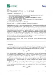
developed the inertial RFW process which uses a pre-loaded inertia wheel to have the power required by the welding. In 1960, RFW was used in the US to weld the oil drilling rods and the rst industrial machine was made in 1961. In the 70s, the direct driven RFW was used in aeronautical industry and in the 90s, the inertial RFW process was used for the largest parts. The RFW process allows to weld two dierent parts of which one at least has a cylindrical shape. The direct driven process may be divided into four stages:

Figure 1.1:

The four stages of the RFW process

Stage 1: The two parts are put in the machine: the cylindrical one in a spindle and the other one in a stationary vice. The spindle is attached to the motor and is put to a prescribed rotary speed. Stage 2: Initial contact. A pre-determined pressure is applied at the bottom of the rotating part and puts the two parts in contact. The contact is maintained until the friction removes the surface irregularities. The frictional heating starts. Stage 3: The mechanical energy is converted into heat energy and mechanical deformation to increase the temperature at the welding interface. This temperature is generally very close to the melting temperature and a plasticized layer is created at the interface. The incompressibility of this layer leads to the formation of ashes, which leads to the component shortening, also called upset. Stage 4: Forge. The motor is stopped. A larger force is applied in order to end the welding


Direct Driven Rotary Friction Welding Process (RFW)

5

by removing the last remaining impurities via the ashes. The temperature is decreasing. After a certain time, the components are unloaded and removed from the machine for the nal cooling-down.

Figure 1.2:

Weldable materials [www.ardindustries.com]

Compared to other welding processes, such as TIG (Tungsten Inert Gas), EBW (Electron Beam Welding), plasma and laser, RFW has many advantages. First of all, there is no porosity default at the interface since they are all ejected in the ashes. Then, there is no material addition and the welding is of forged type. Hence the characteristics of the welding are in general at least as good as the one of the welded materials separately. The microstructure of the welding area is of wrought type, which means that unweldable material can be welded such as Nickel superalloy. It is also possible to weld together dierent materials as shown on gure 1.2.


6

Introduction

1.3 Current RFW modeling using Finite Elements Method (FEM) The mechanical computation of the RFW process using a Finite Element (FEM) approach is now relatively well known. At the beginning, studies used to consider only a purely thermal model. In 1990, Sluzalec [Sªu»alec, 1990] modeled the driven RFW considering the thermo-mechanical coupling. During the last twenty years, numerous researches have also been conducted considering the coupling for the inertia RFW process [Soucail et al., 1992] [Moal and Massoni, 1995]. Commercial codes, like Abaqus for instance [Simulia Abaqus, 2010], propose the necessary scripts to "easily" run the coupled thermo-mechanical computation using FEM.

Figure 1.3:

Remeshing steps during Abaqus computation of RFW [Simulia Abaqus, 2010]

The results obtained with FEM are close enough to experimental data to be considered as a reliable prediction, even when the welding of two dissimilar materials is modeled [D'Alvise et al., 2002]. However, standard FEM may not be the most adapted method to model this process since they also present some drawbacks. Indeed, the thermo-mechanical coupling has a very important role and requires a high accuracy level, which the FEM might not reach because of the large deformations. To handle the large deformations, FEM computations proceed to a certain number of remeshing steps as shown on gure 1.3. Studies put in evidence that in general, adaptive meshes may give reasonable prediction but may also totally miss certain physi-


Objectives of this work

7

cal phenomena such as wrinkling and shear band phenomena [Lee and Bathe, 1994]. Moreover, the accuracy on the thermal eld might not be sucient for metallurgy purpose.

2 Objectives of this work Control of the direct driven RFW process is achieved by manipulating three main operating parameters: the rotary speed ω(t), the torque N (t) and nally the pressure P (t) applied on the bottom of the rotary part. The use of experimental trials to determine optimum process parameters has proven eective but a substantial number of test pieces are required to nd the good settings. The empirical approach is expensive and lacks exibility in term of geometry and design optimization. Finite Element computations are eective but require a substantial number of remeshing steps, which represent a loss of time but also a loss of accuracy because of the transfer of the dierent elds from the old mesh to the new one. On the other hand, meshless methods have some superiors features compared to conventional grid-based methods such as FEM. The most relevant argument in this context is that meshless methods can easily handle large deformation because of the absence of any mesh: they need no mesh generation, suer no mesh distortion nor mesh alignment sensitivity and no remeshing are necessary. The other main advantages are the high smoothness of the shape functions, the generally better convergence and nally that the volumetric locking may be alleviated by tuning the dilation parameter of the kernel function. The aim of this study is to develop and propose a meshfree approach based on the Local Maximum Entropy method (LME). This approach must be able to predict the temperature, heat aected zone dimensions, material shortening (upset), stress, residual stress and strain elds. This code should bring to the industry a representation correct enough to be able to perform microstructure studies. LME basis functions have been used in computational mechanics for only a few years but already provide very impressive results, especially in the modeling of high velocity impacts in the Optimal Transportation Method (OTM) of Li et al. [Li et al., 2010]. Therefore, it is expected that a LME approach should give good results in the modeling of the RFW.

3 Meshless approximations A multitude of dierent meshless methods has been published in the last decades. Despite the number of methods, there are signicant similarities between many of them and the major dierence lies in the manner of constructing the approximation of a single function u(x) in the domain based on a set of scattered nodes. This section will describe the most common approximations used for meshless methods.


8

Introduction

Cueto and Chinesta [Cueto and Chinesta, 2013] recently made a review about the eciency of dierent meshless methods for the simulation of material forming.

3.1 Smooth Particle Hydrodynamics (SPH) Smooth Particle Hydrodynamics (SPH) has been introduced in 1977 by Lucy [Lucy, 1977] and Gingold and Monaghan [Gingold and Monaghan, 1977] and is one of the earliest particle method. SPH basically consists in approximating a function u(x) on a domain Ω by a convolution. Z x−y h u (x) = Cp Φ( )u(y)dy (1.1) ρ Ω where uh is the approximation of u, Φ is a function dened on a compact usually called weight, window function or kernel function and ρ is the dilation parameter. Cp is called normality property of the window function and is a constant such that Z y (1.2) Cp Φ( )dy = 1 ρ Ω The discrete SPH form is obtained using numerical quadratures

uh (x) =

X

Cp Φ(

a

x − xa )ua ωa ρ

(1.3)

where xa are the nodes called particles and ωa are the weights of the associated quadrature. ua ≡ u(xa ) is the value of the original function u at particle xa . The discrete window function is dened by

w(x − xa , ρ) = Cp Φ(

x − xa ) ρ

(1.4)

Therefore, the SPH meshless approximation can be dened by

uh (x) =

X

Na (x)ua

(1.5)

a

with the approximation basis Na (x) = w(x − xa , ρ)ωa . The window function Φ plays an important role in this meshless method. It is required to satisfy the following conditions [Monaghan, 1982]: w(x − xa , ρ) > 0 on a subdomain Ωa of Ω; w(x − xa , ρ) = 0 outside of the subdomain Ωa ; w(x − xa , ρ) → δ(x − xa ) the Dirac function as ρ → 0; w( . , ρ) is a monotonically decreasing function.


Meshless approximations

9

The three most commonly used window functions are the cubic spline, Gaussian and quartic spline. For example, let da = ||x − xa ||, r = da /dmax with dmax the size of a a the support of the a-th particle. The window functions can be written as a function of the normalized radius r:

cubic spline : w(r) =

 

2 3 4 3

− 4r2 + 4r3 − 4r + 4r2 − 34 r3

 0 (

exp(−(αr)2 )−exp(−α2 ) 1−exp(−α2 )

Gaussian: w(r) = quartic spline: w(r) =

0

1 − 6r2 + 8r3 − 3r4 0

for r ≤ 12 for 21 < r ≤ 1 for r > 1 for r ≤ 1 for r > 1 for r ≤ 1 for r > 1

(1.6a) (1.6b) (1.6c)

Even if the continuous form of SPH meshless approximation is zeroth-order complete and most of the window functions satisfy higher order consistency condition, the discrete SPH form is not able of even reproducing constant elds and hence, is not a partition of unity. The conditions for zeroth-order and rst order consistency are:

X

Na (x) = 1

(1.7a)

Na (x)xa = x

(1.7b)

a

X a

Consistency is generally necessary for convergence, which directly contributes to the interpolation error. Corrections must be made to the window functions for convergence and accuracy of SPH method. Numerous improvements have been developed to fulll the completeness: Johnson-Beissel correction [Johnson and Beissel, 1996], Randles-Libersky correction [Randles and Libersky, 1996], Krongauz-Belytschko correction [Belytschko et al., 1998], Monaghan's symmetrization on derivative approximation [Monaghan, 2005], etc. However, most of the analysis related to the convergence, stability and accuracy properties are based on uniformly distributed particles and the results obtained by such analysis are often limited to idealized circumstances. In general cases implying large deformations where the particles are disordered, the obtained results may not always be reliable since the eect of the particle irregularity on the accuracy of the solution is not very clear. Moreover, the SPH shape functions are not interpolant since uh (xa ) 6= ua and they do not verify the Kronecker delta property:

Na (xb ) 6= δab

(1.8)

Thus it is not easy to apply boundary conditions on nodes, which is absolutely necessary for the use of meshless method in solid mechanics, without special techniques.


10

Introduction

3.2 Moving Least Squares (MLS) The objective of the Moving Least Squares (MLS) is to obtain an approximation based on an array of nodes in the considered domain, but with high accuracy and high order of completeness. The MLS method was rst introduced in curve and surface tting by Lancaster and Salkauskas [Lancaster and Salkauskas, 1981] and then in solid mechanics in the diuse element method by Nayroles et al. [Nayroles et al., 1992]. Other studies and applications are made in the ElementFree Galerkin (EFG) methods by Belytschko et al. [Belytschko et al., 1994]. Basically MLS is about approximating u(x) through a polynomial of order m with non-constant coecients in the domain: h

u (x) =

m X

(1.9)

pi (x)bi (x) = pT (x)b(x)

i

where p0 (x) = 1 and pi (x) are monomials in the space coordinates x = (x1 , ..., xd )T ∈ Rd so that the basis is complete. For example, in one dimension, a complete polynomial p of order m is

p(x) = (1, x, x2 , ..., xm )T

(1.10)

b(x) = (b0 (x), b1 (x), b2 (x), ..., bm (x))T

(1.11)

and b(x) is given by

where the unknown parameters bi (x) at any given point are determined by minimizing the dierence of a weighted discrete L2 -norm between the local approximation at that point and the nodal parameter ua as follow: inf J with J = b

n X

w(x − xa )(uh (xa ) − ua )2 (1.12)

a=1

=

n X

T

2

w(x − xa )(p (xa )b(x) − ua )

a=1

where w(x − xa ) is a window function with compact support as mentioned in SPH methods, n is the number of nodes in the neighborhood of x and ua is the nodal value of u at x = xa . The stationarity of J in equation 1.12 with respect to b(x) leads to a linear relationship between b(x) and ua :

b(x) = A−1 (x)B(x)u


(1.13)


11

where

A(x) =

n X

wa (x)p(x) ⊗ p(x)

(1.14a)

a=1

B(x) = [w1 (x)p(x1 ), w2 (x)p(x2 ), ..., wn (x)p(xn )]T

(1.14b)

u = [u1 , u2 , ..., un ]T

(1.14c)

Hence, the approximation uh (x) is h

u (x) =

n X

Na (x)ua

(1.15)

a=1

where the shape function related to node a is

Na (x) =

m X

pi (x)(A−1 (x)B(x))ia

(1.16)

i=0

The MLS approximation perfectly reproduces all the polynomials in p(x). Therefore, the consistency of order m is satised by the MLS approximation if the basis is complete in the polynomials of order m. However, the main drawback of the MLS is the eciency: in order to obtain an accurate shape function and compute the inverse matrix A−1 , the number of nodes in the inuence domain is usually much greater than the number of monomials in the polynomial basis, especially in two or three dimensions. It also must be noted that MLS does not satisfy the Kronecker delta criterion either, therefore associated shape functions are not interpolant: the nodal parameters ua are not the nodal values of uh (xa ) and the approximation on the boundary of the domain may depend on the nodal data of interior nodes. Just like SPH, this property makes the imposition of boundary conditions more complicated than with nite elements.

3.3 Reproducing Kernel Particle Method (RKPM) The Reproducing Kernel Particle Method (RKPM) introduced by Liu et al. [Liu et al., 1995] is an improvement of the continuous SPH approximation. A correction function C(x, y) is introduced into equation 1.1 in order to increase the order of completeness of the approximation Z x−y h )u(y)dy (1.17) u (x) = C(x, y)Φ( ρ Ω where K(x, y) = C(x, y)w(x − y, ρ) is dened such that the approximation is m-th order consistent. Suppose that p(x) is a complete array of monomial up to m-th order. Then any m-th order polynomials can be written

u(x) = pT (x)b


(1.18)

12

Introduction

where b are the unknown coecients. Then Z Z T p(y)w(x − y, ρ)u(y)dy = p(y)p (y)w(x − y, ρ)dy b Ω

(1.19)

Ω

which is a system of equations for b. A substitution in equation 1.18 leads to

h

T

Z

−1 Z

T

p(y)p (y)w(x − y, ρ)dy

u (x) = p (x) Ω

p(y)w(x − y, ρ)u(y)dy (1.20)

Ω

Thus the correction function is

T

Z

−1

T

p(y)p (y)w(x − y, ρ)dy

C(x, y) = p (x)

= pT (x) (M (x))−1 p(y)

Ω

The discrete RKPM form is obtained using numerical quadratures

uh (x) =

n X

(1.21)

C(x, xa )w(x − xa )ua ωa

a=1 −1

T

= p (x)(M (x))

n X

(1.22)

p(xa )w(x − xa )ua ωa

a=1

Numerical integration is also required to evaluate the moment matrix M (x) Z M (x) = w(x − y, ρ)p(y)pT (y)dy Ω

=

n X

w(x − xa , ρ)p(xa )pT (xa )ωa

(1.23)

a=1

Just like the SPH approximation, RKPM does not verify the Kronecker delta property and special techniques are needed to impose essential boundary conditions such as described by Chen [Chen et al., 1997].

3.4 Natural Element Method (NEM) The Natural Element Method (NEM) introduced by Sukumar [Sukumar, 1998] [Sukumar and Moran, 1999] [Sukumar et al., 2001] is the rst really successful attempt for a method free of error in the interpolation of the essential variable along the boundary. The NEM was originally a Galerkin method in which the interpolation was achieved through natural neighbor (NN) methods [Sibson, 1980] [Sibson, 1981] [Belikov et al., 1997] [Belikov and Semenov, 2000]. More recently, a book has been written by Chinesta et al. [Chinesta et al., 2013] about the use of the NEM in the simulation of structures and processes.



13

As Element Free Galerkin Method (EFGM) [Belytschko et al., 1994], NEM constructs the connectivity of each material point using the concept of Delaunay triangulation. The advantage of the NEM is the good accuracy provided despite the distortion of this triangulation, as proved by Sukumar [Sukumar, 1998]. The Delaunay triangulation [Delaunay, 1934] of a cloud of nodes X = {x1 , x2 , ..., xn } ⊂ Rd is the unique triangulation of the cloud that satisfy the so-called circumcircle criterion. The dual structure of the Delaunay triangulation is the Voronoi diagram. It is composed by a tessellation of the space into cells of the form

Txa = {x ∈ Rn | ∀b 6= a, d(x, xa ) < d(x, xb )}

(1.24)

where Ta represents the Voronoi cell and d(., .) the Euclidean distance. The most popular natural neighbor (NN) interpolant is due to Sibson [Sibson, 1981]. Consider the second-order Voronoi cell:

Txa ,xb = {x ∈ Rn | ∀c ∈ / {a, b}, d(x, xa ) < d(x, xb ) < d(x, xc )}

(1.25)

Then the Sibsonian shape function is dened as

φa (x) =

Aa (x) A(x)

(1.26)

P where Aa (x) is the Lebesgue measure of the cell Tx,xa and A(x) = na=1 Aa (x) is the Lebesgue measure of the cell Tx . The NN interpolation dened by these shape functions has remarkable properties. First, the partition of unity property is veried: n X

φa (x) = 1

(1.27)

a=1

The partition of unity property implies the non-negativity and convexity of trial function: 0 ≤ φa (x) ≤ 1 (1.28) Moreover, the cardinal, or Delta-Kronecker, property is fullled and the shape functions are interpolant: φa (xb ) = δab , uh (xa ) = ua (1.29) The linear completeness property (it can exactly reproduces linear displacement elds) is also veried: n X x= φa (x)xa (1.30) a=1

The supports of the shape functions are compact, and hence a local interpolation scheme is realized. Finally, the shape functions are smooth (C 1 ) everywhere except at the nodes where they are simply continuous (C 0 ).


14

Introduction

Despite the interesting properties of NN interpolation, the main drawback of NEM is its high computational cost, especially for Sibson interpolation. An analysis of the computational cost of several meshless method was made by Alfaro et al. [Alfaro et al., 2006]. It is shown that mesh distortion could lead to important inaccuracies when using FEM while Sibson interpolation is several orders of magnitude heavier to compute than traditional piecewise polynomial shape functions for nite elements. However, in non-linear computations, while frequent Newton-Raphson iterations are needed, the relative cost of shape function is obscured by the cost of updating tangent stiness matrix.

3.5 Material Points Method (MPM) The Material Point Method (MPM) introduced by Sulsky et al. [Sulsky et al., 1993] [Sulsky et al., 1995] is an extension of the particle-in-cell method [Evans et al., 1957]. This method is not about interpolating but about being able to consider the history dependency of the constitutive equations in a broad class of engineering problems such as penetration, impact or large rotations of solid bodies. It is a discrete solution procedure for computational solid mechanics which is generalized using a variational form and a Petrov-Galerkin discretization scheme, resulting in a family of methods named the Generalized Interpolation Material Point (GIMP) [Bardenhagen and Kober, 2004]. The essential idea is to take advantage of both the Eulerian and Lagrangian methods, which can be summarized as follows. If a continuous material under a purely mechanical loading is considered, the governing dierential equations can be derived from the conservation equation of mass

dρ + ρ∇ · v = 0 dt

(1.31)

and the conservation equation of momentum

ρa = ∇ · s + ρb

(1.32)

supplemented with a suitable constitutive equation and kinematic relations between strain and displacement. In the equations 1.31 and 1.32, ρ(x, t) refers to the mass density, v(x, t) is the velocity, a(x, t) is the acceleration, s(x, t) is the Cauchy stress tensor, b(x, t) is the specic body force and x is the current position at time t of any material point. The key dierence among dierent spatial discretization methods is the way in which the gradient and divergence terms are calculated. The MPM discretizes a continuous body by using a nite set of np material points in the original conguration that are tracked throughout the deformation process. Let xti , i ∈ {1, .., np } denote the current position of material point p at time t. Each material point at time t has an associated mass Mp , density ρtp , velocity vpt , Cauchy



15

stress tensor stp , strain etp and any other internal state variables necessary for the constitutive model. Thus these material points provide a Lagrangian description of the continuous body. Since each material point contains a xed amount of mass for all time, equation 1.31 is automatically satised. At each time step, the information from the material points is mapped to a background computational mesh (grid). This mesh covers the computational domain of interest and is chosen for computational convenience. After the information is mapped from the material points to the mesh nodes, the discrete formulation of equation 1.32 can be obtained on the nodes. By using the same procedure used in FEM, the weak form of equation 1.32 is given by Z Z Z Z s s ρw · a dΩ = − ρs : ∇w dΩ + ρc · w dS + ρw · b dΩ (1.33) Ω

Sc

Ω

Ω

where w is the test function, ss = ρ1 s is the specic stress, Ω is the current conguration of the material, S c is the part of the boundary subject to a traction and w is assumed to be zero on the boundary with a prescribed displacement. Since the whole continuum body is described with the use of a nite set of material points, the mass density at a general position x is

ρ(x, t) =

np X

Mp δ x − xtp

(1.34)

p=1

where δ is the Dirac delta function (with dimension of the inverse of a volume). In other words, the mass is non-null only at the material points. The substitution into equation 1.33 converts the integrals into the sums of quantities evaluated at the material points: np X

Mp w xtp , t · a xtp , t

p=1

=

np X

h i Mp −ss xtp , t : ∇w|xtp + w xtp , t · cs xtp , t h−1 + w xtp , t · b xtp , t

p=1

(1.35) with h the thickness of the boundary layer. The interactions among dierent material points are reected only through the gradient terms, and a suitable set of material points must be chosen to represent the boundary layer. In the MPM, a background computational mesh is required to calculate the gradient terms. To do so, we suppose that a computational mesh is constructed, using 2-node cells in 1D,


16

Introduction

3-node cells in 2D and 4-node cells in 3D for example. These cells are then employed to dene standard FEM nodal basis functions Ni (x) related to the spatial nodes xi (t) with i ∈ {1, ..., n} where n is the total number of mesh nodes. The coordinates of any material point in a cell can be represented by

xtp

=

n X

xti Ni xtp

(1.36)

i=1

In the same way, the displacement of any material point in a cell are dened by the nodal displacement uti (t). Therefore:

utp

=

n X

uti Ni xtp

(1.37)

i=1

Since the same basis functions are used for both spatial coordinates and displacements, kinematic compatibility demands that the basis functions advect with the material, as in the updated Lagrangian framework. In other words, the material time rates of the basis functions must be zero. Hence, it follows that the velocity and acceleration of any material point in a cell are represented by

vpt =

n X

vit Ni xtp

(1.38)

i=1

and

atp

=

n X

ati Ni xtp

(1.39)

i=1

where vpt and atp are respectively the nodal velocities and accelerations. The test function is also dened by n X t wp = wit Ni xtp (1.40) i=1

Those equations ensures that the associated vectors are continuous across the cell boundary. However, their gradients are not continuous due to the the use of linear shape functions. Substituting equations 1.39 and 1.40 into equation 1.35 yields np X

wit

·

np X

p=1

mtij atj

p=1 np

=−

X p=1

wit

·

np X p=1

Mp s

s,t

· ∇Ni |xtp +

n X i=1

wit

·

cti

+

n X

wit · bti

i=1

at time t. In equation 1.41, the consistent mass matrix is given by


(1.41)


17

mtij

=

np X

(1.42)

Mp Ni xtp Nj xtp

p=1

with corresponding lumped nodal masses

mti

np X

=

Mp Ni xtp

(1.43)

i=1

The discrete specic traction is then

cti

=

np X

−1 t Mp cs,t p h Ni xp

(1.44)

p=1 s with cs,t p = cp

xtp , t while the specic body force is discretized as bti

=

np X

Mp bta Ni xtp

(1.45)

p=1

s t with bs,t = b x , t . One should notice that if b is a known function of position and p p p time, as gravity for instance, then the nodal body force can be computed directly by bti = b xtp , t mti . Since the wit are arbitrarily chosen except where the components of displacement are prescribed, for a lumped mass matrix, equation 1.41 simply becomes: mti ati = fit

int

+ fit

ext

(1.46)

where the internal force is given by:

int fit

=−

np X

t Mp ss,t p · Gi x p

(1.47)

p=

t t s with ss,t p = s xp , t , Gi xp ) ∇Ni |xtp and the external force is fit

ext

= cti + bti

(1.48)

As shown in the previous equations, the information is mapped from material points to the nodes of the cell containing these points through the use of shape functions. The key feature of MPM is the use of the same set of nodal basis functions for both the mapping from material points to cell nodes to solve equation 1.46 and the mapping from cell nodes to material points to update the material point information for the next time step. This method has the advantage to be able to handle large deformation but just like the methods presented previously, it is very dicult to apply boundary conditions [Chen and Brannon, 2002]. Finally, MPM can only be used for isothermal mechanics analysis.


18

Introduction

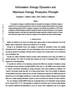
3.6 Optimal Transportation Meshfree (OTM) method: an example of LME interpolation use The Optimal Transportation Meshfree (OTM) method has been developped by Li et al. [Li et al., 2010] a few years ago to simulate general solid and uid ows, including uid-structure interaction, and is mostly used to perform high velocity impact simulations such as the ones presented on gure 1.4. It combines the MPM approach and the maximum entropy interpolation (see chapter 2) in order to generalize the Benamou-Brenier dierential formulation of optimal mass transportation problems to problems including arbitrary geometries and constitutive behaviors.

Figure 1.4:

Three high velocity impact simulations using OTM on a metallic target with distinct thicknesses.

The algorithm used to run a mechanical simulation is the following:

Algorithm OTM - Elastic solid ow [Li et al., 2010] 1. Initilization: Set k = 0, initialize nodal coordinates xa,−1 , xa,0 , shape functions Na,0 , material points coordinates xp,0 , volumes vp,0 , densities ρp,0 and deformation gradients Fp,0 . 2. Compute mass matrix Mk , linear moment lk and internal forces fk (same as MPM). 3. Update nodal coordinates:

xk+1 = xk + (tk+1 −

tk )Mk−1

tk+1 − tk−1 lk + fk 2

4. Update material point coordinates using the LME basis functions φ:

xp,k+1 = φh,k→k+1 (xp,k )


Thesis outline

19

5. Update material point volumes:

vp,k+1 = det ∇φh,k→k+1 (xp,k )vp,k 6. Update material point mass densities:

ρp,k+1 =

mp vp,k+1

7. Update material point deformation gradients and right Cauchy-Green deformation tensors: Fp,k+1 = ∇φh,k→k+1 (xp,k )Fp,k T Cp,k+1 = Fp,k+1 Fp,k+1

8. Recompute shape functions Na,k+1 (xp,k+1 ) and derivates ∇Na,k+1 (xp,k+1 ) from updates nodal set. 9. Reset k ← k + 1. If k = N exit. Otherwise go to (2). Our work and the OTM method have a lot in common: the use of material points and the LME basis functions (see chapter 2). The main dierence is that the OTM method has a dynamic approach based on the optimal transportation principle whereas out work is based on a Galerkin approach (the mass matrix is assumed to be constant). The current limitations of the OTM method are that it is somewhat restricted to use an explicit time integration scheme and cannot simulate conduction problems and thus cannot perform coupled thermo-mechanical analyses.

4 Thesis outline In this thesis, we aim at building a meshless method using the Local Maximum Entropy (LME) interpolation combined to a strongly coupled thermo-mechanical variational formulation. The objective is to be able to model coupled thermomechanical problems with large deformation which may include complex boundary conditions such as contact and/or convection. In chapter 2, we present an energy-based variational modeling of strongly coupled thermo-mechanical problems adapted to a meshless method. We rst present the time-continuous evolution problem and its variational formulation, followed by the time-discrete (or incremental) variational formulation and nally the timed-space-discrete variational formulation considering the meshless environment. Then some ow stress models are presented considering the variational framework. In chapter 3, the LME interpolation approach is described. The construction of LME shape functions and how the LME-based meshless method is working are


20

Introduction

detailed. A particular attention is paid to the localization of the material points. Then, some features are exposed and nally, we present some adjustments needed to work in an updated-Lagrangian framework. In chapter 4, test cases are proposed in order to verify our implementation of the LME-based meshless method. From a simple conduction test to a tensile test considering conduction, convection, large deformation and coupled thermo-viscoplasticity passing by some classical benchmark tests as the Taylor bar or the patch test, the possibilities, but also the limits, of our implementation are exposed. Finally, the chapter 5 is dedicated to the modeling of the RFW process. We are presenting some specic modules implemented such as the contact in the friction area and the resulting heat ux. Numerical results are then presented and analyzed, in the light of available experimental observations.


Chapter 2 Thermo-mechanical problem

A variational approach is proposed for the modeling of strongly coupled thermo-mechanical problems. In this chapter, variational formulations and associated principles are described and used to establish the variational thermo-mechanical framework that is used in our implementation. Then, some ow stress models are presented and the associated stored and dissipative plastic energy are detailed.


Contents 1

Energy-based variational method and variational principles 23

1.1 1.2 1.3 1.4 1.5

2

23 24 24 25 26

Variational formulation in thermo-mechanical coupling . . . . Discretized variational formulation . . . . . . . . . . . . . . .

28 31

Variational framework and ow stress models . . . . . . . . 36 3.1 3.2 3.3 3.4

4

. . . . .

General framework . . . . . . . . . . . . . . . . . . . . . . . . 28 2.1 2.2

3

Hamilton's principle . . . . . . . . . . . . . . . . . . . . . . Hu-Washizu-Fraeijs de Veubeke's principle . . . . . . . . . . Hellinger-Reissner's principle . . . . . . . . . . . . . . . . . Minimum potential energy principle . . . . . . . . . . . . . Balance equations in local coupled thermo-dynamical model

Power law ow stress model . . . . Norton-Ho ow stress model . . . Johnson-Cook ow stress model . . Zerilli-Armstrong ow stress model

. . . .

. . . .

. . . .

. . . .

. . . .

. . . .

. . . .

. . . .

. . . .

. . . .

. . . .

. . . .

. . . .

. . . .

. . . .

37 38 39 41

Conclusion . . . . . . . . . . . . . . . . . . . . . . . . . . . . . . 41


Energy-based variational method and variational principles

23

1 Energy-based variational method and variational principles Variational principles have played an important role in mechanics for several decades [Lanczos, 1970] and have been mostly developed for conservative systems. The most eminent examples are Hamilton's principle [Hamilton, 1834] in dynamics and the principle of minimum potential energy in statics. Some variational principles are also used for dissipative systems, such as principles of maximum plastic dissipation for limit analysis. From a mathematical but also numerical point of view, variational approaches present many attractive features such as unicity, convergence and stability of the formulations. This has motivated a lot of interest following the pioneering work of Biot [Biot, 1956]. It as well concerns isothermal settings such as elasto-viscoplasticity [Comi et al., 1991] [Ortiz and Stainier, 1999] or isothermal brittle and ductile damage [Francfort and Marigo, 1998] [Balzani and Ortiz, 2012] and coupled thermo-elastic and thermo-visco-elastic problems [Herrmann, 1960] [Batra, 1989]. Basically, a variational principle is an optimization approach used to derive the balance and the evolution equations of a boundary values problem. The most popular principles are Hamilton's and Veubeke-Hu-Washizu's. Let us dene φ(t) as the transformation mapping describing the state of the system at the time t [Marsden and Hughes, 1994]. We then seek to write variational principles determining the evolution of the system, in a dynamical or quasi-constant setting.

1.1 Hamilton's principle Hamilton's principle [Hamilton, 1834] is a statement that the dynamics of the physical system can be determined by an unique function, the Lagrangian, which contains all physical information concerning the system and the forces acting on it. Hamilton's principle states that the true evolution φ(t) of a system between two specied times t1 and t2 is a stationary point for the functional

Z

t2

S(φ) =

˙ L φ, φ, t dt

(2.1)

t1

˙ t is the Lagrangian. In other word, the evolution φ(t) of a system where L φ, φ, is the solution of ∀δφ, Dφ [S (φ)] (δφ) = 0


(2.2)

24

Thermo-mechanical problem

1.2 Hu-Washizu-Fraeijs de Veubeke's principle Hu-Washizu-Fraeijs de Veubeke's principle [Washizu, 1955] [de Veubeke, 1972] [Hu, 1984] is the canonical principle of static elasticity. It depends on three independant elds which are: the conguration φ, the deformation gradient F and the Piola stress tensor P . The associated functional H (φ, F , P ) is dened by

Z H (φ, F , P ) =

W (F T F ) + P · (∇φ − F ) dV −

B0

Z

Z ρ0 b · φ dV −

B0

t · φ dA ∂σ B0

(2.3) where W is the inner elastic strain energy depending on the Cauchy-Green tensor C = F T F to ensure the independence of the coordinate system, b is the body forces (gravity for instance) and t the imposed force applied on the part ∂σ B0 = ∂B0 \∂φ B0 of the external surface of the body. Then, the quasi-static evolution of the system is described by a sequence of equilibrium status, each satisfying the variational principle inf

φ,F

adm.

sup H (φ, F , P )

(2.4)

P

An admissible conguration φ must verify the essential boundary conditions φ = φ on ∂φ B0 . An admissible deformation gradient F must verify the material impenetrability condition det F > 0. Every tensor can be an admissible stress tensor P. The Gâteaux derivatives Dφ [H (φ, F , P )] (δφ), DF [H (φ, F , P )] (δF ) and DP [H (φ, F , P )] (δP ) respectively yield the static equilibrium equation 2.5, the constitutive equation 2.6 and nally the compatibility equation 2.7.

∇ · P T + ρ0 b = 0 ∂W (C) ∂C F = ∇0 .φ

P = 2F

(2.5) (2.6) (2.7)

Thus, the stress Piola-Kirchho tensor is given by

S = F −1 P = 2

∂W (C) ∂C

(2.8)

1.3 Hellinger-Reissner's principle Hellinger-Reissner's principle is obtained from the previous principle. Let us introduce the complementary strain energy density, obtained by a Legendre transformation of the energy density 1 ∗ W (S) = sup S : C − W (C) (2.9) 2 C LME interpolation approach for coupled thermo-mechanical problems


25

The inverse transformation is

W (C) = sup S

1 ∗ S : C − W (S) 2

(2.10)

If the compatibility equation F = ∇φ is veried, then we obtain the functional

Z Z 1 T ∗ S : (∇φ ∇φ) − W (S) dV − ρ0 bφ dV − H (φ, S) = tφ dA B0 2 B0 ∂σ B0 (2.11) and the boundary value problem has the following variational form: Z

φ

inf

adm.

sup H (φ, S) S

(2.12)

adm.

1.4 Minimum potential energy principle As an example, let us consider how the minimum potential energy principle is used to build the variational modeling. If the compatibility equation 2.5 and the constitutive equation 2.6 are assumed veried, then the functional 2.3 becomes [Marsden and Hughes, 1994]

Z H (φ) =

Z

Z

T

ρ0 bφ dV −

W (∇0 φ ∇0 φ) dV − B0

tφ dA

(2.13)

∂σ B0

B0

= U(φ) − W(φ) with the potential strain energy

Z U(φ) =

W (∇0 φT − ∇0 φ) dV

(2.14)

B0

and the energy from external forces Z Z W(φ) = ρ0 bφ dV + B0

tφ dA

(2.15)

∂σ B0

where ρ0 is the mass density, b is the body force, ∇0 is the material gradient and t the imposed force. Assuming the compatibility condition and constitutive relations are satised, the boundary value problem via variational principle is described by φ

inf (U(φ) − W(φ)) adm.

(2.16)

Its stationary point with respect to φ corresponds to the conservation of momentum in elasticity (see equation 2.19).


26


As illustrated by many examples, the variational form of equations is very convenient for the numerical simulations, and the uniqueness and existence of the solutions in the problem are easily analyzed from a mathematical point of view. By means of this energy-based variational method, we emphasize that a physical problem is transformed to a mathematical optimization, and then a series of optimization algorithms can be applied in the analysis of physical elds.

1.5 Balance equations in local coupled thermo-dynamical model The variational formulation of a coupled thermo-mechanical problem includes the three classical conservation equations of mechanics:

• Conservation of mass ρ det F = ρ0

(2.17)

where ρ is the mass density in the deformed conguration, ρ0 is the mass density in the initial conguration and F is the deformation gradient.

• Conservation of linear momentum ¨ = ∇0 · P T + ρb ρ0 φ

(2.18)

where P is the rst Piola-Kirchho (or Piola) stress tensor and b represents the applied bulk forces per mass unit.

• Conservation of angular momentum PFT = FPT

(2.19)

The thermo-mechanical coupling involves two more conservation laws which represent the laws of thermo-dynamics:

• Conservation of energy (rst law of thermo-dynamics) ρ0 T η˙ = P : F˙ + Y d : Z˙ − ∇0 · H + ρ0 Q

(2.20)

where H is the nominal (Lagrangian) heat ux vector, Q the applied bulk heat source (per mass unit) and η is the internal entropy density (per mass unit).

• Clausius-Duhem Inequality (second law of thermo-dynamics) 1 (2.21) T Γ˙ = Dint − H · ∇T ≥ 0 T where T is the absolute temperature and Γ˙ denotes the net entropy production rate.



27

Furthermore, a boundary value problem is described by the above governing equations including material constitutive relations and compatibility conditions. According to the variational method, by multiplying a small constrained but arbitrary variation l ∈ V = {l ∈ R3 |l = 0 on the boundaries}, the weak form of the problem can be obtained. For instance, consider the following mechanical problem:

∇0 · P T + ρ 0 B = 0 P · n = τ on L

(2.22)

where τ is the traction on the boundary L. The weak form is dened by Find φ ∈ P such that ∀l ∈ V, G(φ, l) = 0 where

Z

Z (P : ∇l − ρ0 B · l) dV −

G(φ, l) = V

τ · l dL

(2.23) (2.24)

L

with φ ∈ P = φ ∈ R3 |φ = φ in the boundaries . If the physical elds and l are C 1 , the weak form is equivalent to the strong form. In view of the weak form, Marsden and Hughes [Marsden and Hughes, 1994] pointed out that there is a potential E such that Dφ E(φ) · l = G(φ, l) if, and only if, ∀φ ∈ P, ∀(l, ξ) ∈ V 2 , D1 G(φ, l) · ξ = D1 G(φ, ξ) · l

(2.25)

and its corresponding form is

Z E(φ) =

1

G(tφ, φ) dt

(2.26)

0

Thereby, a formulation embodying equilibrium equations, material behaviors and boundary condition is built in the variational framework. Even if the weak form of conservation laws seems to be a basis to build the variational pseudo-potential, the symmetry still has to be guaranteed. In 1999, Ortiz and Stainier [Ortiz and Stainier, 1999] obtained a variational formulation for general viscoplastic solids with respect to dierent dissipative relations in nite deformation regime. They developed a constitutive update modeling as an optimization to a scalar function with a set of internal variables, including Hemholtz free energy, conjugate inelastic potential and viscous part. The associated constitutive updates can be dened by minimization of an incremental pseudopotential about deformation over the time step. This work represents a new and active research area, the applications of this variational structure to general dissipative materials are continuously developed [Stainier et al., 2002]. For instance, constitutive visco-elastic formulations are as following provided to embody the nonlinear viscous behavior based on this theoretical framework [Stainier et al., 2005] [Fancello et al., 2006] [Mosler and Bruhns, 2009] [Weinberg et al., 2006].


28


By considering temperature eects, a variational formulation of thermo-mechanical boundary-value problems was proposed by Yang et al. [Yang et al., 2006]. They introduced the equilibrium temperature in the formula, thus making the weak form symmetric. In addition, the characteristic of this formulation is that it allows to describe the thermal and mechanical balance equations, including irreversible and dissipative behaviors, as an optimization of an energy-like variational form. In addition, beyond unifying a wide range of constitutive models in a common framework, the variational formulation also presents the interesting mathematical properties, like symmetry of its bilinear form, which is an important feature compared to the alternative coupled thermo-mechanical formulations. By applying this variational formulation, Stainier [Stainier and Ortiz, 2010] successfully presented an experimental validation of three thermo-viscoplastic materials: aluminum alloy, α-Titanium and Tantalum. These theoretical conclusions will be used to build a meshless solver for nite thermo-mechanical problems such as RFW modeling.

2 General framework 2.1 Variational formulation in thermo-mechanical coupling Thermo-mechanical couplings are a common phenomenon in solid mechanics, and associated eects are of importance in the manufacturing of parts and structures. For general dissipative materials, the thermo-mechanical coupling can easily provoke some localization zones associated with large deformation and high temperature, e.g. the formation of adiabatic shear bands [Su et al., 2014]. Their occurrence is a precursor to material macroscopic fracture. Here we are considering a strongly coupled boundary value problem. Thus the ve conservation laws detailed previously should be respected. The corresponding nite constitutive equations for thermomechanical coupling can be given in local form as following [Yang et al., 2006]

∇0 · P T + ρ0 B = ρ0 V˙

(2.27)

FPT = PFT

(2.28)

E˙ = P : F˙ + ρ0 Q − ∇0 · H

(2.29)

H ρ0 Q +∇· ≥0 T T

(2.30)

γ˙ ≡ ρ0 η˙ −

where P is the rst Piola stress tensor, F is the deformation gradient, V˙ is the acceleration, ρ0 is the density (per mass unit) of the undeformed volume, B is the body force per mass unit, Q and H are the specied heat source (per mass unit) and the nominal heat ux. T is the absolute temperature. We assume the existence of H and of the free energy W (F , T ) such that η is the specic entropy dened by

ρ0 η = −

∂W ∂T


(2.31)

General framework

29

By using Legendre-Frenchel transform, the internal energy density E is dened:

E = sup (ρ0 ηT + W )

(2.32)

T

and has the property

∂E ∂(ρ0 η) Consider the general pseudo-potential dissipation ∆ dened by

(2.33)

˙ Z, T ) + φ∗ (F˙ , F , T )) − χ(H, T ) ∆ = Ψ∗ (Z,

(2.34)

T =

where Ψ , φ and χ are the kinetic potential, viscous potential (Kelvin-Voigt viscoelasticity) and conduction potential. Z represents the internal variables, such as cumulated plastic strain for thermo-visco-elastic material for instance. F is the deformation gradient. Let us dene P as the rst Piola-Kircho stress conjugate to F as ∗

∗

∂W (2.35) ∂F The alternate representations of constitutive relations can similarly be obtained by using the conjugate pairs of stress-strain tensors (Cauchy stress and Chauchy-Green strain, second Piola-Kirchho stress and Green-Lagrange nite strain, etc.). Let us dene Y the conjugate force to cumulated plastic deformation: P =

Y =−

∂W ∂Z

(2.36)

The evolution equations gives

∂Ψ∗ (2.37) ∂ Z˙ where Ψ∗ is a dual pseudo-potential obtained from a Legendre-Fenchel transform of kinetic potential Ψ dened by n o Ψ∗ = sup Y · Z˙ − Ψ (2.38) Y =

Y

and

∂Ψ Z˙ = ∂Y

(2.39)

Ψ∗ is convex, Ψ∗ (0) = 0, Ψ∗ ≥ 0

(2.40)

If

the second law of thermo-dynamics is veried. Therefore for thermo-visco-plasticity material, the rst law of thermo-dynamics can also be written

∂ 2W ∂ 2W ρ0 C T˙ = T : F˙ + T · Z˙ + Dint + ρ0 Q − ∇0 · H ∂T ∂F ∂T ∂Z LME interpolation approach for coupled thermo-mechanical problems

(2.41)

30


where Dint = Y · Z˙ is the intrinsic dissipation and C is the heat capacity dened as

ρ0 C = −T

∂ 2W ∂T 2

(2.42)

which depends on the temperature and state variables in the physical system. As shown in [Stainier and Ortiz, 2010] in nite plastic strains, the variational formulation naturally included provides an accurate formulation of the Taylor-Quinney parameter to calculate the ratio of intrinsic dissipation converted to total plastic power. The second law of thermo-dynamics can be simplied as

T Γ˙ = Dint −

1 H · ∇T ≥ 0 T2

(2.43)

where Γ˙ is the net entropy production rate. As the kinetic potential Ψ∗ is convex, if χ is convex then the Clausius-Duhem inequality is automatically veried. Based on the previously described thermo-dynamic framework, the energy-based variational formulation of the coupled thermo-mechanical boundary-value problem proposed by Yang [Yang et al., 2006] can be summarized. The potential for general standard dissipative materials is stated as following:

Z 1 T ˙ T ˙ ˙ ˙ ˙ dV F , Z, − ∇T Φ φ, T, η, ˙ Z = E − ρ0 T η˙ + ∆ Θ Θ T B Z Z ˙ − ρ0 B · φ dV − T · φ˙ dS B ∂T B Z Z T T dV − dS + ρ0 Q log H log T0 T0 ∂η B B

(2.44)

where T is the applied traction over the traction boundary ∂T B . H is the outward heat ux over the Neumann boundary condition ∂η B . In equation 2.44, the authors introduced two temperatures Θ and T , which are respectively an equilibrium or internal temperature and an external temperature, necessary to recover the balance equations. Θ is a scaling variable and can be obtained as following

Θ=

∂E ∂(ρ0 η)

(2.45)

This variational formulation works for general dissipative materials including nite elastic and plastic deformation, rate-sensitivity, arbitrary ow and hardening rules, as well as heat conduction. In addition, the thermal and mechanical balance equations, the constitutive relations, as well as the equilibrium between the external temperature and the internal temperature can be obtained as Euler-Lagrange equations of the following variational formulation:


General framework

31

˙ T, η, inf sup φ φ, ˙ Z˙

˙ Z, ˙ η˙ φ,

(2.46)

T

The equilibrium derivation is well described in [Yang et al., 2006]. Energy-based variational method is an optimization strategy using a single function to describe all the intrinsic characters for the coupled thermo-mechanical boundary value problem. The stress-strain relation, as well as temperature-entropy relation do not have to be dened separately, which can directly follow from the optimization with regard to internal variables and temperature. For example, a nonlinear equation about Z can be obtained to calculate equivalent plastic strain from the variational method: h i ˙ ˙ DZ˙ Φ φ, T, η, ˙ Z δ Z˙ = 0 (2.47) It is also a mathematical transformation of well-known return-mapping method, and more convenient in the application of mathematical algorithm. The thermomechanical coupling for general dissipative materials can thus be described as an optimization problem, and many mathematical algorithms, such as trust region method, Levenberg-Marquardt algorithm, are suitable to seek a minimum or maximum value with respect to physical elds. In contrast to conventional coupled thermo-mechanical problem formulation, this variational approach intrinsically yields a symmetric stiness matrix. Indubitably, these characteristics allow the application of a broad range of mathematical algorithms, contributing to numerical eciency in matrix storage and nonlinear programming. Furthermore, this variational formulation seamlessly works for general standard materials.

2.2 Discretized variational formulation As described in Chapter 1 about the Material Point Method (MPM), the considered system is described by using a certain number of material points. These points will be tracked throughout the deformation process. At a given time t, each material point has an associated mass, density, velocity and any other internal state variable necessary for the constitutive model. The discretization is made in two steps: rst the potential is discretized in time and then discretized in space.

2.2.1 Time-discretization of the variational problem The time-discretization, as detailed in [Yang et al., 2006], is used to reduce time-dependent problems to a sequence of incremental problems each characterized by a minimum principle. For instance, it has been employed to formulate incremental minimum principles for plasticity that establish a connection between non-attainment and the formation of micro-structures [Ortiz and Repetto, 1999] [Ortiz et al., 2000] [Carstensen et al., 2002] [Aubry and Ortiz, 2003]. In addition,


32


the time-discretization is a key step in the numerical implementation of constitutive equations. Formally, the time-discretized incremental variational problem can be derived by recourse to minimizing path, as in deformation theories of plasticity. Let us consider a sequence of time t0 , ..., tn , tn+1 , ... and seek to characterize the state (φ, T, η, ˙ Z) of the solid at each of these times. Assuming the state (φn , Tn , η˙ n , Zn ) at time tn is known, the objective is to consistently approximate the state (φn+1 , Tn+1 , η˙ n+1 , Zn+1 ) at time tn+1 means that the limits of the divided dieri h . A consistent approximation φn+1 −φn Tn+1 −Tn Zn+1 −Zn , ∆t , ∆t as ∆ = tn+1 − tn tends to zero satisfy the rate ences ∆t eld equations. The incremental functional is introduced: Z tn+1 ˙ ˙ Φ φ, T, η, ˙ Z dt (2.48) Φn (φn+1 , Tn+1 , η˙ n+1 , Zn+1 ) = inf paths

tn

where the subscript n means that Φn (φn+1 , Tn+1 , η˙ n+1 , Zn+1 ) depends parametrically on the initial state (φn , Tn , η˙ n , Zn ) at time tn . The minimum is taken over all admissible paths joining times tn and tn+1 . For economy notation, let:

˙ T G φ,

Z

Z

Z

T ≡ − ρ0 B · φ˙ dV − T · φ˙ dS + ρ0 Q log dV − T0 ∂T B B B

Z H log ∂η B

Then, equation 2.48 can be written as:

Φn (φn+1 , Tn+1 , η˙ n+1 , Zn+1 ) = inf

paths

Z

tn+1

tn

Z

E˙ − ρ0 T η˙ + ∆

˙ T dV + G φ,

B

with ∆ evaluated as in equation 2.44.

T dS T0 (2.49)

dt

(2.50)

Despite the conceptual appeal of this approach, their explicit determination can only be eected in simple cases [Ortiz and Martin, 1989]. In calculations, it suces to identify any convenient incremental potential Φn consistent with the elds equations. An example of a family of consistent incremental potentials is:

Φn (φn+1 , Tn+1 , η˙ n+1 , Zn+1 ) Z = [(En+1 − En ) − ρ0 Tn+1 (ηn+1 − ηn ) + ∆t∆n+1 ] dV ZB Z T n+1 · (φn+1 − φn ) dS − ρ0 Bn+1 · (φn+1 − φn ) dV − B ∂T B Z Z Tn+1 Tn+1 + ∆tρ0 Qn+1 log dV − ∆tH n+1 log dS Tn Tn B ∂η B


(2.51)

General framework

33

where

∆n+1 = ∆

Tn+1 ˙ Tn+1 ˙ Fn+1 , Zn+1 , Gn+1 , Fn+1 , ηn+1 , Zn+1 Tn Tn

(2.52)

and

Fn+1 − Fn F˙ n+1 = ∆t Zn+1 − Zn Z˙ n+1 = ∆t ∇Tn+1 Gn+1 = − Tn+1

(2.53a) (2.53b) (2.53c)

The incremental functional 2.51 may be regarded as a backward-Euler approximation of equation 2.50. Other approximations, such as trapezoidal or midpoint rules of integration, may be formulated likewise. The consistency of the scheme has been veried by Yang et al. [Yang et al., 2006]. It appears that the dependence of the rate functional Φ on Z˙ and η˙ , or of the incremental functional Φn on Z˙ n+1 and ηn+1 , does not involve their gradients. Therefore, the minimization with respect to η˙ and Z˙ in the rate problem, and with respect to ηn+1 and Zn+1 in the incremental problem, may be eected pointwise. This is in contrast to the dependence of the rate functional Φ on φ˙ and T , or the incremental functional Φn on φn+1 and Tn+1 , which involves their gradients. Thus, it follows that the reduced incremental functional

Φn (φn+1 , Tn+1 ) =

inf

ηn+1 ,Zn+1

Φn (φn+1 , Tn+1 , ηn+1 , Zn+1 )

(2.54)

is of the form

Z Φn (φn+1 , Tn+1 ) =

ψn (Fn+1 , Tn+1 , Gn+1 ) dV BZ

Z

−

ρ0 Bn+1 · (φn+1 − φn ) dV − T n+1 · (φn+1 − φn ) dS ∂T B Z Z Tn+1 Tn+1 + ∆tρ0 Qn+1 log dV − ∆tH n+1 log dS (2.55) Tn Tn B ∂η B B

where

ψn (Fn+1 , Tn+1 , Gn+1 ) =

inf

ηn+1 ,Zn+1

[(En+1 − En ) − ρ0 Tn+1 (ηn+1 − ηn ) + ∆t∆n+1 ] (2.56)

= Wn − ∆tχ(Gn+1 ) because


34


Wn = inf [(En+1 − En ) − ρ0 Tn+1 (ηn+1 − ηn ) + ∆t∆n+1 ] ηn+1

= Wn+1 − Wn + ρ0 ηn (Tn+1 − Tn ) + ∆t∆n+1 (2.57) where χ(G) is a convex Fourier potentiel (as known as Biot dissipation function) and such that

∇T ∂χ (G) ; G ≡ − (2.58) ∂G T ψn may be regarded as a non-equilibrium thermo-elastic energy density. The reduced minimum problem is then H=

inf sup Φn (φn+1 , Tn+1 )

φn+1 Tn+1

(2.59)

2.2.2 Space-discretization of the variational problem Let consider a time step [tn , tn+1 ]. Let V the space of the admissible thermomechanical congurations at tn+1 . From variational principle 2.55, it is possible obtain a space-discretization via a standard Rayleigh-Ritz approach. As for the MPM, nnodes nodes and np material points are used to describe the domain B . Therefore, h

φ (x) =

nX nodes

Na (x)xa

(2.60)

Na (x)Ta

(2.61)

a=1 h

T (x) =

nX nodes a=1

where xa and Ta are the positions and the temperatures of the nnodes in the current conguration. The shape functions Na , dened all over the domain B , are the Local Maximum Entropy (LME) basis functions and will be described in the next chapter. Note that the shape functions for the approximation of the displacements and the temperature are the same. The discretized deformation gradient and temperature gradient are h

F (x) =

nX nodes

∇Na (x)xa

(2.62a)

a=1

Pnnodes ∇Na (x)Ta G (x) = − Pa=1 nnodes a=1 Na (x)Ta h

and the reduced variational principle 2.59 becomes


(2.62b)

General framework

35

h inf sup Φn φhn+1 , Tn+1 ; φn , Tn , Zn

(2.63)

φh n+1 T h

n+1

From now on, the subscript n + 1 will be omitted for readability reasons. The Dirichlet boundary conditions are applied by setting the nodal variables xa and Ta on the boundaries. By substitution into the incremental potential 2.55, the stationarity equations are:

∀δxa adm., nX nodes

fa δxa =

nX nodes

Z

Z

T Na dS δxa = 0 ∂T B

B

a=1

a=1

h P ∇Na − ρ0 bNa dV −

(2.64a)

∀δTa adm.,

nX nodes a=1

Qa δTa =

nX nodes a=1

Z

Na ∇Na Gh + h Na + ∆tρ0 Q dV Th T Tn Z Na − ∆tH dS δTa = 0 (2.64b) Tn ∂η

h h −ρ0 ∆ηef f Na +∆tH

B

h h where P h , ∆ηef f and H are respectively dened by:

Ph =

∂Wn F h , T h ; Fn , Tn , Zn ∂F ∂Wn F h , T h ; Fn , Tn , Zn T

(2.66)

∂χ Gh ; Fn , Tn , Zn ∂G

(2.67)

h ρ0 ∆ηef f = −

Hh =

(2.65)

The stationarity equations 2.64 lead to the discretized equation of mechanical and thermal equilibrium which can also be written:

faint − faext = 0 ext Qint a − Qa = 0

(a = 1, ..., nnodes )


(2.68)

36


where the inner and external forces and uxes are given by:

int

Z

faext =

(2.69a)

P h ∇Na dV

fa = ZB

Z

ρ0 bNa dV + T Na dS ∂T B Z ∇Na Gh h h int ρ0 ∆ηef f Na − ∆tH Qa = + h Na dV Th T B Z Z H ρ0 Q ext ∆t Na dV − ∆t Na dS Qa = Tn Tn B ∂eta B

(2.69b)

B

(2.69c) (2.69d)

It is interesting to note that every integral is done over the whole domain B because the shape functions are dened all over the domain. On the contrary, if classical FEM shape functions are used, and since they are dened over elements were used, R R R e lems all the -symbol in equation 2.69 would be replaced: B would become ∪ne=1 , Ωe R R R R ne lems ne lems would become ∪e=1 and ∂eta B would become ∪e=1 . ∂T B ∂Ωe ∂Ωe In reality, the LME interpolation functions will not be dene over the whole domain. Since they drop relatively quickly to zero, it is possible to cut the domain and so not to have full matrices (see chapter 3).

3 Variational framework and ow stress models The evolution of the yield surface is often expressed as an equation consisting of some invariant of stress and a model for the yield stress (or plastic ow stress). An example is von Mises or J2 plasticity. In those situations the plastic strain rate is calculated in the same manner as in rate-independent plasticity. In other situations, the yield stress model provides a direct means of computing the plastic strain rate. Numerous empirical and semi-empirical ow stress models are used in the computational plasticity. In the following, we will restrict ourselves to isotropic hardening and we dene p as the cumulated plastic strain. The Johnson-Cook model (JC) [Johnson and Cook, 1983] is purely empirical and is one of the most widely used. However, this model exhibits an unrealistically small strain-rate dependence at high temperatures. The Steinberg-Cochran-Guinan-Lund (SCGL) model [Steinberg et al., 1980] [Steinberg and Lund, 1989] is semi-empirical. The model is purely empirical and strain-rate independent at high strain-rates. A dislocation-based extension based on [Hoge and Mukherjee, 1977] is used at low strain-rates. The SCGL model is used extensively by the shock physics community. The Zerilli-Armstrong (ZA) model [Zerilli and Armstrong, 1987] is a simple physically based model that has been used extensively. A more


Variational framework and ow stress models

37

complex model that is based on ideas from dislocation dynamics is the Mechanical Threshold Stress (MTS) model. [Follansbee and Kocks, 1988]. This model has been used to model the plastic deformation of copper, tantalum [Chen and Gray, 1996], alloys of steel [Goto et al., 2000][Banerjee, 2007], and aluminum alloys [Puchi-Cabrera et al., 2001]. However, the MTS model is limited to strain-rates less than around 107 s−1 . The Preston-Tonks-Wallace (PTW) model [Preston et al., 2003] is also physically based and has a form similar to the MTS model. However, the PTW model has components that can model plastic deformation in the overdriven shock regime (strain-rates greater that 107 s−1 ). Hence this model is valid for the largest range of strain-rates among the ve ow stress models. The variational framework is compatible with these strain rate and temperature dependent models. Here four ow stress models are described: the Johnson-Cook and Zerilli-Armstrong since they are very classical model, phenomenological power law model [Stainier and Ortiz, 2010] and the Norton-Ho model [Norton, 1929] [Ho, 1954] since they may be used in the modeling of the RFW process (see chapter 5). For each of them, the related stored and dissipated energy are precised. The stored part is obtained by the integration of σy (pp , p˙p , T ) regarding p and only keeping the terms which do not depend on p˙. The dissipated part is obtained simply by the integration of σy (pp , p˙p , T ) regarding p˙.

3.1 Power law ow stress model The power law model used in [Stainier and Ortiz, 2010] represents the material ow as a function of the temperature, the strain and the strain rate. The model we use is composed of a classical power-law term and an exponential saturation term.

σy (p, ˙ p, T ) = σ0 (p, T ) + σv (T )

p˙ p˙0

m1

(2.70)

where 1

σ0 (p, T ) = σ1 (T ) (1 + Bp) n + σ ˆ1 (T ) [1 − exp(−Dp)] σ1 (T ) = σ1 (T0 ) [1 − ω1 (T − To )] σ ˆ1 (T ) = σ ˆ1 (T0 ) [1 − ω ˆ 1 (T − To )] σv (T ) = σ0 (T ) [1 − ω0 (T − To )]

(2.71a) (2.71b) (2.71c) (2.71d)

and where B , D, n, n and ˙ are material parameters. The stored and dissipative parts are then given by:


38


Stored - Temperature

Stored - Stress

Stress (M Pa)

200 100 0 −100 −200 −300 0.98

0.99

1

1.01

5 4 3 2 1 0

1.02

0

1

Strain 6

Stress (M Pa)

100 0 −100 −200 0.99

1

Strain

Figure 2.1:

3

4

5

4 3 2 1 0 0.98

0.99

1.01

1.02

Dissipated - Temperature

6

5 4 3 2 1 0 0

1

2

3

1

1.01

1.02

Strain

Temperature increment (K)

Dissipated - Stress

200

−300 0.98

2

5

Time (µs)


300


6


6


300

4

5


5 4 3 2 1 0 0.98

Time (µs)

0.99

1

1.01

1.02

Strain

Inuence of the ratio dissipative/stored energy using a power law model.

1 1 n σ1 (T ) +1 n (1 + Bp) +σ ˆ1 (T ) p + exp(−Dp) W (p, T ) = n+1 B D p

m Ψ∗ (p; ˙ p, T ) = σ0 (p, T )p˙ + σv (T )p˙ m+1

p˙ p˙0

m1 +1

(2.72) (2.73)

The gure 2.1 shows the material behavior for a maximal stored energy and for a maximal dissipated energy for a uniaxial traction on a mild-steel material. In the two cases, the loading is the same. The evolution of the stress as a function of the strain is the same in both cases. However, the evolution of the temperature inside the material is very dierent. In the maximal stored case, the temperature is relatively "stable" whereas in the maximal dissipated case, the temperature is greatly increasing.

3.2 Norton-Ho ow stress model The Norton-Ho model [Norton, 1929] [Ho, 1954] represents the material ow as a function of the strain and the strain rate. It is dened by:


Variational framework and ow stress models

Stress (M Pa)

500

0

−500

−1000 0.98

20

0.99

1

1.01

1.02


15 10 5 0 0

1

St rain

Figure 2.2:

20

Temperature increment (K )

Dissipat ed - Stress Temperature increment (K )

1000

39

2

3

4

Dissipat ed - Temperature

15 10

5

5 0 0.98

0.99

1

1.01

1.02

Strain

T ime (µs)

A purely dissipative model: Norton-Ho model.

1/n p σy (p, ˙ T ) = K(T ) p0 1/m 1/n B p˙ p = A exp T p˙0 p0

p˙ p˙0

1/m

(2.74)

where m is the strain-rate dependency exponent, n the hardening coecient and A and B material constants. This model is purely dissipative and the dissipated energy is given by

mK Ψ (p; ˙ p, T ) = m+1 ∗

p˙ p˙0

m1 +1

p p0

n1

(2.75)

The gure 2.2 shows the material behavior for a uniaxial loading on a mild-steel material.

3.3 Johnson-Cook ow stress model Johnson-Cook model [Johnson and Cook, 1983] is considered as the most simple and widely used model to represent the material ow stress as a function of the strain rate, temperature and large equivalent strain. It is empirically dened by h h i i 1 1 p˙ ∗ m n σy (p, p, ˙ T ) = A + Bp 1 + C ln 1 − (T ) (2.76) p˙0 where A,B ,C ,n and m are material constants. The normalized temperature T ∗ is dened by  0 if T < T0    T −T 0 T∗ = (2.77) if T0 < T < Tm  T − T m 0   1 if T > Tm


40



Stored - Stress

Stress (M Pa)

1000 500 0 −500 −1000 −1500 0.98

0.99

1

1.01

15 10 5 0

1.02

0

1

Strain Dissipated - Stress

0 −500 −1000 1

5

10 5 0 0.98

0.99

1.01

1.02

20

10 5 0 0

1

2

3

1

1.01

1.02

Strain

15

Strain

Figure 2.3:

4


Stress (M Pa)

500

0.99

3


20

1000

−1500 0.98

2

15

Time (µs)


1500


20


20


1500

4

5


15 10 5 0 0.98

0.99

1

1.01

1.02

Strain

Time (µs)

Inuence of the ratio dissipative/stored energy using Johnson-Cook model.

where p˙0 is the eective plastic strain rate of the quasi-static test used to determine the yield and hardening parameters A,B and n, T0 is a reference parameter and Tm is the melting temperature of the material. In the variational framework, the stored and the dissipative part of the model should be dissociated. They are respectively dened by

p

W (p, T ) =

∗

Ψ (p; ˙ p, T ) =

Ad + Bd p

1 n

1 Bs 1 +1 ∗ m n As p + 1 p 1 − (T ) +1 n

p˙ + A + Bp

1 n

C p˙0

p˙ ln p˙0

p˙ p˙0

p˙ − +1 p˙0

(2.78)

1 1 − (T ∗ ) m (2.79)

with As + Ad = A and Bs + Bd = B . The gure 2.3 shows the material behavior for a maximal stored energy and for a maximal dissipated energy for a uniaxial loading on the titanium Ti-6Al-4V alloy. Again, the curve stress/strain is the same in the two cases but the evolution of the temperature is very dierent.


Conclusion

41

3.4 Zerilli-Armstrong ow stress model The Zerilli-Armstrong (ZA) model [Zerilli and Armstrong, 1987] is based on simplied dislocation mechanics. The general form of the equation for the ow stress is √ σy (p , ˙p , T ) = A + Bpn + (C1 + C2 p) exp(−C3 T )p˙cT (2.80) where A is a parameter depending on the micro-structure (microstructural stress intensity, average grain diameter, contribution due to solutes and initial dislocation density) and B ,C1 ,C2 andC3 are depending on the type of material: face center cubic (fcc), body-center cubic (bcc), hexagonal close packed (hcp) or alloys. As for JC ow stress model, the stored and dissipated part of the model should be dissociated. They are respectively dened by Bs n+1 p p (2.81) W (p, T ) = As p + n+1

√ exp(−C3 T ) cT +1 Ψ∗ (p; ˙ p, T ) = (Ad + Bd pn )p˙ + (C1 + C2 p) p˙ (2.82) cT + 1 For instance, a fcc material implies that Bs = Bd = 0 and C1 = 0 whereas a bcc material implies that C2 = 0.

4 Conclusion A variational framework has been implemented. An incremental approach has been used so that the continuous formulation has successively been temporally and spatially discretized. The spatial discretization has been made regarding that a meshless method and material points integration are going to be used. The fact that the shape functions are dened over a domain larger than the FEM elements is used in equation 2.69. Now that this framework is set, we are going to construct the LME interpolation in the next chapter. In this chapter, the LME shape functions will to be constructed.


42



Chapter 3 Local Maximum Entropy interpolation

In this chapter, the theory of maximum entropy interpolation is presented. From its historical origins to the shape functions expressions, its main characteristics will be explained and demonstrated. The principle of the method is quite simple: from data given on a cloud of points, nd the optimal interpolation functions in the sense of the information theory by maximizing the entropy and then use and adapt these functions in a meshless method.


Contents 1 2

Information theory . . . . . . . . . . . . . . . . . . . . . . . . . 45 Local Maximum Entropy problem . . . . . . . . . . . . . . . 47

2.1 2.2

3

50 52 52

Regularized Newton method . . . . . . . . . . . . . . . . . . . Mesh use . . . . . . . . . . . . . . . . . . . . . . . . . . . . . Choice of the characteristic length h . . . . . . . . . . . . . .

53 53 54

Material points . . . . . . . . . . . . . . . . . . . . . . . . . . . 54 5.1 5.2 5.3

6

Dirichlet boundary condition . . . . . . . . . . . . . . . . . . Positivity of the Jacobian in λ∗ computation . . . . . . . . . Link with numerical modeling . . . . . . . . . . . . . . . . . .

Implementation choices . . . . . . . . . . . . . . . . . . . . . . 53 4.1 4.2 4.3

5

47 48

Some characteristics of the maximum entropy interpolation 50 3.1 3.2 3.3

4

Notations . . . . . . . . . . . . . . . . . . . . . . . . . . . . . Maximum Entropy basis functions . . . . . . . . . . . . . . .

Optimized position for material points . . . . . . . . . . . . . Test of dierent quadrature rules . . . . . . . . . . . . . . . . Conclusions on the quadrature rules . . . . . . . . . . . . . .

55 62 65

Conclusion . . . . . . . . . . . . . . . . . . . . . . . . . . . . . . 66


Information theory

45

1 Information theory The information theory has been developed by Claude E. Shannon [Shannon, 1948]. It is a probabilistic theory used to quantify the information contained in a given data set. One of the characteristics of this theory is that it gives an entirely physical status to the information notion: left to itself, information can only go in the direction of its disorganization, that is to say, the entropy increase. When an information suers a transformation such as transmission or coding, it also suers an inevitable and increasing degradation. This is how Shannon denes the entropy as a measure of the information:

H(p) = −p log(p)

(3.1)

where p is the probability related to a given event. This is very close to the entropy η dened by Boltzmann-Gibbs in thermo-dynamics and used into he previous chapter (even if it is a coincidence since there is no direct "relationship" between those two). Therefore, the entropy H of the set X is dened for a set X of n events i associated to the probabilities pi . The probabilistic distribution which is maximizing H is the most natural and the least-biased possible.

Theorem 3.1 ([Shannon, 1948]).

Consider A1 ,...,An n events associated to the probabilities p1 ,...,pn . Let H(p1 , ..., pn ) the entropy, a measure of the uncertainty related to the events A1 ,...,An . Therefore, H : Rn 7→ R must verify: H is positive and must be continuous in each of its variables, if ∀a ∈ [1, n], pa = increasing,

1 , n

then H must be monotone and growing when n is

if there are numerous levels of choice, then H is the sum of the sub − H . Example: Let us consider a, b and c positive such that a + b + c = 1. b c Then H(a, b, c) = H(a, 1 − a) + (1 − a)H( b+c , b+c )

1−a

a b

c


46

Local Maximum Entropy interpolation The only functions H verifying those three conditions are:

H(p1 , ..., pn ) = −K

n X

pi log(pi )

i=1

with K ∈ R∗+ .

Proof.

Let P1 , ..., Pn n equiprobable events linked to the probabilities p1 , ..., pn . Therefore, ∃A ∈ C 0 (R, R) : A(n) = H( n1 , ..., n1 ). m n The third conditions gives ∀(s, t, m, n) ∈ N∗4 + , A(s ) = mA(s) and A(t ) = nA(t). ∀n large enough, ∃m : sm ≤ tn ≤ sm+1 . Because the log function is increasing and log(s) > 0 : log(t) m 1 log(s) − n ≤ n = According to the second condition, A is monotone. Therefore: A(sm ) ≤ A(tn ) ≤ A(sm+1 ). By using the rst condition: m A(t) 1 ≤ = − n A(s) n

Equations 3.2 and 3.3 result in A(t) log(t) − A(s) log(s) ≤ 2

(3.2)

(3.3)

(3.4)

This is true ∀(s, t) and A is increasing therefore

1 K ∈ R∗+ : A(n) = K log( ) n

(3.5)

Now, consider a rst case of n events B1 , ..., Bn associated to probabilities q1 , ..., qn such as ∀a ∈ [[1, n]], qa = Pnna nj and for each event Ba there are na j=1 equiprobable "sub-events". P Then this rst case is equivalent to the second case where nj=1 nj equiprobable events. X H(case 2) = K log( na ) (3.6) and according to the third condition,

H(case 1) = H(q1 , ..., qn ) + K

X

qa log(na )


(3.7)

Local Maximum Entropy problem Therefore

H(q1 , ..., qn ) + K

47

X

X qa log(na ) = K log( na )

(3.8)

And nally:

H(q1 , ..., qn ) = −K

n X

(3.9)

qa log qa

a=1

Example 3.1.

Consider a set X of two events A1 and A2 with the two following probability distributions: A1 A2 A1 A2 X1 = and X2 = 0.5 0.5 0.8 0.2 The result of the rst case scenario is more uncertain than the second one: H(X1 ) > H(X2 ).

Example 3.2.

Consider a more physical example. Suppose that the value of a Young modulus E must be known. All that is known about it is that E ∈ [E1 , E2 ]. How must the probability density law be chosen to approximate E a priori without more information ?

Φ(E) Φ(E)

E1

?

Φ(E)

?

E2

Figure 3.1:

E1

E2

E1

?

E2

Choice of probability density law a priori ?

Shannon's maximum entropy principle stipulates that the good choice is the last displayed on gure 3.1 because it maximizes the entropy.

2 Local Maximum Entropy problem 2.1 Notations Consider the following node set X :

X = {xa , a = 1, ..., n} ⊂ Rd


48

Local Maximum Entropy interpolation

The smallest convex space containing X is given by [Rockafellar, 1997]:

convX = {x ∈ Rd |∃Φ ∈ Rn+ : Φ · 1 = 1 and x = Φ · X} where: Rn+ is the positive orthant 1 ∈ Rn is a vector full of 1 X is a matrix of d lines and N columns in which the columns are the coordinates of nodes of X Since X is nite, convX is convex and compact. Let u : convX → 7 R. Assume that {ua = u(xa )|a = 1, ..., n} is known on X . An approximation of u is built as following: h

u (x) =

n X

(3.10)

pa (x)ua

a=1

where pa : convX → R are called the shape or interpolation functions. Those functions must verify the following conditions: n X

pa (x) = 1

(3.11a)

pa (x)xa = x

(3.11b)

a=1 n X a=1

2.2 Maximum Entropy basis functions This section is based on the paper [Arroyo and Ortiz, 2006]. Most of the content can be found in this article. A link has been established between the Shannon entropy and the building of shape functions for a given node set [Arroyo and Ortiz, 2006]. First of all, one does want to use the least-biased probability distribution according to Jaynes' principle [Jaynes, 1957]. Therefore, for a given node set, the solution p = [p1 , ...pn ] of the problem must be found: (ME) Maximize

H(p) = −

n X

pa log pa

a=1

such that ∀x ∈ convX pa (x)P > 0, a = 1, ..., N P pa (x) = 1 pa (x)xa = x


(3.12)

Local Maximum Entropy problem

49

The problem 3.12 has a solution if, and only if, x ∈ convX . Then, this solution is unique. The existence and unicity of the solution are proven using the convexity properties of convX and the strict convexity of the function −H [Arroyo and Ortiz, 2006]. These functions, even if they are optimal in an information-theoretical sense, are non-local and not very ecient as shape functions in mechanical modeling. To increase their eciency, it is necessary to add a notion of locality: concretely, what happens near the considered point x is the most interesting. This notion of locality can be linked to the width of the functions pa [Arroyo and Ortiz, 2006]: (RAJ) Minimize

U (x, p) ≡

n X

pa |x − xa |2

a=1

such as ∀x ∈ convX

pa x)P > 0, a = 1, ..., N P pa (x) = 1 pa (x)xa = x

(3.13)

As for problem 3.12, the existence of solutions for the problem 3.13 can be proved. The dierence is that U (x, .) is linear, i.e.not strictly convex, so in general, there is no unicity of the solution. Nevertheless, there is unicity of the solution if the nodes are in general position [Rajan, 1994] and this solution is the Delaunay approximation scheme. Thus far, two criteria for selecting a convex approximation scheme have been dened: the maximum entropy and the maximum locality. In general, it is not possible to nd convex approximations schemes which are solution of the both problems. The classical way to harmonize such competitive objectives is to nd a Pareto optima, i.e. the best compromise solution.

Denition 3.1. A convex approximation scheme q is better than, or dominates, p if, and only if, −H(q) ≥ −H(p), U (x, q) ≥ U (x, p) and at least one of the inequalities is strict. A way to nd the Pareto set is to scalarize the problem. Thus, the following Local Maximum Entropy problem [Arroyo and Ortiz, 2006] must be solved: (LME)β Minimize

fβ (x, p) ≡ βU (x, p) − H(p)

such that ∀x ∈ convX

pa (x)P > 0, a = 1, ..., N P pa (x) = 1 pa (x)xa = x

(3.14)

For β ∈]0; +∞[, the solution of the problem (LME)β 3.14 is Pareto optimal. For β = 0, the solution is the unique solution of the problem (ME) 3.12. For β = +∞, solutions are the solutions of the problem (RAJ) 3.13.


50


Proposition 3.1 ([Arroyo and Ortiz, 2006]).

Consider a known node set X . Let x ∈ int(convX ) and β ∈ [0; +∞[. The unique solution of the problem (LME)β 3.14 is

pβa (x) =

1 2 ∗ exp −β|x − x | + λ .(x − x ) a a Z(x, λ∗ (x))

where:

λ∗ (x) = arg min log Z(x, λ) λ∈Rd

Z(x, λ) =

n X

exp −β|x − xa |2 + λ.(x − xa )

(3.15)

(3.16) (3.17)

a=1,

Furthermore, the minimizer λ∗ (x) is unique. The whole proof is available in [Arroyo and Ortiz, 2006]. In practice, dimensionless parameter γ is used. It is related to β by

γ = h2 β

(3.18)

where h is a local characteristic length of the considered node set X . Hence, the shape functions become γ λ∗ 1 2 exp − 2 |x − xa | + (x − xa ) (3.19) pβa (x) = Z(x, λ∗ (x)) h h where

! γ λ 2 exp − 2 |x − xa | + (x − xa ) h h a=1

n X

λ (x) = arg min log ∗

λ∈Rd

(3.20)

∗

The apparition of the term λh instead of λ∗ is used to scale relatively to h and to help the convergence for the computation of λ∗ . Moreover, the obtained values of pβa (x) are more accurate when this term is added. Figure 3.2 represents the shape function for an initial node set in 1D for dierent values of γ .

3 Some characteristics of the maximum entropy interpolation 3.1 Dirichlet boundary condition As announced in the introduction, one of the major advantages of the maximum entropy interpolation is that it allows Dirichlet boundary conditions, which is absolutely necessary for the RFW modeling.


Some characteristics of the maximum entropy interpolation

51

1

1

γ=0

0.9

γ = 0.5

0.9

0.8

0.8

0.7

0.7

0.6

0.6

0.5

0.5

0.4

0.4

0.3

0.3

0.2

0.2

0.1

0.1 0

0 0

1

2

3

0

4

1

2

3

4

3

4

1

1

γ = 1.8

0.9

γ=5

0.9

0.8

0.8

0.7

0.7

0.6

0.6

0.5

0.5

0.4

0.4

0.3

0.3

0.2

0.2

0.1

0.1 0

0 0

1

2

Figure 3.2:

3

4

0

1

2

1D MaxEnt shape functions depending on γ .

Property 3.1 ([Arroyo and Ortiz, 2006]).

Consider p = p1 , ..., pn a convex approximation scheme, X = x1 , ..., xn a known node set and δconvX the boundary of convX . Let x ∈ δconvX \ X . Then,

∀a ∈ [1, n], xa ∈ convX \ δconvX ⇒ pa (x) = 0.

Proof.

Ad absurdum, suppose that ∃a ∈ [1, n] such as xa ∈ convX \ δconvX and pa (x) 6= 0. Therefore, X pb (x)xb + pa (x)xa x= b6=a

pa (x) 6= 0 implies that convX such as

P

b6=a

pb (x) 6= 0 because x ∈ / X . Now consider f : [0, 1] 7→

P b6=a pb (x)xb ∀t ∈ [0, 1], f (t) = t P + (1 − t)xa b6=a pb (x) LME interpolation approach for coupled thermo-mechanical problems

52

Local Maximum Entropy interpolation Then, f (1 − pa (x)) = xi because of equation 3.11a.P It follows that x is in the hP pb (x)xb pb (x)xb segment Pb6=a pb (x) , xa . As x ∈ δconvX , either Pb6=a pb (x) or xa must be in P b6=a b6=a pb (x)xb P b6=a pb (x)

δconvX . hypothesis.

b6=a

∈ / δX so xa ∈ δX , which is a contradiction with the rst

As the functions are exponential, it is important to note that they are never equal to zero on convX . However, they are small enough on δconvX to be considered null (between 10−7 and the machine precision in the example of gure 3.2).

3.2 Positivity of the Jacobian in λ∗ computation Let x ∈ int(convX) and λ ∈ Rn . The Jacobian in λ∗ computation is the Hessian of the function log Z(x, λ).

J (x, λ) ≡ ∂λ ∂λ logZ(x, λ) =

N X

pa (x, λ)(x − xa )

O

(x − xa ) − r(x, λ)

O

r(x, λ)

a=1

with

r(x, λ) = ∂λ log Z(x, λ) =

N X

pa (x, λ)(x − xa )

a=1

Let u ∈ R∗ n and ua = u(x − xa ). Hence, by convexity of the square function:

u.J (x, λ).u =

N X

pa (x, λ)ua 2 −

a=1

N X

!2 pa (x, λ)ua

>0

a=1

It results that the Jacobian is symmetric positive denite.

3.3 Link with numerical modeling As presented in the introduction of this thesis, a particularity of our maximum entropy approach is that we introduce material points in addition to nodes. Here are the necessary components for the thermo-mechanical modeling. The nodes are as necessary as in any other method. The information is stored at the nodes: displacements in mechanics, temperature in thermics and both in thermo-mechanics. The material points are used for integration (see chapter 2), just like the Gauss points do in classical FEM. Inner variables such as plastic strains, or temperature in adiabatic computation, and material data such as Young modulus or Poisson


Implementation choices

53

coecient are stored at the material points. The position of the material point will be discussed on the following section. A notion of neighborhood has also been added. Even if the shape functions are dened over convX , and if β is large enough, the locality term imply that if x ∈ convX and xa ∈ X are far enough from each other, then pa (x) < where is small (typically < 10−12 ). Without neighborhoods, all convX is considered for each shape function and the result is full matrices with a certain number of small terms. To avoid this, convX is cut and a neighborhood, i.e. a set of nodes close enough of the considered material point, is considered instead.

4 Implementation choices A few choices have been made concerning the implementation of the maximum entropy method. This section will describe the main features.

4.1 Regularized Newton method In order to reduce the number of iteration in the Newton-Raphson algorithm to determine λ∗ (x) = arg min log Z(x, λ), the algorithm has been modied [Polyak, 2009]. Let dene:

λ∈Rd

1 F (x, λ, y) = log Z(x, y) + k∇ log Z(x, λ)kky − λk2 2

(3.21)

It follows that λ∗ (x) = arg min F (x, λ, y) with λ = y . Indeed: λ∈Rd

F (x, λ, y)|y=λ = log Z(x, λ) ∇y F (x, λ, y)|y=λ = ∇ log Z(x, λ) ∇yy F (x, λ, y)|y=λ = ∇2 log Z(x, λ) + k∇ log Z(x, λ)kI where I is the identity matrix of Rdim . In the algorithm, we set y = λ(k) to nd λ(k+1) . The additional term in the Hessian solves the issues of singular matrices and allows faster convergence. Simple tests in cases where γ and the density of node are large have proved the eciency of this regularization: the classical Newton-Raphson algorithm needed more than forty iterations while the regularized one only needed less than ten.

4.2 Mesh use In order to position the material points, it is assumed that their distribution over convX is similar to the nodes distribution. An idea is to use a mesh generated by a third software (Gmsh, Abaqus, etc.). Having a list of simplices (elements)


54


facilitates the creation of the material points in the program. By doing a loop over the simplices, the material points are created and distributed relatively to the nodes at positions of Gauss points for example. It is important to note that the mesh and the simplices are only used to create the material points. Once it is done, they are no longer needed nor used.

4.3 Choice of the characteristic length h As indicated previously, the dimensionless parameter γ = h2 β is used to adjust the shape functions. The manipulation of a dimensionless parameter is more convenient but it implies the determination of the parameter h, which dimension is a length. h is chosen to be proper to each material point and their associated simplex. Hence h is arbitrary dened: h is dened for each material point; h is calculated only for simplices containing material points and is depending on the dimension:

· In one dimension, a simplex is a segment of length l: h = l. √ · In two dimensions, a simplex is a triangle of area A: h = A. · In three dimensions, a simplex is a tetrahedron of volume V : h =

√ 3

V

This choice of h is relevant in case of traction. Indeed, choosing h as a constant may lead to non physical rupture of the material in traction tests. On the contrary for compressive tests, a constant h parameter should work with updates of h. This choice of h is also used in the way the neighborhoods of each material point are chosen. Indeed, a node xa is in the neighborhood of material point xmP t if, and only if:

s ||xmP t − xa || < h

TOL γ

(3.22)

where TOL= 10−16 by default. This condition allows to have not completely full matrices.

5 Material points Now that the expression of the shape functions has been established, it must be used to model the thermo-mechanical problems presented in the previous chapter. The material points are used for integration over their neighborhood. The question is:


Material points

55

where must they be put? In theory, they can be put everywhere. But there might be some positions better than others. Basically, the material points are the only positions where the shape functions are computed. It means that for each material point and each shape function, the corresponding λ∗ must be computed. An idea is to nd, for a given node set X , the location where λ∗ = 0. The motivation is that the constraints of problem 3.14 are naturally veried at λ∗ = 0. The objective is to nd a set M dened by

M = {x ∈ convX \ δconvX|λ(x) = 0}

(3.23)

5.1 Optimized position for material points 5.1.1 Mathematical problem The Lagrangian multiplier λ is used to insert the conditions of problems (LME)β 3.14 in the shape functions. Therefore, if at some point the Lagragian multipliers are equal to zero, it means that the conditions of (LM E)β 3.14 are naturally satised. The idea is to put the integration points at those positions in order to simplify the shape functions expression. Moreover in a full Lagrangian point of view, if the whole set M is found, λ∗ no more have to be computed since it will always be equal to zero during the computation as the shape functions are only computed on the material point. The determination of the set M is based on the expression of λ∗ (x). A point x ∈ M if

λ∗ (x) = arg min log Z(x, 0) = 0 λ∈Rd

(3.24)

M is exactly the solution of 3.24. Since the minimizer λ∗ (x) is unique, M is also the exact solution of system 3.25. ∂ log Z (x, 0) = 0 ∂λ ∂ 2 log Z (x, 0) ≥ 0 ∂λ2

(3.25a) (3.25b)

Let the functions ψ , ψ1 and ψ2 dened by

∂ log Z ∂λ

(3.26)

∂ log Z ∂λ1 ∂ log Z ψ2 = ∂λ2

(3.27)

ψ= ψ1 =


(3.28)

56


In 1D, equations 3.25 become: N X

2

(3.29)

(x − xa )e−β(x−xa ) = 0

a=1

In 2D, equations 3.25 become: N X

2 +(y−y

a)

2)

2 +(y−y

a)

2)

(x − xa )e−β((x−xa )

a=1 N X

(y − ya )e−β((x−xa )

=0

(3.30a)

=0

(3.30b)

a=1

An important point to notice is that material points have to be put where λ = 0 but not everywhere λ = 0. Indeed, so many material points are not needed to integrate the shape functions all over the domain correctly so all the solutions of 3.24 are not necessarily needed.

5.1.2 Study in one dimension M is highly dependent of the initial node-set X and γ . Figures 3.3 and 3.4 show the inuence of the position of one single node for a given node set over the function λ(x) in one dimension. In the rst case, we consider ve nodes regularly disposed. In the second case, one node has been moved. 0.4 0.3 0.2 γ=0 γ = 1.8

0.1

y

γ=2 γ=3

0

γ=4 γ=4 γ = 10

−0.1

Nodes −0.2 −0.3 −0.4

Figure 3.3:

0

0.5

1

1.5

2 x

2.5

3

3.5

4

Example 1: ψ(x) in a 1D model with regularly spaced nodes.

The number of solutions x such that ψ(x) = 0 depends on the value of γ but also on the nodes positions and it seems that there is no obvious rule. Because the number


Material points

57

0.6

0.4

0.2

γ=0 γ = 1.8 γ=2

0 y

γ=3 γ=4 −0.2

γ=5 γ = 10

−0.4

Nodes

−0.6

−0.8

0

Figure 3.4:

0.5

1

2 x

2.5

3

3.5

4

Example 2: ψ(x) in a 1D model with an irregularity. Example 1 2 1 2 1 2 1 2

Table 3.1:

1.5

γ Number of solutions 1.0 1 1.0 3 1.8 5 1.8 3 3.0 9 3.0 7 5.0 9 5.0 7

Comparison of the number of solution in 1D depending on the node-set and the value of γ .

of solution is unknown a priori, looking for every solutions by a Newton-Raphson algorithm is in general ineective since it is impossible to know if every solutions have been found. However, since the function 3.29 is very smooth, all the solutions can be found by starting a Newton-Raphson algorithm from dierent initial values (typically a hundred starting values all over the convX ). An other problematic aspect is that the behavior of ψ highly depends on the regularity of the node-set over the considered neighborhood. The gure 3.5 shows ψ for a dense node-set with only one irregularity. In this case, ∆x = h = 0.2 and the coordinate of the tenth node is 1.95 instead of 2. It appears that ψ has a regular behavior as soon as the node-set is regular all over the domain. For this reason, a node-set as regular as possible is used.


58


0.08 0.06 0.04 γ=0 γ = 1.8

0.02

γ=2 γ=3

y

0

γ=4 γ=5 γ = 10

−0.02

Nodes −0.04 −0.06 −0.08

Figure 3.5:

0

0.5

1

1.5

2 x

2.5

3

3.5

4

Example 3: ψ(x) in a 1D model for a dense node-set with a small irregularity.

5.1.3 Study in two dimension At rst, a simple geometry and a node-set, as regular as possible in order to avoid the irregularity problems, are used. Figure 3.6 shows the initial mesh generated by Gmsh. In general, γ is locally adapted to the node-set by the creation of neighborhood where the node-set is regular. From this node-set, ψ1 and ψ2 can be evaluated at dierent coordinates and then a Delaunay interpolation can be used to nd out the iso-0 of the two functions.


Material points

Figure 3.6:

59

Initial grid for the determination of the material points.

Figure 3.7:

Iso-0 of ψ1 and ψ2 .


60


The solutions of the system 3.30 is the set formed by φ = {iso0(ψ1 )} ∩ {iso0(ψ2 )}. Figure 3.7 shows that both of the iso-0 are quite regular where the mesh is regular (mostly at the center of the domain convX ). On the contrary, there are some irregularities around the corners. It appears that φ is mainly composed of middle points of every single edge of the mesh. The strategy is to begin a Newton-Raphson algorithm at those coordinates in order to nd the nearest solution. Thus gure 3.8 is obtained.

Figure 3.8:

Optimization of the position of the material points: initial position × and optimized position .

It appears that the optimization step is necessary as the optimal position highly depends on the initial node-set. However, for some initial position, the NewtonRaphson algorithm gets out of the domain. In such case, it has arbitrary been decided to let the material point at its original position and calculate the value of λ∗ . Then, a convergence study was made in order to compare the results for this optimized conguration and a calculation made with only one single material point at the center of each simplex. The results are shown on gure 3.9. There is a signicant dierence of the convergence order: 0.88 for the optimized conguration against 0.65 for the classical one. However, the precision is better for a reasonable number of node. Since a Newton-Raphson algorithm has to be used in


Material points

61

Number of node n 44 142 525 973 2017

Table 3.2:

Strain Energy S(n) (J) 2.82001e9 2.90296e9 2.91371e9 2.92942e9 2.93785e9

Relative Error 4.0986e-2 1.2777e-2 9.1214e-3 3.7788e-3 9.1196e-4

Strain energy for dierent initial node-sets with optimization. Sref = 2.94053e9 J.

Number of node n 44 142 525 973 2017

Table 3.3:

Strain Energy S(n) (J) 2.98334e9 2.97704e9 2.9744e9 2.97411e9 2.97372e9

Relative Error 5.1034e-3 2.3891e-3 9.7987e-4 7.0407e-4 4.28276e-4

Strain energy for dierent initial node-set: one material point per simplex. Sref = 2.97317e9 J.

−1

Relative error in strain energy

10

1 mPt / simplex Optimized −2

10

−3

10

−4

10

1

10

2

3

10

10

4

10

Number of node

Figure 3.9:

Comparison of convergence order with two dierent material point congurations γ = 7.2.

both cases, the CPU time is basically the same. Therefore, this will not be used further.

optimized


method

62


5.2 Test of dierent quadrature rules Two usual quadrature rules are compared: Gauss-Hermite and Gauss-Legendre quadrature rules. In this section, 1D problem with an irregular node-set of three nodes is considered:

x0

x2

x1

Let x0 = 0, x2 = 1.3 and x1 = 2. D refers the elasticity matrix.

5.2.1 Gauss-Hermite quadrature rule The Gauss-Hermite quadrature rule is tested since it is usually suggested for integrating exponential functions. The MaxEnt shape functions can be written as following: (3.31)

pβa (x) = fβ (x) exp[P2 (x)] where fβa (x) = Therefore,

1 logZ(x)

and P2 (x) is an order 2 polynomial of x.

∀(a, b) ∈ [1, N ], ∇pβa (x)∇pβb (x) = gβa b (x) exp[−βx2 ] (3.32) √ By the variable change X = βx in the calculation of the stiness matrix: Z x1 Z √βx1 ∀(a, b) ∈ [1, N ], Kab = D ∇pβa (x)∇pβb (x)dx = D √ g˜βab (X) exp[−X 2 ]dX x0

βx0

The shape functions can also be extended such as : ( fβ (x) exp[P2 (x)] if x ∈ [x0 , x1 ] ∀a ∈ [1, N ], pβa (x) = 0 otherwise

(3.33)

(3.34)

Then:

Z

∞

∀(a, b) ∈ [1, N ], Kab = D −∞

g˜0 βab (X) exp[−X 2 ]dX = D

n X

wi g˜0 βab (Xi )

(3.35)

i=1

according to the Gauss-Hermite quadrature rule and where n is the total number of material points used. The Xi are the roots of the physicists' version of the Hermite polynomial Hn (x)(i = 1, 2, ..., n), and the associated weights wi are given by: √ 2n−1 n! π wi = 2 (3.36) n [Hn−1 (yi )]2 LME interpolation approach for coupled thermo-mechanical problems

Material points

63

Since the original function is only dened over [x0 , x1 ], a bijective application must be 0 0 tanh(X) + x1 +x used to work in the proper domain. The variable change y = x1 −x 2 2 is arbitrary chosen.

∀(a, b) ∈ [1, N ], Kab = D

n X

(3.37)

Ji wi g˜0 βab (yi )

i=1 0 (1 − tanh2 (yi )) if x ∈ [x0 , x2 ] and Ji = where Ji = x2 −x 2 x ∈ [x2 , x1 ] is the corresponding Jacobian.

x1 −x2 (1 2

− tanh2 (yi )) if

5.2.2 Gauss-Legendre quadrature rule According to the Gauss-Legendre quadrature rule:

Z

x1

∀(a, b) ∈ [1, N ], Kab = D

∇pβa (x)∇pβb (x)dx = D x0

n X

Ji wi ∇pβa (xi )∇pβb (xi )

i=1

(3.38) where n is the total number of material points used. The xi are the roots of the Legendre polynomial Pn (x)(i = 1, 2, ..., n), and the associated weights wi are given by: 2 (3.39) wi = 2 (1 − xi ) [Pn0 (xi )]2 and Ji = Jacobian.

x2 −x0 2

if x ∈ [x0 , x2 ] and Ji =

x1 −x2 2

if x ∈ [x2 , x1 ] is the corresponding

5.2.3 By subdivision In order to compare the previous results with a naive way to put the material points, a distribution of regularly spaced material points over each simplex is tested.

Z

x1

∀(a, b) ∈ [1, N ], Kab = D

∇pβa (x)∇pβb (x)dx = D x0

n X

Ji wi ∇pβa (xi )∇pβb (xi )

i=1

(3.40) where n is the total number of material point used. The xi are regularly spaced, and the associated weights wi are given by:

wi = and Ji = Jacobian.

x2 −x0 2

if x ∈ [x0 , x2 ] and Ji =

2 n

x1 −x2 2

(3.41) if x ∈ [x2 , x1 ] is the corresponding


64


0.6

0.5

0.5

0.4

0.4

weight

weight

0.6

0.3

0.3

0.2

0.2

0.1

0.1

0

0

0.5

1

x

1.5

0

2

0

Legendre - 2 material points

0.5

1

x

1.5

2

Legendre - 6 material points

0.6

0.6

0.5

0.5

0.4

0.4

weight

weight

0.7

0.3

0.3

0.2

0.2

0.1

0.1

0

0

0.5

1

x

1.5

0

2

0

0.6

0.6

0.5

0.5

0.4

0.4

0.3

0.2

0.1

0.1

0

0.5

1

x

1.5

Subdivision - 6 material points

Figure 3.10:

1.5

2

0.3

0.2

0

1

x

Hermite - 6 material points

weight

weight

Hermite - 2 material points

0.5

2

0

0

0.5

1

x

1.5

2

Subdivision - 6 material points

Material points position, their respective weights for dierent quadrature rules.


Material points

65

5.2.4 Comparison of those three quadrature rules Figure 3.10 shows the position of the material points for each quadrature for a certain number of material points per simplex. A rst R x verication to check the accuracy of a quadrature is to verify that ∀a, x01 ∇pβa = pβa (x1 ) − pβa (x0 ). Figure 3.11 represents the L2 -norm of the computed error. Now, a deformation of 100% is imposed on the extreme nodes and the relative error in the L2 norm on the computed strain at the central node is computed: a strain of 100% at node x2 is expected. Figure 3.12 shows the strain relative error. Those results show that the Gauss-Legendre quadrature is the most eective, even with a low number of material points. Therefore, the material points are put at the Gauss point location with the associated weight. In 2D, three material points per simplex are used. −1

10

Legendre Hermite Subdivision

−1

10

Legendre Hermite Subdivision

−2

10

−2

Strain relative error

L2-norm of error on gradient integration

0

10

10

−3

10

−4

10

−5

10

−3

10

−4

10

−5

10 −6

10

−7

10

−6

0

1

10

10

2

10

Number of material point per simplex

Figure 3.11:

Gradient integration error.

10

0

1

10

10

2

10

Number of material point per simplex

Figure 3.12:

Strain relative error.

5.3 Conclusions on the quadrature rules In this section, we looked for a possible optimized position for the material points since they can theoretically be put everywhere. A rst idea was to put them where λ∗ = 0. As the interpolation functions are only computed at the material points location, knowing that λ∗ = 0 would have allowed us to not calculate it, which could have represent a signicant amount of time. However, it appeared that these particular positions dened by equation 3.23 are not easy to nd since it heavily depend of the considered node set. As shown on gure 3.8, when the node set is regular, the elements of M seem to be the middle of the grid edges and the center of the simpleces. But it is no longer the case as soon as we are looking at the borders of the convex domain convX where


66


the optimized position is not exactly on the external edge but a little inside the considered simplex. Finally, an irregular node set seem to present some diculties since the optimized position are no longer on the edges. Because of this, if we want to nd the optimized coordinates, a Newton-Raphson algorithm has to be used and therefore, we no longer gain the time we would have earn by not computing λ∗ . Moreover, gure 3.9 shows that the optimization does not give better results in term of convergence and accuracy. Then, the classical quadrature rules have been compared in order to nd out which one is the more suitable for our implementation. It turns out that the very classical Gauss-Legendre quadrature, which is used in FEM to obtain the Gauss points, gives the better results for a low number of material points per simplex. For all these reasons, the Gauss-Legendre quadrature has been selected to put the material points in our implementation.

6 Conclusion In this chapter, the Local Maximum Entropy (LME) approach has been presented. This approach allows to build a meshless method by using material points (see chapter 1). This approach comes with very interesting features such as the possibility to put precise boundary condition (contrary to the most common meshless methods, see chapter 1) and therefore to manage contact. Theoretically, it should also be possible to handle auto-contact simply by updating the neighborhoods as explained in Appendix A. The main point of interest of this chapter is the discussion about the position of the material points. The conclusion of the study is that it does not seem to be an easy way to choose the coordinates of the material points smartly by saving computational time. Also, a comparison between standard quadrature rules has been done and the Gauss-Legendre quadrature has been selected as the rule to put the material points in our implementation. Finally, this implementation seems to be highly dependent on the choice of the parameter h (and consequently on γ ) since it has a high impact on the shape functions (see gure 3.2). This dependence will be studied in the next chapter.


Chapter 4 Validation

In this chapter, the implementation of the MaxEnt interpolation is veried through some test cases.

First, we test it with a simple

conduction problem. Then a patch test used in the literature will allow us to discuss about the convergence depending on the node set and the number of material points. Finally, the classic Taylor bar case will allow us to discuss about the numerical locking phenomena depending on the

β

parameter, the initial node set and the number

of material points.


Contents 1 2

Patch test . . . . . . . . . . . . . . . . . . . . . . . . . . . . . . 69 Taylor bar . . . . . . . . . . . . . . . . . . . . . . . . . . . . . . 70

2.1 2.2

3 4 5 6

Locking with FEM . . . . . . . . . . . . . . . . . . . . . . . . Locking with MaxEnt . . . . . . . . . . . . . . . . . . . . . .

Unilateral contact Heat conduction . Convection . . . . Conclusion . . . . .

. . . .

. . . .

. . . .

. . . .

. . . .

. . . .

. . . .

. . . .

. . . .

. . . .

. . . .

. . . .

. . . .

. . . .

. . . .

. . . .

. . . .

. . . .

. . . .

. . . .

. . . .

. . . .

. . . .

. . . .


. . . .

71 73

75 78 82 85

Patch test

69

(a)

(b)

Figure 4.1: mPt 1 3

Table 4.1:

Regular node-set (a) γ = 9.44 γ = 1.8 6.50e-10 1.29e-5 4.18e-11 2.86e-4

Patch-test cases.

Irregular node-set (b) γ = 9.44 γ = 8.02 γ = 1.8 γ = 0.8 7.51e-2 7.22e-2 4.16e-2 5.30e-2 2.37e-3 1.54e-3 3.01e-2 5.88e-2

Relative errors in the L2 -norm for the deformation gradient at mPts.

1 Patch test Our implementation of the MaxEnt interpolation is submitted to the same patch test as in [Arroyo and Ortiz, 2006]. In the displacement patch test, the boundary of the computational domain is subjected to an ane transformation. For the numerical method to pass the test, the numerical solution in the interior of the domain must reproduce this ane transformation exactly. Consider the square [0, 1] × [0, 1] of a linear isotropic elastic material characterized by Young modulus E = 1P a and the Poisson's ratio ν = 0.3. The boundary of the square is subjected to a linear transformation characterized by the matrix √ 3/2 1 − √ 3 1/2 The two considered node-sets are described in 4.1. In both cases, simplices are obtained by using a Delaunay triangulation on the node-set. The material points are given by the Gauss-Legendre quadrature and there are three material points per simplex. The L2 -norm of the error on the deformation gradient at material points is computed. Table 4.1 shows the obtained results for cases a and b for dierent values of γ . It appears that the precision is depending on the initial node-set but also on the γ parameter. The gure 4.2 shows the L2-norm relative error as a function of γ but also of the boundary conditions. The case with the four unconstrained nodes is the previously described case (b). For one unconstrained node, the case (b) of an


70

Validation

−1

10

Deformation gradient - L2 norm relative error

1 unconstrained node 4 unconstrained nodes

−2

10

−3

10

0.8 0.9 1

Figure 4.2:

2

γ

3

4

5

6

7

8

9 10

L2-norm error for the patchtest depending on γ and the boundary conditions.

Figure 4.3:

Taylor bar - boundary conditions

irregular node-set is also considered but the transformation is applied to every node except the upper right inner node. It appears that the minimum in terms of relative error on the deformation gradient is depending on γ but also on the boundary conditions. In this last case, the minimum is obtained for γ = 7.71 whereas it is obtained for γ = 8.02 in the four unconstrained nodes case. Even if the problem is not exactly the same, γ is only a function of h, which only depend on the node set so this dierent may be a little surprising, even if the dierence is not so big. The conclusion of this patchtest analysis is that in our implementation, the optimal γ is very dependent on the node set.

2 Taylor bar This section will present the classical Taylor bar compressive impact test. We consider an axi-symmetric cylinder of copper with a high initial velocity in the y-direction. The material model is linear isotropic elastic and large deformations are considered. Nodes such as y=0 are xed in y-direction. A classical discussion about this test is the presence of the plastic volumetric locking.


Taylor bar

71

Y Z

Y X

Z

Y X

Z

(a) Low order (b) Mixed formulation Figure 4.4:

0.436

Z

X

(c) High order

Options to avoid locking with standard FEM

X

Equivalent plastic strain (8e-05) 0

Y X

0.873

Y

Z

(a) Standard (Galerkin) formulation Figure 4.5:

X


1.53

3.06

Y

Z

(b) Mixed (Q4/P0) formulation

Locking on quad elements

2.1 Locking with FEM The impact test is done with three dierent meshes shown on gure 4.4. We use low order elements such as T3 or Q4, a mixed formulation and nally the use of higher order elements, typically quadratic triangles with 6 nodes (T6) with more nodes. For quadrangles, a mixed formulation Q4/P0 is necessary to avoid locking as shown on gure 4.5. On the contrary, the gure 4.6 use of simplicial elements seems to reduce the impact of the locking phenomena. In every case, the locking leads to checkerboard pressure modes as shown on gure 4.7.


72

Validation

X


1.08

2.16

Y

X


Z

2.1

4.19

Y

Z

(a) Linear elements seem to work here (b) Second order triangles (more nodes) Figure 4.6:

Locking on simplicial elements

X

Pressure -4.01e+09

3.52e+07

4.08e+09

Y

(a) T3 (undeformed conguration)

5.79e+08

4.47e+09

2.83e+07

X 3.31e+08

Y

Z

(c) Q4/P0 Figure 4.7:

Y

Z

(b) T6 (undeformed conguration)

Pressure -2.74e+08

X

Pressure -3.31e+09

Z

Locking on simplicial elements


Taylor bar

73

(a) case 1

(b) case 2

(c) case 3 Figure 4.8:

Locking with MaxEnt: three studied cases

2.2 Locking with MaxEnt Now, the MaxEnt interpolation is used. We choose to use a total Lagrangian approach. The interpolation functions are computed once and for all in the reference conguration, they are not updated. Finally, as explained in the previous chapter, the integration is performed at material points. The objective is to nd out the inuence on the locking phenomena of the thermalization parameter γ and the density of material points, especially with respect to volumetric locking. In the rst case, we consider a simple initial node set with a density of material points of one per simplex. In the second case, we use a more dense initial node set and keep one single material point per simplex. In the last case, we use the rst node set but have four material points per simplex. The three cases are shown on gure 4.8 where the blue squares are the material points and the small red one are the nodes. With those three cases, we successively set the γ parameter equal to 0.5, 1.0 and 1.8. It appears that the case 3 (high density of node and four material points per simplex) is the most likely to provoke locking. As soon as γ ≥ 1.0, the locking is very visible. On the other hand, it seems that with only one material point per simplex, the density of node do not have an inuence on the apparition of locking. Concerning the pressure eld, it appears that the case 3 leads to a checkerboard pressure eld, which is shown on gure 4.11-f. The two other cases have a regular pressure eld and it is similar to each other. In the three cases, the pressure elds are very similar to the one obtained by using nite element method. We compare in table 4.2 the nal length of the rod, the nal mushroom radius, the


74

Validation

X


1.43

2.86

Y

(a) case 1

1.57

X 3.14

Y

X 0.0109

Y

X 2.78

Y

Z

Y

Figure 4.10:

Y

4.88e+08

X 7.27e+09

Y

Z

Z

X

Pressure -5.6e+09

4.95e+08

6.59e+09

Y

Z

(d) pressure case 2

X

Displacements (8e-05)

(e) case 3

3.1e+09

Pressure -6.29e+09

X 3.02

(c) case 2

0.00591

7.85e+07

(b) pressure case 1

Equivalent plastic strain (8e-05)

0

Z

X

Pressure

(a) case 1

1.51

Y

Locking with MaxEnt: γ = 0.5

Equivalent plastic strain (8e-05)

0

2.51e+09

Z

(f) pressure case 3 (undeformed conguration)

Figure 4.9:

1.39

Z

X

4.92e+08

-2.94e+09

Z

(e) case 3

0

Y

(d) pressure case 2

Displacements (8e-05) 0.00545

2.25e+09

Pressure -1.53e+09

Z

(c) case 2

0

1.05e+08

(b) pressure case 1


X

Pressure -2.04e+09

Z

0.0118

Y

Z

X

Pressure -2.92e+09

2.58e+08

3.44e+09

(f) pressure case 3

Locking with MaxEnt: γ = 1.0, appearance of locking


Y

Z

Unilateral contact

75

X


1.38

2.77

Y

(a) case 1

1.49

X 2.98

Y

X 0.012

Y

4.65e+08

Z

X 6.99e+09

Y

Z

X

Pressure -2.4e+09

Z

(e) case 3 Figure 4.11:

Y

(d) pressure case 2

Displacements (8e-05) 0.00601

7.24e+09

Pressure -6.06e+09

Z

(c) case 2

0

5.71e+08

(b) pressure case 1


X

Pressure -6.1e+09

Z

-9.46e+06

2.38e+09

Y

Z

(f) pressure case 3 (undeformed conguration)

Locking with MaxEnt: γ = 1.8, appearance of locking

maximum eective strain and von Mises stress obtained by dierent methods. All the results are obtained in an axi-symmetric context. Our implementation obtains excellent agreements with the other results. The conclusion is that depending on the γ parameter, the node density and the number of material points, it is possible to avoid the locking phenomena, which is a very important feature for the modeling of many manufacturing processes, an in particular the RFW process. Moreover, the results are reliable and agree with results obtained with other methods.

3 Unilateral contact A penalty method has been implemented to manage the contact between a deformable body modeled using a LME formulation and a rigid body. In this classical method, the gap between the considered node and the rigid body is computed:

g = (xa − xrigid ) · n

(4.1)

where n is normal to the rigid surface. The penalty algorithm is the following. At current time step for each node, the gap g is computed. If g > 0, there is no contact. On the contrary, if g < 0, there is a


76

Validation Final length (mm) [Kamoulakos, 1990]

[Zhu and Cescotto, 1995] [Camacho and Ortiz, 1997] OTM [Li, 2009] LME

Table 4.2:

21.47 − 21.66 21.26 − 21.49 21.42 − 21.44 21.43 21.50

Final mushroom radius (mm)

Max. eective plastic strain

Max von Mises stress (MPa)

7.02 − 7.12

2.47 − 3.24

472 − 476

6.89 − 7.18

2.75 − 3.03

419 − 477

7.21 − 7.24

2.97 − 3.25

/

6.8 6.81

3.0 2.69

474 516

Taylor anvil impact test: comparison of results.

small penetration and a penalty force has to be applied. The rst thing done is the computation of the penalty force: (4.2)

Fp = C.E.g

where C is the penalty coecient and E the Young modulus of the material. This force is applied to the considered node and the penalty coecient times E is added to the tangent matrix. The inuence of the penalty coecient is studied. In this study, the geometry, material and initial boundary conditions are the same as in the study of the Taylor's bar and we use the case 1 conguration (one material point per simplex and small density of node) with γ = 1.8. The boundary conditions are presented on gure 4.3. The considered material is copper and the initial high velocity is −227 m.s−1 on the y -direction. We consider a contact between the bar and a rigid body surface dened by y = 0. Therefore, an unilateral condition has been added for the ve nodes of coordinate susceptible to penetrate the rigid body. Finally, the simulations are run in implicit (statics or dynamics). In a rst case, we chose C = 1 m. Figures 4.12 and 4.13 represent the evolution of the gap during the rst 20 µs for the ve nodes at the contact interface. Their initial y -coordinates are given in the following table:

yN 1 0.

yN 5 0.0081

yN 6 0.0162

yN 7 0.0243

yN 2 0.0324

The gure 4.12 reveals three distinct time intervals in the evolution of the gap. At the rst time step, there is a penetration g < 0. The penalty force is applied to prevent this. Due to this force, the gap becomes positive g > 0 and there is a rebound. After this rebound, a small penetration remains (around 2.5 · 10−5 m)


Unilateral contact

77

−4

4

6

x 10

10 N5

N6

N7

N1

N2

3.5

9

3

8

2.5

7

2

6

Penalty force

Displacement

N1

1.5 1

0

2

−0.5

1

0.5

1

1.5

Time

Figure 4.12:

2 −5

x 10

N6

N7

N2

4 3

0

N5

5

0.5

−1

x 10

0

0

0.5

1

1.5

Time

2 −5

x 10

Evolution of the gap function and penalty force for a penalty coecient C = 1 m (CE = 117 · 109 N.m−1 ).

Figure 4.13:

(a) t = 5.10−7 s

(b) t = 5. · 10−6 s

(c) t = 8.10−6 s

(d) t = 2. · 10−5 s

Node evolution with a penalty coecient C = 1 m.


78

Validation −4

2.5

5

x 10

14 N1 N5 N6 N7 N2

2

x 10

N1 N5 N6 N7 N2

12

Penalty force

Displacement

10 1.5

1

8

6

4 0.5 2 0 0

0.5

1

1.5

Time

Figure 4.14:

2 −5

x 10

0

0

0.5

1

1.5

Time

2 −5

x 10

Evolution of the gap function and penalty force for a penalty coecient C = 10 m (CE = 117. · 1010 N.m−1 ).

which tends to prove that the penalty force may not be large enough. The gure 4.14 shows the results of this same simulation with a penalty coecient C = 10 m. The same three time intervals are observable. At rst there is a penetration g < 0 that causes a penalty force. Again, it leads to a positive gap g > 0 and there is a rebound. The rst remark is that the rebound characteristics have changed: max the size of the rebound is smaller than previously: gC=10 ' 1.5·10−4 m whereas −4 max gC=1 ' 3.25 · 10 m max the penalty force is smaller than previously: FC=10 ' 1.3 · 106 N whereas max FC=1 ' 1. · 107 N .

the duration of the rebound is smaller than previously: tr,C=10 ' 0.6 · 10−5 s whereas tr,C=1 ' 0.8 · 10−5 s. Concerning the period of time after the end of the rebound, we can see on the penalty force graph that a small penetration still remains (around 1.4 · 10−7 m). This lingering penetration is small enough to be considered as acceptable.

4 Heat conduction The rst test case implying temperature is a pure conduction problem. Consider a plate of 30cm over 10cm. The considered material has the following properties: density ρ = 7850 kg.m−3 , conduction coecient λ = 46 W.m−1 .K −1 and specic


Heat conduction

79

N 61

N7

T0 = 500K

Figure 4.15:

Figure 4.16:

Initial conditions for conduction problem.

Mesh used for Abaqus FEM simulation of the conduction test.

N 61

T0 = 500K

N 61

N7

N7

T0 = 500K

Figure 4.17:

Rened mesh for conduc- Figure 4.18: Coarse mesh for conduction tion problem. problem.

N 61

N7

T0 = 500K

Figure 4.19:

Irregular mesh for conduction problem.


80

Validation

heat capacity cp = 500 J.K −1 . The initial node-set and related convX are shown on gure 4.15. The initial and boundary conditions are:

T (x, y, 0) = 0 T˙ (x, y, 0) = 0 T (0, y, t) = T0

(4.3a) (4.3b) (4.3c)

The objective here is to compare the temperature evolution obtained using the LME interpolation with the results obtained with Abaqus using a FE approach. The inuence of the density of node and their position will also be studied. The temperature evolution over time is displayed at the positions of nodes 61 and 7 on the initial conguration as shown on gure 4.15. For the other congurations, the temperature will be measured at this same location. The analytic solution is only known for a semi-innite system, therefore the results cannot be compared to any analytic solution. In order to have a reliable solution, the mesh for the FE computation is chosen twice as thin. Figure 4.20 shows the temperature evolution at the two chosen positions for a variation of node set and number of material points: a : Comparison of conduction results obtained using LME and FEM (gures 4.15 and 4.16). b : Comparison of conduction results for dierent number of material points per simplex (gure 4.15). c : Comparison of conduction results for the initial mesh and a rened mesh (gures 4.15 and 4.17). d : Comparison of conduction results for the initial mesh and a coarser mesh (gures 4.15 and 4.18). e : Comparison of the conduction test a regular and an irregular (gures 4.18 and 4.19). It appears for a node set dense enough, the results are exactly the one obtained using Abaqus, and this independently of the number of material point. On the other hand, if the node set is not dense enough, we can see a small dierence in the temperature evolution at position N61. This dierence is considered small enough to be acceptable. Therefore, LME and our implementation succeeded this test.


81

500

500

450

450

400

400

350

350

Temperature

Temperature

Heat conduction

300 250 200 150

300 250 200 150

Abaqus N61

100 50

LME LME LME LME

100

LME N61 1mPt Abaqus N7

50

LME N7 1mPt 0

0

0.5

1

1.5

0

2

0

0.5

1

4

Time

2 4

x 10

(b)

500

500

450

450

400

400

350

350

300

300

Temperature

Temperature

(a)

250 200

250 200 150

150 LME LME LME LME

100 50 0

1.5

Time

x 10

N61 3mPt N61 1mPt N7 3mPt N7 1mPt

0

0.5

100

N61 3mPt refined N61 3mPt N7 3mPt refined N7 3mPt

1

0

1.5

Time

LME N61 3mPt LME coarse N61 1mPt LME N7 3mPt LME coarse N7 1mPt

50

2

0

0.5

1

Time

4

x 10

(c)

1.5

2 4

x 10

(d) 500 450 400

Temperature

350 300 250 200 150 100

LME random N61 3mPt LME coarse N61 3mPt LME random N7 3mPt LME coarse N7 3mPt

50 0

0

0.5

1

Time

1.5

2 4

x 10

(e)

Figure 4.20:

Comparison of the conduction test for dierent congurations


82

Validation

5 Convection A coupled thermo-mechanical problem is now considered. In this test, a thermoplastic model including large deformations and non-linear hardening is used. The material is a mild-steel with the properties described in table 4.3. The boundary conditions are shown on picture 4.21. The problem is axi-symmetric. A displacement is applied on each side of the mild-steel cylinder. The initial temperature of the cylinder is T0 = 20◦ C and the outside gas (air) is at a constant temperature also equal to 20◦ C . The convective heat ux is computed as:

φconv = Ci (Tsurf − Tair )

(4.4)

where: Ci=1 = 15 W.m−2 .K −1 on the free side. Ci=2 = 52 W.m−2 .K −1 on the pulled sides. The thermal loading applied to a node xa submitted to a convection boundary condition is:

Tsurf − Tair Sa dt (4.5) T0 where Sa is the equivalent surface represented by node xa which is described in chapter 5 on gure 5.3. ψconv,a = Ci

The simulation is during 50s. The initial state is given by gure 4.22 for two dierent rening level of the node-set. During this phase, displacements u(t) and −u(t) are respectively imposed on the left and right sides of the cylinder. At t = 50s, |u(t = 50s)| = |umax | = 3.85 cm. During this phase, there are plastic deformation inside the cylinder, which imply a rise of the inner temperature. On the other hand, there is convection with the outside air. Therefore, the edges are cooler than the center. At t = 50s, gure 4.23 is obtained. With a rened node-set, a necking appears at the center of the cylinder, just as it is expected to. The convection boundary condition on the faces of the cylinder brings a heterogeneity in the temperature eld: the center of the part is hotter so the material is softer and deforms more. Since the high deformation is very localized at the center of the cylinder, a rened node-set is necessary to observe the necking. For comparison, gure 4.24 shows the results obtained with a FE modeling using Abaqus at the end of the rst step (t = 50 s). However, it should be noticed that the results given by Abaqus may not be reliable for this test case. Indeed, the dependence of the elastic deformation on


Convection

83

Parameter Young modulus Poisson coecient

Value 200 GP a 0.29 Plastic properties

Initial Yield stress Hardening coecient Reference stress Reference strain rate Rate dependency coecient Thermal properties Conductivity coecient Specic heat capacity Thermo-elastic properties Thermal dilatation coecient Thermo-plastic properties Ratio Dissipated energy / Total plastic energy

Table 4.3:

Figure 4.21:

360 M P a 280. M P a 0 MP a 0.05 M P a.s−1 0.05 52 W.m−1 .K −1 470 J.K −1 10−5 K −1 1.

P265GH - Johnson-Cook model

Convection problem - boundary conditions


84

Validation

(a)

(b) Figure 4.22:

Convection problem - Initial state for two dierent node-set.

(a)

(b) Figure 4.23:

Convection problem - temperature - end of the traction phase with the two dierent node-set.


Conclusion

85

Figure 4.24:

Figure 4.25:

Convection test case using Abaqus (FE).

Abaqus results for a dierent imposed maximum time step (respectively 0.1 s and 50 s).

the temperature is not implemented in (version 6.13 was used) and it appears that imposing a small maximal time step leads to aberrant results as shown on gure 4.25 as an implicit scheme is used. The result given by gure 4.24 is obtained by changing only an imposed maximal time step of 0.5 s. The results are reasonable compared to what is obtained with Abaqus: LME succeeded this test.

6 Conclusion In this chapter, the implementation of the LME interpolation approach has been submitted to a few test cases. These tests were including some thermal, mechanical and coupled thermo-mechanical problems.


86

Validation

The LME interpolation approach and the variational framework have been correctly implemented since the results obtained for each test are pretty good. Yet, some dependencies of the accuracy of the solution have been observed. It appears that the implementation is particularly dependent on the regularity of the node set as shown by the patch test example. The choice of γ is not easy and the tuning of this parameter can highly improve the quality of the results. Moreover, tuning γ allows to avoid the locking phenomena, as is the density of the node set and the density of material points. Then, we have veried the possibility to put contact boundary condition using a LME approach. At the moment, only the penalty method has been implemented and tested but a good perspective is to try to use a Lagrangian multiplier method or even an augmented Lagrangian method. Our implementation is also able to solve purely thermal problems as shown with the conduction test case. The results are excellent and do not seem to be dependent on the node set and the material point density. The convection test case proved that it is possible to handle coupled thermo-mechanical problems with large deformation.


Chapter 5 Rotary Frictional Welding modeling

The modeling of the RFW process requires a few features such as the computation of the heat ux related to the penalty force due to contact.

The computation of this ux implies the existence of

some other features such as the denition of an equivalent surface represented by a node.

The frictional contact also has to be ad-

justed in order to be compatible with the variational framework, which requires a symmetric formulation. Finally, a simulation of a particular welding is presented and the results are discussed.


Contents 1 2

Hypothesis . . . . . . . . . . . . . . . . . . . . . . . . . . . . . 89 Implementation of the frictional heat ux . . . . . . . . . . . 89

2.1 2.2 2.3 2.4

3

. . . .

. . . .

. . . .

. . . .

. . . .

. . . .

. . . .

. . . .

90 91 93 94

Norton-Ho model . . . . . . . . . . . . . . . . . . . . . . . . Johnson-Cook model . . . . . . . . . . . . . . . . . . . . . . .

95 96

RFW process modeling . . . . . . . . . . . . . . . . . . . . . . 97 4.1 4.2

5

. . . .

Identication of the ow stress models . . . . . . . . . . . . . 95 3.1 3.2

4

Contact using penalty method . . . . . . . . Equivalent surface represented by a node . . . Interdependence between friction and heating A symmetric formulation of frictional contact

Boundary conditions and loading . . . . . . . . . . . . . . . . Results of the modeling. . . . . . . . . . . . . . . . . . . . . .

97 97

Conclusion . . . . . . . . . . . . . . . . . . . . . . . . . . . . . . 103


Hypothesis

89

1 Hypothesis A few hypotheses are made in order to model the RFW process. The computation is not performed in three dimensions but in an axis-symmetrical context, assuming that the dierent parameters, such as strain, stress, temperatures, etc., do not depend on the angular position. This assumption is quite well veried in reality. A quasi-static analysis is used, assuming that the inertia eects are negligible. An other hypothesis is that the surface of contact is a plane dened by y = 0. Therefore the contact is modeled between a deformable part and a rigid body. This hypothesis implies that the material is homogeneous and that there is no local penetration from one welded part into the other one, which is automatically veried as long as the two parts are made of the same material. If the two parts are made of two dissimilar materials, this hypothesis may be veried if both materials are homogeneous. The used friction law is a classical Coulomb friction law with a friction coecient depending on the temperature. The tangent forces at the interface are neglected. The power of friction is considered to be entirely transformed into heat. This heat is assumed to be equally divided between the two parts. The convection between the parts and the ambient air is not taken into account. Figure 5.1 is a scheme of the initial conguration.

2 Implementation of the frictional heat ux This section deals with the most critical part in the modeling of the RFW process. The modeling of the friction heat is indeed determinant in the modeling of the process. The temperature is close to the melting point in the welded area. Since the material has very dierent behaviors depending on the temperature, it is important to have an as accurate as possible temperature eld. In this section, the considered conguration is described in its initial state on gure 5.1. This case represents a hollow cylinder. The axi-symmetric axis is dened by x = 0, a contact plane is dened by y = 0.


Rotary Frictional Welding modeling

axi-symmetry axis

90

plane of contact

Figure 5.1:

Initial conguration for the RFW modeling

2.1 Contact using penalty method The classical penalty method is used to manage the contact. The gap g for a node xa is dened:

ga = dist(xa − PSYM )

(5.1)

where the operator dist(xa , PSYM ) computes the distance between the node xa and the plane of symmetry PSYM . In this case, the plane of symmetry is dened by the equation y = 0. Therefore, the gap ga is simply dened by:

ga = ya

(5.2)

with the convention that ga < 0 means that there is a penetration as shown on gure 5.2. According to the penalty method, a force is applied on each considered node depending on the gap: 0 if ga ≤ 0 Fa,P · n = (5.3) −kga if ga > 0 where k = CE is the penalty coecient and F the force applied on the considered − node which is orthogonal to the plane of symmetric; here the force is over → e y . The potential energy related to the penalty force is

1 Pa,p = − kya2 2 LME interpolation approach for coupled thermo-mechanical problems

(5.4)

Implementation of the frictional heat ux

91

gap > 0

k=0 PSYM k>0 gap < 0

Figure 5.2:

Gap and penalty coecient.

∂2F

The term ∂ya,p = −k must be added to the tangent matrix at the proper place 2 (diagonal term associated to the gradient force of node a). As a reminder, the tangent matrix in a variational framework must be symmetric and is dened by  ∂F ∂F ∂F  x

x

∂x  ∂Fy  ∂x ∂Q ∂x

∂y ∂Fy ∂y ∂Q ∂y

x

∂T ∂Fy  ∂T  ∂Q ∂T

(5.5)

2.2 Equivalent surface represented by a node In order to apply a heat ux to a node, an equivalent surface has to be dened for each node. In classical nite element method, this surface directly comes with the element structure whereas in a meshfree method, there is no such equivalent. This equivalent surface has been chosen in the most natural way. In an axisymmetric context, there are three main cases which are presented on gure 5.3: axis-symmetry axis

2

1 3

Figure 5.3:

plane of contact

Equivalent surface represented by a node


92


In the following, we are assuming that the initial node set is regular (as on gure 5.3 for example). Let us dene the characteristic length ha associated to a node xa

ha = min {||xa − xn ||2 | n ∈ J1; N K}

(5.6)

with N the total number of node. Since the node set is assumed to be regular, ha is representing the length draw in red at nodes 1 and 2 on the gure 5.3. As an axi-symmetric context is considered, the equivalent surface Sa must be calculated for an angle of 1 radian. The three cases described previously must be distinguished from each other in the calculation of the equivalent surface Sa represented by the node xa . In the case n◦ 1, the equivalent surface Sa is basically the external surface of a cylinder of height ha and of radius ra (with ra = xa the distance between the node xa and the axi-symmetric axis). Therefore: (5.7)

Sa = ra ha

In the case n◦ 2, Sa is the dierence between the surface of a disc of radius ra + and a disc of radius ra − h2a . Therefore:

1 Sa = Π 2Π

ha ra + 2

2

ha − ra + 2

ha 2

2 !

= ra ha

(5.8)

In the case n◦ 3, Sa should be divided in two parts: Sa,bottom and Sa,left :

Sa = Sa,bottom + Sa,left h2a ha 1 = ra ha + + ra 2 4 2 2 h = ra ha + a 8

(5.9)

In order to take this surface into account for the penalty force, it has been decided to replace the original penalty coecient k (see equation 5.3) of dimension a stiness (m−1 ) by a coecient kSa of dimension a stiness per surface unit (m−3 ). Thus, equation 5.3 becomes: 0 if ga ≤ 0 Fa,P · n = (5.10) −kSa .Sa .ga if ga > 0 Therefore, equation 5.4 about the potential energy becomes:


Implementation of the frictional heat ux

93

1 (5.11) Pa,p = − kSa Sa ga2 2 Writing equation 5.11 assuming that the equivalent surface Sa represented by the node xa is constant over time is not physical. In reality, this assumption is false, especially in large deformation. However, in order to preserve the symmetry of the tangent matrix in the variational framework, this type of hypothesis is necessary but a compromised solution using the position of xa at the previous time step will be discussed in the next sections. An other option is to not consider this surface at all but doing so amounts to ignore the node density in the surface area, which could lead to some errors.

2.3 Interdependence between friction and heating The heat ux at the welding interface is directly related to the friction and contact. Indeed, the heat ux is proportional to the friction coecient ν and the gap ga . We consider that the friction power Pa,F is completely transformed into heat power:

Pa,F = Fat va

(5.12)

where va is the velocity of the node xa and Ta is the tangent eort due to the Coulomb friction law given by: n Fat = ν||Fa,P ||2 = νFa,P

(5.13)

The velocity of the node xa is:

va = ω.ra = ω.xa

(5.14)

where ω is the rotation speed. The same way a penalty force is applied on the considered node if the gap is negative, a heat ux is applied and is given by

Φ=−

1 1 .ν.kSa Sa ga .ωra .dt 2 T0

(5.15)

where ν is the friction coecient, ra = xa the radius of the considered node, kSa is the penalty stiness per area unit,Sa is the equivalent surface represented by the node xa and dt is the current time step. In this expression of Φ, it is interesting to note that the factor νkSa Sa ga is the tangent frictional force since a Coulomb frictional law is assumed and ωra is the speed of the considered node. The factor 12 is due to the fact that the material is assumed to be the same in both parts. In the case of dissimilar materials with 1 dierent eusivities b1 and b2 , this factor must be replaced by b1b+b [D'Alvise, 2002]. 2


94


The heat ux can also be written

1 Φ = − .ν.kSa .ω.h.dt. (Sa (xa ).ya .xa ) 2 Some terms have to be added to the tangent matrix. However, ∂Φ ∂F t 6 0 whereas = =0 ∂x ∂T ∂F n ∂Φ 6 0 whereas = =0 ∂y ∂T

(5.16)

(5.17a) (5.17b)

which is an issue in regard of the symmetry of the tangent matrix in the variational framework.

2.4 A symmetric formulation of frictional contact t

n

The equation 5.17 shows that ∂Φ 6= ∂F et ∂Φ 6= ∂F . The trick we opt for is to use ∂x ∂T ∂y ∂T n−1 the position xa of the node xa at the previous time step n − 1. The algorithm is presented considering for one given node and a particular scenario: 1. time step n-2: g ≥ 0, no penetration. 2. time step n-1: g < 0, penetration detected: (a) Save of the current coordinates xn−1 a (b) Computation of the penalty force F n−1 = −kSa y n−1 Sa (xn−2 ). (c) Apply the penalty force F n−1 . (d) Add

∂ 2 PFn−1 ∂y 2

to the stiness matrix.

3. time step n: g < 0, penetration detected: (a) Computation of the heat ux due to previous time step: Φn = − 21 .ν.k.ω.h.dt.San−1 yan−1 xan−1 (b) Apply the heat ux due to previous time step Φn . (c) Save of the current coordinates xna (d) Computation of the penalty force F n = −kSa y n Sa (xn−1 ). (e) Apply the penalty force F n . (f) Add

∂ 2 PFn ∂y 2

to the stiness matrix.

4. time step n+1: g ≥ 0, no penetration.


Identication of the ow stress models

95

(a) Computation of the heat ux due to previous time step: Φn+1 = − 21 .ν.kSa .ω.h.dt.San yan xna (b) Apply the heat ux due to previous time step Φn+1 . 5. etc. Thanks to this

trick,

Φ is now independent of x, such that ∂ n+1 Φ ∂ n+1 Φ = =0 ∂xn+1 ∂y n+1

(5.18)

Similarly, the potential energy due to the penalty force Pa,P is now independent of ra = xa (see equation 5.11 ). The symmetry of the tangent matrix is now respected. The price to pay for using this algorithm is that the heat ux is applied one time step too late. However, if the time step is small enough (which will typically be the case for this type of problem), this error seems reasonable.

3 Identication of the ow stress models Series of experiments have been lead by ACB, a partner of the consortium. These experiments had three objectives: to characterize a weld made with the RFW process, propose industrial tests and to be a support for the validation of our LME interpolation approach implementation. A total of twenty-six welds have been done using a p265gh steel, which is a material mainly used to build pressure vessels. This series of tests was made by tuning the dierent welding parameters which are the expected total upset, the rotation speed, the welding force and the forging force. The LAMPA institute identied two ow stress models for the p265gh steel: the Norton-Ho model and the Johnson-Cook model.

3.1 Norton-Ho model The Norton-Ho ow stress model has been identied for two temperature domains: T < 600 ◦ C and T ≥ 600 ◦ C (a solid-solid ohase transformation occurs around 600◦ C). Let us remind that the Norton-Ho law is dened by

1/m 1/n p˙ p B σy (p, ˙ T ) = A exp T p˙0 p0

(5.19)

where A, B , m and n are material constants. For each domain, the parameters have been respectively identied at T = 300 ◦ C and T = 600 ◦ C. The results are shown in table 5.1.


96


Parameters

A (MPa) B (K) m n p˙0 (s-1 ) p0

Table 5.1:

σy (p, ˙ T ) = A exp T < 600 ◦ C 401 242 0.02 0.10 0.001 0.0002

p˙ 1/m p 1/n p˙0

p0

T ≥ 600 ◦ C 3.2 4430 0.14 0.09 0.001 0.0002

Identication of the Norton-Ho law parameters for p265gh steel.

m1 ih i p˙ T −T0 σy (p, p, ˙ T ) = A + Bp 1 − Tm −T0 1 + C ln p˙0 h

Parameters

p˙0 T0 (◦ C) Tm (◦ C) A (MPa) B n C m

Table 5.2:

B T

T < 600 ◦ C 0.05 300 1500 330 280 2.632 0 0.714

1 n

T ≥ 600 ◦ C 0.05 600 1500 125 200 10 0.18 2.778

Identication of the Johnson-Cook law parameters for p265gh steel.

3.2 Johnson-Cook model The Johnson-Cook ow stress model has been identied for two temperature domains: T < 600 ◦ C and T ≥ 600 ◦ C. Let us remind that the Johnson-Cook law is dened by

" 1# i h 1 p˙ T − T0 m σy (p, p, ˙ T ) = A + Bp n 1 + C ln 1− p˙0 Tm − T0

(5.20)

where pp is the equivalent plastic strain, p˙p is the plastic strain rate and A,B ,C ,n and m are material constants. For each domain, the parameters have been respectively identied at T = 300 ◦ C and T = 600 ◦ C. The results are shown in table 5.2.


RFW process modeling

97

4 RFW process modeling 4.1 Boundary conditions and loading The simulation parameters are the one described previously: axi-symmetric context, quasi-static computation, the contact surface is assumed to be a plane and a Coulomb friction law in considered. The ow stress model is Johnson-Cook model as identied on table 5.2. In this section a hollow cylinder is considered. The global geometry of the part is described on gure 5.4. A bore is made at the bottom of the part such that the cylinder is not totally hollow. The real loading is applied on the top of the part (black arrows). In this simulation, only the reduced thickness portion is considered (blue part). Therefore, additional hypothesis are made, assuming the hypotheses made at the beginning of the chapter: The loading is half the real loading (blue arrows). The degree of freedom related to the vertical displacement of the node on the top is the same for each node (red nodes). The boundary conditions are presented on gure 5.1. The initial node-set is given on gure 5.5. The loading given on gure 5.6 is applied on the nodes on the top of the node-set. A delay between the experimental and the numerical loading is applied in order to facilitate the convergence.

4.2 Results of the modeling. Figures 5.7 shows the state of the welding at successive time steps. The rst thing to note is that the simulation currently stops converging after 10.6 s so it is only possible at the moment to study the results with this rst half of the process. At t = 0.2 s (see gure 5.7-a and 5.8), the temperature eld has a cone shape as the radius ra = xa increases. This result is physical since the outer nodes have a higher velocity than the inner ones. Therefore, the heat ux is larger for outer nodes (see equation 5.16). As the time passes, nodes at the center of the modeled part progressively become the warmer nodes as shown by gures 5.7-b and 5.7-c . Indeed, because of the loading, nodes at the bottom corners are no more in contact with the contact surface so no heat ux is applied whereas it is still the case at the center. From this moment, the ash starts to appear on each side and the temperature at the center of the part is quickly increasing. The early ash formation is in agreement (at least geometrically) with other numerical result from the literature using the FEM [D'Alvise, 2002]: gure 5.7 shows that the largely deformed area is


98


L >> l

Real loading

Simulation loading

l = 15 mm

2l = 30 mm

axis-symmetry axis

e2 = 23.3 mm

plane of contact

e1 = 11.7 mm

Figure 5.4:

Figure 5.5:

Initial node-set for RFW modeling.

1000

9

Exp. Rotation speed Rotation speed

900

Exp. Upset Upset

8

800

7

700 6 600

Upset (mm)

Rotation speed (tr/min)

Initial node-set for RFW modeling.

500 400

5

4

3 300 2

200

1

100 0

0

5

10

15

20

Time

Figure 5.6:

25

30

0

0

5

10

15

20

Time (s)

Rotary speed and applied force.


25

30


99

only at the bottom of the part while the upper part remains undeformed. Because of the hypothesis presented on gure 5.4 to just model a part of the hollow cilinder, a global average displacement of 0.8 mm is observed on the x-direction. Figure 5.10 shows the nal conguration at the end of the welding. The asymmetry between the inner and outer sides of the part is also visible with the simulation on gure 5.11. The Heat Aected Zone (HAZ) on gure 5.10 is located in the largely deformed area. Numerically, this same area is also the hottest so the prediction of the HAZ seems to be in agreement with the experimental data. The gure 5.12 shows the evolution of the temperature for four selected nodes depicted on gure 5.5: the outer node N3 of the top of the modeled area, the end nodes N1 and N2 of the ash and the mid node of the contact area N15. The melting temperature used for the Johnson-Cook model is also represented. At the beginning, the outer node heats up faster because of the rotary speed. At t ' 3 s, the end node N2 of the ash separates from the contact plane and N15 becomes the hottest node. At t ' 8.5 s, the temperature of node N15 becomes greater than the melting temperature of the material. In reality, this phenomena should not happen: the temperature is supposed to be very close but still lesser than the melting temperature. This may be a rst cause of the non-convergence of the calculation. An other cause for the non convergence may be the ow stress model used. Even if Johnson-Cook is one of the most used model, it may be not sophisticated enough for the simulation of a very numerical demanding problem. Finally, the reason most likely to cause the non-convergence may be the contact friction law. The penalty method is very simple and since the modeling of the heat ux is critical for the modeling of the process, it may be not accurate enough. Taking the convection phenomena may also solve the issue of temperature greater than the melting temperature: it may be used the whole hollow cylinder and the cooling to the ambient air. Dierent penalty coecient (see equation 4.2) have been tested for the simulation of the process. A comparison of the results is available in table 5.3. The results presented previously are the one obtained with C = 10 m since it is considered as a good compromise between accuracy and calculation time. However, the results between the three cases are very close from each other. Dierent node-sets have also been tested: the represented one, a twice as dense node set and a nal one with more nodes at the bottom. The very dense node set was unusable because of the computation time. The locally rened node set gave bad results especially because of lack of regularity of the node-set dependency of our implementation (see the patch test in the previous chapter). A compromise between node density and computation time lead to the node-set presented on gure 5.5.


100


(a) t = 0.2 s

(b) t = 2.2 s

(c) t = 4.4 s

(d) t = 6.4 s

(e) t = 8.4 s

(f) t = 10.6 s

Figure 5.7:

Evolution of the welding modeling.



101

Figure 5.8:

Displacement and temperature eld at t = 0.2 s.

Figure 5.9:

Displacement and temperature eld at t = 10.6 s.

C (m) Max. penetration (µm) Max. temperature (K ) Total width (mm) Computation duration Time modeled before divergence (s)

Table 5.3:

1 58.8 1516.37 7.858 ' 1h40min

10 5.633 1517.37 7.532 ' 7h20min

100 5.240 1517.47 7.530 ' 10h10min

11.004

10.63

10.51

Inuence of the penalty coecient on the RFW modeling


102


Figure 5.11:

Figure 5.10:

Continuous view of the last time step simulated (t = 10.6 s). Color map represents the temperature.

Experimental Heat Affected Zone (HAZ).

1600

1400

Termal variation (K)

1200

1000

800

600

400

Node N1 Node N2 Node N15 Node N3 Melting temperature

200

0

0

1

2

3

4

5

6

7

8

9

10

Time (s)

Figure 5.12:

Evolution of the temperature for dierent nodes.


11

Conclusion

103

5 Conclusion Our LME implementation seems to be able to simulate the RFW process. The LME approach presents the necessary features such as the possibility to put contact conditions and thermal uxes related to these conditions. A notion of equivalent surface represented by a node but also a symmetric formulation of frictional contact have been added. The rst results of the modeling of the RFW process are promising. Even if currently, the implementation may not be robust enough to simulate the whole process, the rst results are close to the experimental data on the rst half of the process and the evolution of the ash shape is in agreement with literature and experimental observations. Dierent way are possible to improve the convergence. The contact modeling may be improve, by using an augmented Lagrangian model for instance. A more accurate ow stress model could be use to improve the behavior of the material. The convection phenomena should also be taken into account. This should solve the fact that for some nodes, the temperature reaches the melting temperature. Finally, it is important to note that phase cange has not been taken into account.


104



Conclusion In this work, a meshless method based on the Local Maximum Entropy (LME) principle and using material point integrations is proposed. Our work is mainly focused on simulations of general solid ows involving coupled thermo-mechanics, large deformations and transient loading. For this purpose, the meshless methods are an excellent alternative to conventional grid-based methods. Our implementation is a Lagrangian particle method, which preserves all the advantages of absence of a mesh. Furthermore, by employing the LME approximation scheme, it overcomes the diculty for imposition of essential boundary conditions encountered in most of the meshless methods. This work is also using an incremental variational approach. This variational framework allows the description of the state and the evolution of a boundary values problem. It includes inelasticity, equation of state, and general geometries in Rd and boundary conditions. The incremental aspect leads to a temporal discretization of the governing equation to reduce time-dependent problems to a sequence of incremental problems each characterized by a minimum principle. Then, a spatial discretization is applied to describe locally the state of the material via a Rayleigh-Ritz approach. The material points are a support of this discretization since they are tracking the material and are carrying all the material information, including the inner variables. Then a fully discrete formulation is obtained. From this, the evolution of the solid ows can be solved forward explicitly or implicitly. The possibilities of this implementation have been described and veried through some test cases in chapter 4 by being compared to equivalent simulations using nite elements method. In particular, conduction and purely mechanical problems can be treated with a high accuracy. Moreover, the possibility to apply a contact condition allows to model more complex problems. An other drawback of the current implementation is the computation time required when the number of node is rising. An improvement would be to use a skyline matrix storage (SKS) to ease the inversion of matrices when using an implicit scheme. An other way would be to use an explicit scheme "à la" OTM but implementing conduction and thermo-mechanical coupling are real issues.


106

Conclusion

However, the implementation seems to have a high dependency on the node-set in the computation of the shape functions, mostly because of the very local h parameter we chose. In the patch test, the dierences on the accuracy between a very regular node set and an irregular one are very important. This fact does not allow us to perform an ecient updated Lagrangian approach. The rst results obtained with the simulation process are very encouraging but are not satisfying enough to be industrially used. The heat ux at the interface represents a very critical part of the process and is highly depending on the contact modeling. Since only a very basic penalty contact model has been implemented, the heat ux may not be very accurate. An improvement of the contact model, such as augmented Lagrangian contact, may improve drastically the accuracy of the temperature eld and therefore the global result of the simulation. As shown in chapter 5, the formation of the ash in the simulation is only starting to appear. Using an updated Lagrangian approach by updating the neighborhoods of the material points may improve the formation of the ash. In the same way, the use of more complex ow stress models may improve the results of the RFW modeling. The positive aspects of the current results are that the formation of the ash is in agreement with what can be found in literature and that the temperature at the interface is very close to the melting temperature of the material. A solution to avoid that the temperature becomes greater than the melting temperature for some nodes would be to consider some convection condition at the boundary of the domain, which could represent the thermal exchanges with the ambient air and the thermal conduction with a non modeled part of the hollow cylinder.


Appendix A Update of the neighborhoods The update of neighborhoods enables a very interesting aspect of the maximum entropy interpolation: the ability to automatically manage self-contact by considering it as a sticking contact. Figure A.1 represents a case of self contact with the red-colored part coming from the right. Assuming that the red-colored part is the neighborhood of the material point represented here by a blue circle, consider two cases: the rst one without update of neighborhood and a second one with it. In the rst case, the shape functions are computed in the initial conguration so the nodes of the main part are not in the neighborhood of the considered material point. Therefore, the red part will just go through the main one. In the second case, as the material point is coming closer to the main part, the closest node of the main part will be added to the material point neighborhood. Therefore, all global and internal variables will homogenize in this neighborhood and it will numerically be impossible to dissociate those two parts during the remainder of the simulation. Independently of the MaxEnt interpolation, there are three ways of performing a simulation: with a total Lagrangian approach, an updated Lagrangian approach and the Eulerian approach. Here, a (total or updated) Lagrangian approach is used. First of all, given an initial node-set, every single material point is created. Then every shape function is evaluated at every material points. Depending on those values, the original neighborhood of each material point is built: for instance, a node xa is in the neighborhood of a material point x if, and only if, shape function evaluation pβa (x) is greater than a tolerance parameter which depends on h and γ . With a total Lagrangian approach, everything is computed in this initial setup. On the contrary, in an updated Lagrangian approach, the shape functions and the neighborhood are computed at each time step; or at least when the deformation gets too large. But in this case, the h parameter should be updated, which implies either to dene a metric of the deformation or to rebuild a connectivity table in order to nd the h in the shape functions computations. The rst case scenario may be inaccurate and the second one consists in re-meshing the whole node-set, which


108

Update of the neighborhoods

Figure A.1:

Self contact between two initially distant part of a same mechanical part.

is basically what is tried to be avoided. An original solution consists in bringing back the deformed system in a pseudo-initial state. At each time step n + 1, the following procedure is used: rst the updated positions Xup of each node are computed. Then the updated positions of each material point are also computed from the new position of each node in his former neighborhood. In the same way, a strain gradient FmP t is interpolated for each material point:

FmP t =

n X

∇pa (x)xa + I

(A.1)

a=1

where n is the size of the material point neighborhood Nn . The strategy to compute the shape function is to use the pseudo-initial coordinates of each nodes and material points dened by: −1 X00 = FmP t Xup

(A.2)

In this case, the h parameter is still adapted and updated neighborhoods and shape functions can be computed. The update of the neighborhood is very interesting to use when the convex domain convX becomes non convex during the simulation: it basically consists in cutting the whole domain in smaller convex domains. In case of very large deformation in traction for instance, the update of the neighborhood also allows for a material


109 point to catch only the most relevant information. Let us consider a current time step n where the position of the nodes xna , the position of the material points xnmP t and the gradient of deformation F0→n are assumed to and xn+1 be known. The objective is to determine F0→n+1 , xn+1 a mP t by introducing the pseudo-initial state. Let us consider one material point. (A.3)

F0→n+1 = Fn→n+1 · F0→n The objective is reduced to the computation of Fn→n+1 . By denition:

∂un→n+1 +I ∂Xn X ∂pa = uan→n+1 + I ∂x a a

Fn→n+1 =

(A.4)

where:

∂pa ∂x0a ∂pa = ∂xa ∂x0a ∂xa ∂pa −1 = F0 ∂x0a 0 →n ∂pa −1 F = ∂x0a 0→n

(A.5)

Then, equation A.3 becomes:

F0→n+1

X ∂pa −1 = F0→n un→n+1 +I a 0 ∂xa a X ∂pa = un→n+1 + F0→n 0 a ∂x a a

! · F0→n (A.6)

where pa are computed in the pseudo-initial conguration. The update of the material point coordinates is given by:

xn+1 mP t =

X

pa (xa )uan→n+1 + xnmP t

(A.7)

a

In the cases where the neighborhoods are updated at each time step, the algorithm is the following: 1. Beginning of time step n + 1.


110

Update of the neighborhoods

2. Update of the nodes coordinates: xn+1 = xna + u0→n+1 a a 3. Update of the neighborhoods in the pseudo-initial conguration. 4. Computation of the shape functions and its derivatives in the pseudo-initial conguration. 5. Computation of the deformation gradient. 6. Update of the material point coordinates. In the current implementation, the calculation of λ∗ becomes very dicult as soon as the node-set is highly irregular (i.e. two nodes become very close from each other). Because of that, no practical case is presented in this document.


Résumé du chapitre 1 Introduction

1 Procédé de soudage par friction rotative à entraînement direct (RFW) Cette thèse s'inscrit dans un projet industriel dont l'objectif est le développement d'une machine de soudage par friction rotative capable de souder des pièces de grande taille. Ce projet implique deux entreprises, ACB [http://www.acb-ps.com] et Jeumont Electric [http://www.jeumontelectric.com], ainsi que trois laboratoires, le GeM (Institut de recherche en Génie civil et Mécanique), l'IMN (Institut des matériaux de Nantes) et le LAMPA (Laboratoire des Arts et Métiers ParisTech d'Angers). Dans ce contexte, une méthode sans maillage basée sur une interpolation de type Local Maximum Entropy (LME) est proposée pour modéliser des phénomènes de fort couplage thermomécanique mettant en jeu de grandes déformations et des conditions limites de contact. Ce type d'approche évite les problèmes inhérents aux étapes de remaillage indispensables en grandes déformations avec une approche de type Méthode des Éléments Finis (MEF) qui découle inévitablement à une dégradation des diérents champs tels que le champ de température par exemple. Ce dernier point est crucial dans le cas de la modélisation du procédé RFW. Le procédé RFW est maintenant utilisé industriellement depuis plusieurs décennies et permet le soudage de deux pièces n'étant pas nécessairement faites du même matériau. Les diérentes étapes de soudage sont la mise en mouvement, la phase d'approche, le soudage et la forge. La modélisation du procédé RFW par la MEF est maintenant relativement maîtrisée. Les codes commerciaux, comme Abaqus [Simulia Abaqus, 2010] par exemple, proposent les scripts nécessaires pour simuler "facilement" le procédé.


112

Résumé du chapitre 1

Les résultats obtenus avec la MEF sont susamment proches des résultats expérimentaux pour être considérés comme ables. Cependant la MEF n'est peut-être pas la méthode la plus adaptée à la modélisation du procédé. En eet, le couple thermo-mécanique joue un rôle très important et requiert une grande précision sur les diérents champs. Pour prendre en charge des grandes déformations, les modélisations par éléments nis procèdent à des étapes de remaillage Des études montrent que généralement, des maillages adaptatifs donnent des prédictions raisonnables du résultat mais peuvent manquer totalement des phénomènes physiques tels que les bandes de cisaillement adiabatique [Lee and Bathe, 1994]. Une précision insusante du champ de température peut poser des problèmes pour d'éventuelles études métallurgiques par la suite.

2 Objectifs Le procédé RFW est contrôlé en manipulant trois paramètres: la vitesse de rotation, le couple et la pression appliquée sur la pièce en rotation. Eectuer des campagnes d'essais visant à déterminer les paramètres de soudage optimaux est ecace mais requiert énormément de temps et d'investissement. Les modélisations de type MEF sont ecaces mais la nécessité de procéder à de nombreuses phases de remaillage représente à la fois une perte de temps et de précision due au transfert des diérents champs de l'ancien maillage vers le nouveau. Quant à elles, les approches de type sans maillage présentent de nombreux avantages vis-à-vis des méthodes basées sur une grille telle que la MEF. L'argument le plus pertinent dans le contexte considéré est certainement que ce type de méthode ne soure pas des grandes déformations. Les autres grands avantages sont la grande régularité des fonctions d'interpolation, une convergence généralement meilleure et la possibilité d'éviter le verrouillage volumétrique en réglant le paramètre de dilatation de la fonction noyau. Le but de cette étude est de développer et de proposer une méthode sans maillage basée sur une approche de type Local Maximum Entropy (LME). Les objectifs sont d'être capable de prédire le champ de température, la zone aectée thermiquement ainsi que le champs de déformation. Les approches LME ne sont utilisées que depuis quelques années dans l'industrie et fournissent déjà des résultats très impressionnants, notamment dans la modélisation d'impacts à grande vitesse via la Optimal Transportation Method de Li. et al [Li et al., 2010]. Une approche LME devrait donc être capable de fournir de bons résultats pour la modélisation du procédé RFW.

3 Méthodes d'approximation sans maillage Au cours des dernières décennies, une multitude de méthodes sans maillages a été


Méthodes d'approximation sans maillage

113

publiée. Cependant, toutes présentent un grand nombre de similarités entre elles et la principale diérence réside dans la façon de construire l'approximation uh (x) d'une fonction u(x dont le domaine de dénition est xé par un nuage de n÷uds pré-déni. Une telle approximation peut toujours s'écrire sous la forme continue Z h CΦ(y)u(y) dy u (y) = Ω

ou sous la forme discrète h

u (x) =

n X

Na (x)u(xa )

a=1

où Φ est la fonction noyau, C un coecient (de normalisation par exemple) et Na la fonction d'interpolation associée au n÷ud a. Cependant, le principal défaut des méthodes sans maillages les plus connues telles que Smooth Particule Hydrodynamics (SPH) [Lucy, 1977], Moving Least Squares (MLS) [Lancaster and Salkauskas, 1981] [Nayroles et al., 1992] ou encore Reproducing Kernel Particule Method (RKPM) [Liu et al., 1995] est l'impossibilité de dénir des conditions limites précises simplement. Dans cette optique, la Natural Element Method (NEM) [Sukumar, 1998] [Sukumar and Moran, 1999] [Sukumar et al., 2001] est le premier véritable succès. La NEM est même utilisable pour la modélisation des procédés [Chinesta et al., 2013]. La Material Points Method (MPM) [Sulsky et al., 1993] [Sulsky et al., 1995] est une des bases de notre travail. La particularité de cette méthode est d'être capable de prendre en compte la dépendance historique des lois constitutives dans une large gamme de problèmes d'ingénierie tels que les problèmes de pénétration ou d'impact. Elle consiste en une procédure de discrétisation généralisée en utilisant une approche variationnelle et un schéma de discrétisation de type Petrov-Galerkin, l'idée principale étant de pouvoir proter à la fois des avantages des méthodes eulériennes et lagrangiennes. L'objectif de ce travail de thèse consiste donc à construire une méthode sans maillage basée sur une approche Local Maximum Entropy (LME) combinée à une formulation variationnelle prenant en compte un fort couplage thermo-mécanique. Ceci passera donc par la modélisation variationnelle basée sur une approche énergétique incrémentale puis par la construction des fonctions d'interpolations LME. Cette implémentation sera ensuite testée sur des cas tests classiques pour nalement être utilisée pour modéliser le procédé de soudage par friction rotative.


114



Résumé du chapitre 2 Formulation du problème thermo-mécanique

1 Méthodes variationnelles basées sur une approche énergétique et principes variationnels Les principes variationnels jouent un rôle important en mécanique depuis plusieurs décennies [Lanczos, 1970] et ont principalement été développés pour des systèmes conservatifs. Les plus connus sont certainement les principes de Hamilton [Hamilton, 1834] en dynamique et de minimisation de l'énergie potentielle en statique. D'un point de vue mathématique mais aussi mécanique, les approches variationnelles présentent de nombreux avantages tels que l'unicité, la convergence et la stabilité des formulations. Fondamentalement, un principe variationnel se résume à une approche optimisation utilisée pour décrire l'état et l'évolution d'un problème aux conditions limites. Soit φ(t) l'état du système au temps t. On cherche à dénir un principe variationnel déterminant l'évolution du système considéré, dans un cadre dynamique ou quasi-statique. Le principe de Hu-Washizu-Fraeijs de Veubeke [Washizu, 1955] [de Veubeke, 1972] [Hu, 1984] est le principe canonique de l'élasticité en statique. Il met en jeu trois champs indépendants que sont: la conguration φ, le gradient de déformation F et le tenseur des contrainte de Piola P . La fonctionnelle associée est dénie par:

Z H (φ, F , P ) = B0

W (F T F ) + P · (∇φ − F ) dV −

Z

Z ρ0 b · φ dV − B0

t · φ dA ∂σ B0

où W est l'énergie de déformation élastique propre dépendant du tenseur de Cauchy C = F T F , b est la résultante des forces volumiques e t les eorts appliqués à la


116


surface ∂σ B0 . Les trois dérivées de Gâteaux mènent respectivement à l'équation d'équilibre, l'équation constitutive et l'équation de compatibilité:

∇ · P T + ρ0 b = 0 ∂W (C) ∂C F = ∇φ

P = 2F

Considérons maintenant le principe de minimum d'énergie potentielle et construisons une modélisation variationnelle. Si les équations de compatibilité et constitutives sont vériées, alors la fonctionnelle devient

Z

ρ0 b · φ dV −

W (∇0 φ · ∇0 φ) dV −

H (φ) =

Z

Z

T

B0

B0

t · φ dA ∂σ B0

= U(φ) − W(φ) avec U(φ) l'énergie potentielle et W(φ) l'énergie des forces extérieures et où ρ0 est la masse volumique et nabla0 le gradient matériel. Le problème aux conditions limites peut donc être décrit par le principe variationnel suivant: φ

inf (U(φ) − W(φ)) adm.

Dans ce contexte, les équations d'équilibre sont données par: • Conservation de la masse ρ det F = ρ0 où ρ est la masse volumique dans la conguration déformée.

• Conservation du moment linéaire ¨ = ∇0 · P T + ρb ρ0 φ • Conservation du moment angulaire PFT = FPT Le couplage thermo-mécanique impliquent deux lois de conservation supplémentaire représentant les lois de la thermo-dynamique:

• Conservation de l'énergie (premier principe de la thermo-dynamique) ρ0 T η˙ = P d · F˙ + Y d · Z˙ − ∇0 · H + ρ0 Q où H est le vecteur ux de chaleur nominal, Q le ux de chaleur massique appliqué et η l'entropie massique.


Cadre général en thermo-mécanique

117

• Inégalité de Clausius-Duhem (second principe de la thermo-dynamique) 1 T Γ˙ = Dint − H · ∇0 T ≥ 0 T où T est la température absolue et Γ˙ le taux de production d'entropie.

2 Cadre général en thermo-mécanique Considérons un problème aux conditions limites avec un fort couplage thermomécanique. Les équations constitutives en grandes déformations sont données localement par [Yang et al., 2006]

∇ · P + ρ0 B = ρ0 V˙ FPT = PFT E˙ = P · F˙ + ρ0 Q − ∇ · H ρ0 Q H γ˙ ≡ ρ0 η˙ − +∇· ≥0 T T On peut dénir un pseudo-potetiel de dissipation ∆ déni par ˙ Z, T ) + φ∗ (F˙ , F , T )) − χ(H, T ) ∆ = Ψ∗ (Z, avec Ψ∗ , φ∗ et χ les potentiels cinétiques, visqueux et de conduction et Z représente les variables internes. On peut également dénir Y la force conjuguée à la déformation plastique cumulée: ∂W ∂Ψ∗ Y =− = ∂Z ∂ Z˙ ∗ avec Ψ le pseudo-potentiel dual obtenue par la transformation de Legendre-Fenchel à partir de Φ déni par: n o ∂Ψ ∗ ˙ Ψ = sup Y Z − Ψ = sup Y −Ψ ∂Y Y Y À partir de cela, on peut en déduire une formulation variationnelle proposée par Yang et al. [Yang et al., 2006]. Le potentiel d'un matériaux dissipatif standard est donné par:

˙ T, η, Φ φ, ˙ Z˙ =

Z

E˙ − ρ0 T η˙ + ∆

T ˙ T ˙ 1 F , Z, − ∇T Θ Θ T

B

Z − B

Z

ρ0 B · φ˙ dV −

Z

dV

T · φ˙ dS

∂T B

T + ρ0 Q log dV − T0 B

Z H log ∂η B

T dS T0


118


Deux températures, Θ et T sont introduites, correspondant respectivement à une température interne ou d'équilibre et une température externe nécessaires pour retrouver les équations d'équilibre. Au delà d'une approche variationnelle, on adopte également une approche incrémentale. De même que pour la Material Point Method (MPM), le système est décrit en utilisant des points matériels. Ces points sont suivis tout au long de la déformation. À un temps t donné, chaque point matériel a sa propre masse, masse volumique, vitesse, etc. nécessaire à la description du modèle constitutif. La discrétisation du potentiel se fait en deux temps: un discrétisation temporelle suivie d'une discrétisation spatiale. En considérant un intervalle de temps [tn , tn+1 ], on aboutit au potentiel incrémental suivant: inf

Φn (φn+1 , Tn+1 ) =

ηn+1 ,Zn+1

Φn (φn+1 , Tn+1 , ηn+1 , Zn+1 )

Z ψn (Fn+1 , Tn+1 , Gn+1 ) dV

=

BZ

Z

T n+1 · (φn+1 − φn ) dS ρ0 Bn+1 · (φn+1 − φn ) dV − ∂T B Z Z Tn+1 Tn+1 + ∆tρ0 Qn+1 log dV − ∆tH n+1 log dS Tn Tn B ∂η B

−

B

avec

ψn (Fn+1 , Tn+1 , Gn+1 ) =

inf

ηn+1 ,Zn+1

[(En+1 − En ) − ρ0 Tn+1 (ηn+1 − ηn ) + ∆t∆n+1 ]

= Wn − ∆tχ(Gn+1 ) où χ(G) est la fonction de dissipation de Biot telle que

∂χ ∇T (G) ; G ≡ − ∂G T ψn peut être vu comme une densité d'énergie thermo-élastique Le problème variationnel se réduit alors à: H=

inf sup Φn (φn+1 , Tn+1 )

φn+1 Tn+1

La discrétisation spatiale fait intervenir les np points matériels ainsi que les fonctions d'interpolation Na associées aux nnodes n÷uds xa . h

φ (x) =

nX nodes

Na (x)xa

a=1


Cadre général en thermo-mécanique

h

T (x) =

119 nX nodes

Na (x)Ta

a=1

où xa et Ta sont les températures aux n÷uds. Le principe variationnel réduit devient alors: h inf sup Φn φhn+1 , Tn+1 ; φn , Tn , Zn

φh n+1 T h

n+1

Par substitution dans l'expression du potentiel incrémental et en enlevant les indices n + 1 pour plus de lisibilité, on obtient:

∀δxa admissible, nX nodes

fa · δxa =

a=1

nX nodes

Z

h P · ∇Na − ρ0 bNa dV −

B

a=1

Z T Na dS

· δxa = 0

∂T B

∀δTa admissible, nX nodes a=1

Qa δTa =

nX nodes a=1

Z

∇Na Gh Na + h Na + ∆tρ0 Q dV Th T Tn Z Na ∆tH − dS · δTa = 0 Tn ∂η

h h −ρ0 ∆ηef f Na +∆tH ·

B

h h où P h , ∆ηef f et H sont respectivement dénis par:

Ph =

∂Wn F h , T h ; Fn , Tn , Zn ∂F

h ρ0 ∆ηef f = −

Hh =

∂Wn F h , T h ; Fn , Tn , Zn T

∂χ Gh ; Fn , Tn , Zn ∂G

On obtient ainsi les équilibres mécaniques et thermiques:

faint − faext = 0 ext Qint a − Qa = 0

(a = 1, ..., nnodes )

En considérant les fonctions de forme Local Maximum Entropy dénies sur le domaine B (ou une restriction du domaine B ), les forces et ux internes et externes


120


sont donnés par:

Z

P h · ∇Na dV Z ext fa = ρ0 bNa dV + T Na dS B ∂T B Z ∇Na Gh h h int ρ0 ∆ηef f Na − ∆tH · Qa = + h Na dV Th T B Z Z ρ0 Q H ext Na dV − ∆t Na dS Qa = ∆t Tn Tn ∂eta B B int

fa =

ZB

3 Cadre variationnel et modèles d'écoulements Le modèle de Johnson-Cook [Johnson and Cook, 1983] est l'un des modèles les plus utilisés pour décrire l'écoulement d'un solide comme une fonction de la vitesse de déformation plastique p˙, de la température T et de la déformation plastique équivalente p. Ce principe est déni empiriquement par: h h i i 1 1 p˙ σy (p, p, ˙ T ) = A + Bp n 1 + C ln 1 − (T ∗ ) m p˙0 où A,B ,C ,n et m sont des constantes du matériaux. La température normalisée T ∗ est dénie par  0 if T < T0    T −T 0 T∗ = if T0 < T < Tm  Tm − T0   1 if T > Tm Dans le cadre variationnel, les énergies stockées et dissipées en chaleurs sont exprimées par: 1 Bs n+1 p W (p, T ) = As p + p 1 − (T ∗ ) m n+1 1 p˙ p˙ p˙ n n ∗ ln − +1 1 − (T ∗ ) m Ψ (p; ˙ p, T ) = (Ad + Bd p ) p˙ + (A + Bp ) C p˙0 p˙0 p˙0 p˙0 où As + Ad = A et Bs + Bd = B .


Résumé du chapitre 3 Interpolation Local Maximum Entropy

1 Théorie de l'information La théorie de l'information [?] est une théorie probabiliste utilisée pour quantier l'information contenue dans une donnée. Une des caractéristiques de cette théorie est qu'elle donne un sens physique à la notion d'information: laissée à elle-même, l'information ne peut qu'évoluer vers la désorganisation, c'est-à-dire vers un accroissement d'entropie. Cette entropie est dénie par Shannon par:

H(p) = −p log(p) où p est la probabilité associée à un événement donné. Dans le cas où on considère un ensemble de n événements i associés aux probabilités pi , l'entropie s'écrit:

H(p1 , ..., pn ) = −

n X

pi log(pi )

i=1

Lorsqu'on souhaite représenter une connaissance imparfaite par une loi de probabilité, le principe d'entropie maximale consiste à identicatier des contraintes auxquelles cette distribution doit répondre et, parmi toutes les distributions possibles, choisir celle qui a la plus grande entropie. De toutes ces distributions, c'est celle d'entropie maximale qui contient le moins d'informations, et elle est donc pour cette raison la moins arbitraire de toutes celles que l'on pourrait utiliser.

2 Problème Local Maximum Entropy Ce chapitre est basé sur l'article [Arroyo and Ortiz, 2006]. La construction de l'interpolation Local Maximum Entropy peut être retrouvée intégralement dans cet


122


article. Considérons un ensemble de n÷uds X et le plus petit convexe convX contenant X . Un lien a été établi entre l'entropie de Shannon et la construction de fonctions d'interpolation pour un ensemble de n÷uds donné. Tout d'abord, on souhaite utiliser une distribution de probabilité la moins arbitraire possible. Il convient donc de considérer la solution p = [p1 , ..., pn ] du problème Maximum Entropy: (ME) Maximiser

H(p) = −

n X

pa log pa

a=1

tel que ∀x ∈ convX pa (x)P > 0, a = 1, ..., N P pa (x) = 1 pa (x)xa = x Ce problème a une solution si, et seulement si, x ∈ convX . De plus la solution est alors unique. Ces fonctions, bien qu'optimales au sens de la théorie de l'information, sont non-locales et peu ecaces en tant que fonctions d'interpolation pour de la mécanique numérique. Pour améliorer leur ecacité, il est nécessaire d'ajouter une notion de localité: ce qui se passe près du point x considéré est le plus intéressant. Cette notion de localité peut être directement reliée à la largeur des fonctions pa : (RAJ) Minimiser

U (x, p) ≡

n X

pa |x − xa |2

a=1

tel que ∀x ∈ convX


Une solution à ce problème existe et est unique sauf cas dégénéré. En général, il n'est pas possible de trouver une solution commune aux deux problèmes. On cherche donc une solution Pareto optimale, c'est-à-dire qui représente le meilleur compromis entre les deux solutions, ce qui revient donc à résoudre le problème Local Maximum Entropy: (LME)β Minimiser

fβ (x, p) ≡ βU (x, p) − H(p)

tel que ∀x ∈ convX


Pour β ∈]0; +∞[, la solution du problème (LME)β est Pareto optimale. Pour β = 0, la solution est unique et est la solution du problème (ME). Pour β = +∞, les solutions sont les solutions du problème (RAJ).


Quelques caractéristiques

123

On montre que la solution au problème (LME)β est donnée par:

pβa (x) =

1 exp −β|x − xa |2 + λ∗ .(x − xa ) ∗ Z(x, λ (x))

où:

λ∗ (x) = arg min log Z(x, λ) λ∈Rd

Z(x, λ) =

n X

exp −β|x − xa |2 + λ.(x − xa )

a=1,

De plus, le minimiseur λ∗ (x) est unique. En pratique, on utilisera le paramètre adimensionnel γ = h2 β où h est une longueur caractéristique locale de X .

3 Quelques caractéristiques Ces fonctions d'interpolation présentent plusieurs avantages. Tout d'abord, elles permettent l'application de conditions de Dirichlet sur les bords de convX , ce qui est nécessaire pour la modélisation du procédé RFW. Les fonctions d'interpolation étant des exponentielles, elles ne sont jamais rigoureusement nulles au bord. Cependant, leur évaluation est susamment petite (entre 10−7 et la précision machine) pour être considérée nulle. Une autre caractéristique est la positivité du jacobien, qui est l'hessien du log Z , dans le calcul de λ∗ .

4 Points matériels En théorie, les points matériels peuvent être placés n'importe où. Cependant, certaines positions sont peut-être plus intéressantes que d'autre d'un point de vue numérique. Une première idée a été de chercher les positions x telles que λ∗ (x) = 0. En eet, les fonctions d'interpolations ne sont évaluées qu'aux points matériels et λ∗ (x) = 0 signie que les conditions du problème (LME)β sont naturellement vériées. De plus, si on sait que λ∗ (x) = 0, il n'y a alors plus besoin de le calculer, ce qui représente un gain en temps de calcul. Cependant, il apparaît que trouver les positions adéquates n'est pas simple parce qu'elles dépendent du nuage de n÷uds. Il est possible de les trouver mais cela coûte aussi cher, si ce n'est plus, en temps de calcul que le calcul de λ. Cette démarche a donc été abandonnée.


124


Il a été arbitrairement décidé que les points matériels devaient être bien répartis sur le nuage de n÷uds. Une triangulation de Delaunay a été eectuée sur le nuage de n÷uds pour obtenir une liste de simplex sur lesquels les points matériels seront disposés. Ainsi, les quadratures usuelles ont été testées et comparées: GaussLegendre (utilisé pour placer les points de Gauss dans la méthode des éléments nis), Gauss-Hermite (recommandée pour l'intégration de fonctions du type exp(−x2 ) et une quadrature par subdivision. Il apparaît que la quadrature de Gauss-Legendre donne le meilleur compromis en terme de convergence et de précision pour un faible nombre de points matériels.


Résumé du chapitre 4 Validation

1 Patch test Le classique patch test est utilisé pour contrôler la précision de notre implémentation. Ce patch test est présenté par la gure 4.1 à la page 69. La transformation suivante est imposée aux n÷uds sur le contour: √ 1 − 3/2 √ 3 1/2 En fonction de γ et de la conguration des n÷uds, on compare l'erreur faite sur le gradient de déformation aux points matériels: Regular node-set (a) Irregular node-set (b) mPt γ = 9.44 γ = 1.8 γ = 9.44 γ = 8.02 γ = 1.8 γ = 0.8 1 6.50e-10 1.29e-5 7.51e-2 7.22e-2 4.16e-2 5.30e-2 3 4.18e-11 2.86e-4 2.37e-3 1.54e-3 3.01e-2 5.88e-2 Table: Erreur relative sur le gradient de déformation aux points matériels. Il apparaît que la précision dépend énormément de la position des n÷uds mais aussi de γ . Dans le cas d'un nuage de n÷uds régulier, il est possible d'obtenir une très bonne précision sur le résultat.

2 Barre de Taylor Notre implémentation est maintenant testé sur le très classique cas test de la barre de Taylor dans un contexte axy-symétrique. Les conditions limites de ce cas test sont présenté par la gure 4.3 à la page 70.


126


Une vitesse initiale est appliquée à chaque n÷ud égale à 227 m.s−1 . L'apparition ou non de verrouillage numérique (dit locking), est étudiée en fonction de la densité des n÷uds dans la barre, la densité de points matériels ainsi que de γ . Il apparaît qu'il est possible d'éviter le phénomène de locking en utilisant un γ petit et une densité de points matériels susamment faible. La table ci-dessous compare nos résultats à d'autres résultats issus de la littérature: Final length (mm)

Final mushroom radius (mm)

Max. eective plastic strain

Max von Mises stress (MPa)

21.47 − 7.02 − 7.12 2.47 − 3.24 472 − 476 21.66 21.26 − [Zhu and Cescotto, 1995] 6.89 − 7.18 2.75 − 3.03 419 − 477 21.49 21.42 − [Camacho and Ortiz, 1997] 7.21 − 7.24 2.97 − 3.25 / 21.44 OTM [Li, 2009] 21.43 6.8 3.0 474 LME 21.50 6.81 2.69 516 Table: Cas test de la barre de Taylor: comparaison des résultats. [Kamoulakos, 1990]

Notre implémentation permet de retrouver les résultats de la littérature et d'éviter le locking.

3 Contact unilatéral Une modélisation du contact unilatéral entre un solide déformable et un corps rigide a été implémenté en utilisant une méthode par pénalité. Cette implémentation a été testée en réutilisant le cas de la barre de Taylor: axy-symétrie et même vitesse initiale. Les n÷uds initialement bloqués sur la direction de la vitesse initiale sont maintenant soumis à une condition de contact. La méthode de pénalité consiste à évaluer une fonction de pénétration (gap) et à appliquer un eort dépendant de ce gap aux n÷uds qui ont pénétré le corps rigide. L'évolution du gap et de l'eort de pénalité en fonction du choix de coefcient de pénalité sont présentés par les gures 4.12 à la page 77 et 4.14 à la page 78. Le rebond dû à la pénalité est de l'ordre de 0.25 mm, ce qui est considéré comme acceptable. De même, la pénétration résiduelle présente après le rebond est susamment faible pour être considérée comme acceptable.


Conduction thermique

127

4 Conduction thermique An de tester la capacité de notre implémentation à gérer la conduction thermique, un problème de thermique pure est abordée et est présenté dans la gure 4.15 à la page 79. Les n÷uds d'un côté de la plaque considérée sont à une température imposée T0 = 500K alors que les autres sont initialement à T = 0. La gure 4.20 à la page 81 compare l'évolution de la température aux n÷uds indiqués avec les résultats obtenus avec la méthode des éléments nis en utilisant le logiciel Abaqus (v.6.10). Les résultats obtenus sont identiques: notre implémentation passe donc ce test.

5 Convection

Enn, notre implémentation est testée sur un cas de couplage thermo-mécanique en grande déformation impliquant un phénomène de convection. Les conditions limites et le chargement sont donnés sur la gure 4.21 à la page 83. Le cylindre et l'air extérieur sont tous deux à T0 = 293K . Une déformation totale de 50% est imposée au cylindre dans le sens de sa hauteur. À cause des déformations plastiques, la température a tendance à augmenter de manière homogène dans la pièce. Cependant, les conditions de convection apporte une hétérogénéité qui fait que les n÷uds au centre du cylindre seront les plus chauds, ce qui entraîne des déformations plus importantes au centre. En utilisant un nuage de n÷uds susamment dense, on obtient le résultat donné par la gure 4.23 à la page 84. Les résultats sont conformes à ce qui est attendu et correspondent aux résultats obtenus avec Abaqus en utilisant la MEF. Notre implémentation réussit donc ce test.


128



Résumé du chapitre 5 Modélisation du procédé de soudage par friction rotative

1 Hypothèses Quelques hypothèses sont faites pour modéliser le procédé de soudage par friction rotative (RFW). La simulation est eectuée en 2D axy-symétrique. En eet, on suppose que les diérents champs et variables internes ne dépendent pas de la position angulaire, ce qui est vérié dans la réalité. Le calcul est eectué en quasi-statique, supposant ainsi que les eets d'inertie sont négligeables. On suppose que le contact entre les deux pièces à souder est un plan déni par y = 0. On modélise alors le contact entre un solide déformable et un corps rigide. Cette hypothèse implique que le matériau soit homogène et qu'il n'y ait pas de pénétration locale d'une des pièces soudées dans l'autre,ce qui est automatique vérié si les deux pièces sont faites du même matériaux. Si les deux matériaux sont diérents mais qu'ils sont tout deux homogènes, cette hypothèse est encore valable. La loi de friction utilisée est la classique loi de Coulomb avec un coecient de friction dépendant de la température. Les eorts tangents à l'interface de soudage sont négligés au vu des eorts autres eorts modélisés. On considère que la puissance de friction est intégralement transformée en chaleur. On suppose que cette chaleur se répartit équitablement dans les deux pièces si le matériau utilisé est le même (la répartition dépend de l'eusivité des deux matériaux).


130


Enn, la convection entre l'air et la pièce modélisée n'est pas prise en compte. La conguration initiale est schématisée par la gure 5.1 à la page 90.

2 Surface équivalente représentée par un n÷ud An de pouvoir prendre en compte la densité de n÷ud à l'interface de soudage pour le calcul des eorts de pénalité et de l'apport de chaleur en découlant, il est nécessaire d'avoir une surface équivalente représentée par chaque n÷ud. En utilisant la méthode des éléments nis, cette question ne se pose pas dans la mesure où la notion d'élément même permet d'avoir cette surface mais dans le cas d'une méthode sans maillage, il n'y a pas d'équivalent. Pour ce faire, on dénit la surface équivalente comme montrée par la gure 5.3 à la page 91. Dans la suite, on suppose que le nuage de n÷uds est régulier. On dénit alors pour chaque n÷ud la longueur caractéristique ha représentant la distance locale caractéristique entre deux n÷uds:

ha = min {||xa − xn ||2 | n ∈ J1; N K}

(A.10)

où N est le nombre total de n÷ud. Les longueurs représentées en rouge précédemment sont alors égales au ha du n÷ud considéré. En prenant en compte que nous travaillons en axy-symétrie, on peut alors en déduire une surface d'échange avec l'extérieur. C'est cette surface qui est utilisée dans le calcul des eort des pénalité (le coecient de pénalité est alors une raideur surfacique).

3 Friction, chaleur et formulation symétrique du frottement On suppose que la puissance de friction est intégralement transformée en chaleur. L'apport de chaleur (en J.K −1 ) au n÷ud considéré est alors exprimé par:

Φ=−

1 1 .ν.kSa Sa ga .ωra .dt 2 T0

avec le facteur 12 traduisant la répartition de chaleur entre les deux pièces (dans le 1 cas de deux matériaux identiques, b1b+b = 12 avec b1 et b2 les eusivités respectives 2 des matériaux), T0 la température initiale, ν le coecient de frottement dépendant de la température, kSa Sa ga l'eort de pénalité où ga est le gap calculé, ω la vitesse de rotation, ra = xa l'abscisse du n÷ud a et dt l'incrément de temps actuel. Cependant, ce chargement thermique ne peut pas être utilisé tel quel dans un environnement variationnel. En eet, certains termes doivent être ajoutés à la matrice


Modélisation du procédé

131

tangente. Celle-ci est symétrique ; or il apparaît que :

∂F t ∂Φ 6= 0 alors que =0 ∂x ∂T ∂Φ ∂F n 6= 0 alors que =0 ∂y ∂T Pour résoudre ce problème, nous avons choisi de retarder le ux de chaleur. En eet, au lieu d'utiliser la position xna du pas de temps n actuel, nous utilisons la position xn−1 et le gap gan−1 du pas de temps précédent. Si le pas de temps est susamment a petit, ce qui est le cas dans ce genre de simulation, l'erreur commise est négligeable. Grace à cette astuce, Φ est maintenant indépendant de la position xna et on a bien:

∂ n+1 Φ ∂ n+1 Φ = =0 ∂xn+1 ∂y n+1

4 Modélisation du procédé

La pièce à souder ici est un cylindre creux. La partie modélisée de cette pièce est représentée par la gure 5.4 à la page 98. Puisqu'on considère le plan de contact comme étant rigide et xe, il convient d'appliquer un charment égal à 50% de celui utilisé lors de la campagne d'essai. On admet aussi que les degrés de liberté correspondant au déplacement vertical des n÷uds en rouge sont liés. Tout d'abord, il faut noter qu'actuellement, le code arrête de converger après 10.6 s. De ce fait, il n'est possible d'analyser le résultat que sur cet intervalle de temps. Au début de la simulation, le champs de température prends une forme de cône dont l'axe est contenu dans le plan de contact et qui s'élargit quand on s'éloigne de l'axe d'axy-symétrie, ce qui correspond bien au résultat voulu. Au bout d'environ 3 s, les n÷uds aux extrémités commencent à s'éloigner du plan de contact, commençant ainsi la formation du ash. À ce moment là, le n÷ud où la température est la plus élevée est au centre de la pièce, au niveau du plan de contact. À t ' 8.5 s, la température de ce n÷ud dépasse la température de fusion du matériau (ici de l'acier P265GH), ce qui ne se produit pas dans la réalité: la température est sensée être proche de la température de fusion mais pas la dépasser. Ceci peut être une des causes de non convergence du code. Les autres causes peuvent être la loi d'écoulement non adaptée, la modélisation du contact trop simpliste, la non prise en compte de la convection qui aurait tendance à refroidir la pièce, évitant peut être ainsi la température supérieure à celle de fusion, la non prise en compte des changements de phase ou encore une implémentation


132


pas assez robuste pour ce genre de simulation numériquement très exigeante. Si on compare nos résultats aux données expérimentales, on se rend compte que les résultats obtenus sont prometteurs. En eet, la zone aectée thermiquement (ZAT) est conforme à ce qu'elle est en réalité. De même, la formation du ash correspond à l'évolution constatée dans la littérature pour la même catégorie de soudage.


Bibliography [Alfaro et al., 2006] Alfaro, I., Bel, D., Cueto, E., Doblare, M., and Chinesta, F. (2006). Three-dimensional simulation of aluminium extrusion by the α-shape based natural element method. Computer Methods in Applied Mechanics and Engineering, 195(33):42694286. [Arroyo and Ortiz, 2006] Arroyo, M. and Ortiz, M. (2006). Local maximum-entropy approximation schemes: a seamless bridge between nite elements and meshfree methods. International Journal for Numerical Methods in Engineering, 65(13):21672202. [Aubry and Ortiz, 2003] Aubry, S. and Ortiz, M. (2003). The mechanics of deformationinduced subgraindislocation structures in metallic crystals at large strains. Proceedings of the Royal Society of London. Series A: Mathematical, Physical and Engineering Sciences, 459(2040):31313158. [Balzani and Ortiz, 2012] Balzani, D. and Ortiz, M. (2012). Relaxed incremental variational formulation for damage at large strains with application to berreinforced materials and materials with truss-like microstructures. International Journal for Numerical Methods in Engineering, 92(6):551570. [Banerjee, 2007] Banerjee, B. (2007). The mechanical threshold stress model for various tempers of aisi 4340 steel. International journal of solids and structures, 44(3):834859. [Bardenhagen and Kober, 2004] Bardenhagen, S. and Kober, E. (2004). The generalized interpolation material point method. Computer Modeling in Engineering and Sciences, 5(6):477496. [Batra, 1989] Batra, G. (1989). On a principle of virtual work for thermo-elastic bodies. Journal of elasticity, 21(2):131146. [Belikov et al., 1997] Belikov, V., Ivanov, V., Kontorovich, V., Korytnik, S., and Semenov, A. Y. (1997). The non-sibsonian interpolation: A new method of interpolation of the values of a function on an arbitrary set of points. Computational mathematics and mathematical physics, 37(1):915.


134

Bibliography

[Belikov and Semenov, 2000] Belikov, V. V. and Semenov, A. Y. (2000). Nonsibsonian interpolation on arbitrary system of points in euclidean space and adaptive isolines generation. Applied numerical mathematics, 32(4):371387. [Belytschko et al., 1998] Belytschko, T., Krongauz, Y., Dolbow, J., and Gerlach, C. (1998). On the completeness of meshfree particle methods. International Journal for Numerical Methods in Engineering, 43(5):785819. [Belytschko et al., 1994] Belytschko, T., Lu, Y. Y., and Gu, L. (1994). Element-free galerkin methods. International journal for numerical methods in engineering, 37(2):229256. [Biot, 1956] Biot, M. A. (1956). Thermoelasticity and irreversible thermodynamics. Journal of Applied Physics, 27(3):240253. [Camacho and Ortiz, 1997] Camacho, G. and Ortiz, M. (1997). Adaptive lagrangian modelling of ballistic penetration of metallic targets. Computer methods in applied mechanics and engineering, 142(3):269301. [Carstensen et al., 2002] Carstensen, C., Hackl, K., and Mielke, A. (2002). Non convex potentials and microstructures in nitestrain plasticity. Proceedings of the Royal Society of London. Series A: Mathematical, Physical and Engineering Sciences,

458(2018):299317.

[Chen et al., 1997] Chen, J.-S., Pan, C., and Wu, C.-T. (1997). Large deformation analysis of rubber based on a reproducing kernel particle method. Computational Mechanics, 19(3):211227. [Chen and Gray, 1996] Chen, S. R. and Gray, G. T. (1996). Constitutive behavior of tantalum and tantalum-tungsten alloys. Metallurgical and Materials Transactions A, 27(10):29943006. [Chen and Brannon, 2002] Chen, Z. and Brannon, R. (2002). An evaluation of the material point method. SAND Report, SAND2002-0482,(February 2002). [Chinesta et al., 2013] Chinesta, F., Cescotto, S., Cueto, E., and Lorong, P. (2013). Natural element method for the simulation of structures and processes. John Wiley & Sons. [Comi et al., 1991] Comi, C., Corigliano, A., and Maier, G. (1991). Extremum properties of nite-step solutions in elastoplasticity with nonlinear mixed hardening. International Journal of Solids and Structures, 27(8):965981. [Cueto and Chinesta, 2013] Cueto, E. and Chinesta, F. (2013). Meshless methods for the simulation of material forming. International Journal of Material Forming, pages 119.


Bibliography

135

[D'Alvise, 2002] D'Alvise, L. (2002). Development of a nite element model for the simulation of the inertia friction welding process between dissimilar materials. Diss. L'Ecole Nationale Superieure Des Mines De Paris. [D'Alvise et al., 2002] D'Alvise, L., Massoni, E., and Walløe, S. (2002). Finite element modelling of the inertia friction welding process between dissimilar materials. Journal of Materials Processing Technology, 125:387391. [de Veubeke, 1972] de Veubeke, B. F. (1972). A new variational principle for nite elastic displacements. International Journal of Engineering Science, 10(9):745 763. [Delaunay, 1934] Delaunay, B. (1934). Sur la sphere vide. Izv. Akad. Otdelenie Matematicheskii i Estestvennyka Nauk, 7(793-800):12.

Nauk SSSR,

[Evans et al., 1957] Evans, M. W., Harlow, F. H., and Bromberg, E. (1957). The particle-in-cell method for hydrodynamic calculations. Technical report, DTIC Document. [Fancello et al., 2006] Fancello, E., Ponthot, J.-P., and Stainier, L. (2006). A variational formulation of constitutive models and updates in non-linear nite viscoelasticity. International Journal for Numerical Methods in Engineering, 65(11):18311864. [Follansbee and Kocks, 1988] Follansbee, P. and Kocks, U. (1988). A constitutive description of the deformation of copper based on the use of the mechanical threshold stress as an internal state variable. Acta Metallurgica, 36(1):8193. [Francfort and Marigo, 1998] Francfort, G. A. and Marigo, J.-J. (1998). Revisiting brittle fracture as an energy minimization problem. Journal of the Mechanics and Physics of Solids, 46(8):13191342. [Gingold and Monaghan, 1977] Gingold, R. A. and Monaghan, J. J. (1977). Smoothed particle hydrodynamics: theory and application to non-spherical stars. Monthly notices of the royal astronomical society, 181(3):375389. [Goto et al., 2000] Goto, D., Garrett Jr, R., Bingert, J., Chen, S.-R., and Gray III, G. T. (2000). The mechanical threshold stress constitutive-strength model description of hy-100 steel. Metallurgical and Materials Transactions A, 31(8):19851996. [Hamilton, 1834] Hamilton, W. R. (1834). On a general method in dynamics. Trans. Roy. Soc. Lon, pages 95144.

Phil.

[Herrmann, 1960] Herrmann, G. (1960). On variational principles in thermoelasticity and heat conduction. Columbia University, Department of Civil Engineering and Engineering Machanics, Institute of Flight Structures.


136

Bibliography

[Ho, 1954] Ho, N. (1954). Approximate analysis of structures in the presence of moderately large creep deformations. Quarterly of Applied Mathematics, 12(1):49. [Hoge and Mukherjee, 1977] Hoge, K. and Mukherjee, A. (1977). The temperature and strain rate dependence of the ow stress of tantalum. Journal of Materials Science, 12(8):16661672. [Hu, 1984] Hu, H. (1984). cations. CRC Press.

Variational principles of theory of elasticity with appli-

[Jaynes, 1957] Jaynes, E. T. (1957). Information theory and statistical mechanics. Physical review, 106(4):620. [Johnson and Beissel, 1996] Johnson, G. R. and Beissel, S. R. (1996). Normalized smoothing functions for sph impact computations. International Journal for Numerical Methods in Engineering, 39(16):27252741. [Johnson and Cook, 1983] Johnson, G. R. and Cook, W. H. (1983). A constitutive model and data for metals subjected to large strains, high strain rates and high temperatures. In Proceedings of the 7th International Symposium on Ballistics, volume 21, pages 541547. The Netherlands. [Kamoulakos, 1990] Kamoulakos, A. (1990). A simple benchmark for impact. Mark, pages 3135.

Bench

[Lancaster and Salkauskas, 1981] Lancaster, P. and Salkauskas, K. (1981). Surfaces generated by moving least squares methods. Mathematics of computation, 37(155):141158. [Lanczos, 1970] Lanczos, C. (1970). The ume 4. Courier Dover Publications.

variational principles of mechanics,

vol-

[Lee and Bathe, 1994] Lee, N.-S. and Bathe, K.-J. (1994). Error indicators and adaptive remeshing in large deformation nite element analysis. Finite Elements in Analysis and Design, 16(2):99139. [Li, 2009] Li, B. (2009). The optimal transportation method in solid mechanics. PhD thesis, California Institute of Technology. [Li et al., 2010] Li, B., Habbal, F., and Ortiz, M. (2010). Optimal transportation meshfree approximation schemes for uid and plastic ows. International journal for numerical methods in engineering, 83(12):15411579. [Liu et al., 1995] Liu, W. K., Jun, S., and Zhang, Y. F. (1995). Reproducing kernel particle methods. International journal for numerical methods in uids, 20(89):10811106.


Bibliography

137

[Lucy, 1977] Lucy, L. B. (1977). A numerical approach to the testing of the ssion hypothesis. The astronomical journal, 82:10131024. [Marsden and Hughes, 1994] Marsden, J. E. and Hughes, T. J. (1994). Mathematical foundations of elasticity. Courier Dover Publications. [Moal and Massoni, 1995] Moal, A. and Massoni, E. (1995). Finite element simulation of the inertia welding of two similar parts. Engineering Computations, 12(6):497512. [Monaghan, 1982] Monaghan, J. J. (1982). Why particle methods work. Journal on Scientic and Statistical Computing, 3(4):422433.

SIAM

[Monaghan, 2005] Monaghan, J. J. (2005). Smoothed particle hydrodynamics. ports on progress in physics, 68(8):1703.

Re-

[Mosler and Bruhns, 2009] Mosler, J. and Bruhns, O. (2009). Towards variational constitutive updates for non-associative plasticity models at nite strain: models based on a volumetric-deviatoric split. International Journal of Solids and Structures, 46(7):16761684. [Nayroles et al., 1992] Nayroles, B., Touzot, G., and Villon, P. (1992). Generalizing the nite element method: diuse approximation and diuse elements. Computational mechanics, 10(5):307318. [Norton, 1929] Norton, F. H. (1929). The creep of steel ber 35. McGraw-Hill Book Company, Incorporated.

at high temperatures.

Num-

[Ortiz and Martin, 1989] Ortiz, M. and Martin, J. B. (1989). Symmetry-preserving return mapping algorithms and incrementally extremal paths: A unication of concepts. International Journal for Numerical Methods in Engineering, 28(8):18391853. [Ortiz and Repetto, 1999] Ortiz, M. and Repetto, E. (1999). Nonconvex energy minimization and dislocation structures in ductile single crystals. Journal of the Mechanics and Physics of Solids, 47(2):397462. [Ortiz et al., 2000] Ortiz, M., Repetto, E., and Stainier, L. (2000). A theory of subgrain dislocation structures. Journal of the Mechanics and Physics of Solids, 48(10):20772114. [Ortiz and Stainier, 1999] Ortiz, M. and Stainier, L. (1999). The variational formulation of viscoplastic constitutive updates. Computer methods in applied mechanics and engineering, 171(3):419444. [Polyak, 2009] Polyak, R. A. (2009). Regularized newton method for unconstrained convex optimization. Mathematical programming, 120(1):125145.


138

Bibliography

[Preston et al., 2003] Preston, D. L., Tonks, D. L., and Wallace, D. C. (2003). Model of plastic deformation for extreme loading conditions. Journal of Applied Physics, 93(1):211220. [Puchi-Cabrera et al., 2001] Puchi-Cabrera, E. S., Villalobos-Gutiérrez, C., and Castro-Fariñas, G. (2001). On the mechanical threshold stress of aluminum: Effect of the alloying content. Journal of engineering materials and technology, 123(2):155161. [Rajan, 1994] Rajan, V. (1994). Optimality of the delaunay triangulation in Rd . Discrete & Computational Geometry, 12(1):189202. [Randles and Libersky, 1996] Randles, P. and Libersky, L. (1996). Smoothed particle hydrodynamics: some recent improvements and applications. Computer methods in applied mechanics and engineering, 139(1):375408. [Rockafellar, 1997] Rockafellar, R. T. (1997). ton university press.

Convex analysis.

Number 28. Prince-

[Shannon, 1948] Shannon, C. E. (1948). A mathematical theory of communication. The Bell System Technical System, 27(3):379423. [Sibson, 1980] Sibson, R. (1980). A vector identity for the dirichlet tessellation. In Mathematical Proceedings of the Cambridge Philosophical Society, volume 87, pages 151155. Cambridge Univ Press. [Sibson, 1981] Sibson, R. (1981). A brief description of natural neighbour interpolation. Interpreting multivariate data, 21. [Simulia Abaqus, 2010] Simulia Abaqus (2010). Inertia welding simulation using abaqus/standard and abaqus/cae. Abaqus Exemple Problems Manual Chapter 1.3.18.

[Sªu»alec, 1990] Sªu»alec, A. (1990). Thermal eects in friction welding. tional journal of mechanical sciences, 32(6):467478.

Interna-

[Soucail et al., 1992] Soucail, M., Moal, A., Massoni, E., Levaillant, C., Naze, L., and Bienvenu, Y. (1992). Microstructural study and numerical simulation of inertia friction welding of astroloy. Superalloys 1992, pages 847856. [Stainier et al., 2002] Stainier, L., Cuitiño, A. M., and Ortiz, M. (2002). A micromechanical model of hardening, rate sensitivity and thermal softening in bcc single crystals. Journal of the Mechanics and Physics of Solids, 50(7):15111545. [Stainier et al., 2005] Stainier, L., Fancello, E., and Ponthot, J.-P. (2005). A variational framework for nonlinear viscoelastic and viscoplastic models in nite deformation regime. MECOM 2005 Mecanica Computational.


Bibliography

139

[Stainier and Ortiz, 2010] Stainier, L. and Ortiz, M. (2010). Study and validation of a variational theory of thermo-mechanical coupling in nite visco-plasticity. International Journal of Solids and Structures, 47(5):705715. [Steinberg et al., 1980] Steinberg, D., Cochran, S., and Guinan, M. (1980). A constitutive model for metals applicable at high-strain rate. Journal of Applied Physics, 51(3):14981504. [Steinberg and Lund, 1989] Steinberg, D. and Lund, C. (1989). A constitutive model for strain rates from 10- 4 to 106 s- 1. Journal of Applied Physics, 65(4):15281533. [Su et al., 2014] Su, S., Stainier, L., and Mercier, S. (2014). Energy-based variational modeling of fully formed adiabatic shear bands. European Journal of Mechanics-A/Solids, 47:113. [Sukumar, 1998] Sukumar, N. (1998). The natural ics. PhD thesis, Northwestern University.

element method in solid mechan-

[Sukumar and Moran, 1999] Sukumar, N. and Moran, B. (1999). c1 natural neighbor interpolant for partial dierential equations. Numerical Methods for Partial Dierential Equations, 15(4):417447. [Sukumar et al., 2001] Sukumar, N., Moran, B., Yu Semenov, A., and Belikov, V. (2001). Natural neighbour galerkin methods. International journal for numerical methods in engineering, 50(1):127. [Sulsky et al., 1993] Sulsky, D., Chen, Z., and Schreyer, H. L. (1993). A particle method for history-dependent materials. SAND93-7044, Sandia National Laboratories, Albuquerque, New Mexico. [Sulsky et al., 1995] Sulsky, D., Zhou, S.-J., and Schreyer, H. L. (1995). Application of a particle-in-cell method to solid mechanics. Computer Physics Communications, 87(1):236252. [Washizu, 1955] Washizu, K. (1955). On the variational principles of elasticity and plasticity. Technical report, DTIC Document. [Weinberg et al., 2006] Weinberg, K., Mota, A., and Ortiz, M. (2006). A variational constitutive model for porous metal plasticity. Computational Mechanics, 37(2):142152. [Yang et al., 2006] Yang, Q., Stainier, L., and Ortiz, M. (2006). A variational formulation of the coupled thermo-mechanical boundary-value problem for general dissipative solids. Journal of the Mechanics and Physics of Solids, 54(2):401424.


140

Bibliography

[Zerilli and Armstrong, 1987] Zerilli, F. J. and Armstrong, R. W. (1987). Dislocation-mechanics-based constitutive relations for material dynamics calculations. Journal of Applied Physics, 61(5):18161825. [Zhu and Cescotto, 1995] Zhu, Y. and Cescotto, S. (1995). Unied and mixed formulation of the 4-node quadrilateral elements by assumed strain method: Application to thermomechanical problems. International journal for numerical methods in engineering, 38(4):685716.


Thèse de Doctorat Mathieu FOCA On a Local Maximum Entropy interpolation approach for simulation of coupled thermo-mechanical problems. Application to the Rotary Frictional Welding process. À propos d'une approche Local Maximum Entropy pour la simulation de problèmes thermo-mécaniques. Application au procédé de soudage par friction rotative. This work aims at developing a meshless method based on Local Maximum Entropy interpolation and material points integration for the simulation of coupled thermo-mechanical problems. This work has been motivated by the industrial need to develop an innovative thermo-mechanical modeling of the Rotary Frictional Welding process. The main advantage of using a meshless method is that it is possible to deal with large deformation without loss of accuracy. Using a LME interpolation approach allows to put Dirichlet boundary conditions at the boundary, which is generally very difficult to do with a non-grid based method. A special attention was paid to the position of the material points in order to obtain the best compromise in term of convergence rate, calculation time and accuracy of the result. An incremental variational framework is used to derive the state and the evolution equations of coupled boundary-values problems. The incremental aspect leads to a temporal discretization of the governing equation to reduce time-dependent problems to a sequence of incremental problems each characterized by an optimality (saddle-point) principle. Then, a spatial discretization is applied to describe locally the state of the material using the material points. The evolution of the system can be described using either an explicit or an implicit scheme. The proposed meshless method is tested through a series of benchmark tests which involve coupled thermo-mechanical phenomena considering large deformations and contact.

Ce travail vise à développer une méthode meshless basée sur une interpolation de type Local Maximum Entropy avec intégration sur des points matériels afin de simuler des problèmes thermo-mécaniques. La motivation de ce travail a été le besoin industriel d’avoir une modélisation thermo-mécanique innovante du procédé de soudage par friction rotatif. L’intérêt d’utiliser une méthode meshless est de pouvoir traiter des problèmes en grandes déformations sans perte de précision. En outre, l’interpolation LME permet d’appliquer des conditions de Dirichlet aux bords, ce qui est en général difficile avec les méthodes meshless. Une attention particulière a été portée sur la position des points matériels afin d’obtenir un compromis entre vitesse de convergence, temps de calcul et précision du résultat. Les problèmes considérés seront appréhendés avec une vision lagrangienne à l’aide d’une approche énergétique variationnelle incrémentale menant à une discrétisation temporelles afin de réduire les problèmes dépendant du temps à une succession de problèmes incrémentaux, chacun caractérisé par un principe d’énergie optimal (point de selle). S’ensuit une discrétisation spatiale pour décrire localement l’état du matériau via l’utilisation de points matériels. L’évolution du système peut être traitée de manière explicite ou implicite. La méthode proposée est testée sur une série de cas test mettant en jeu des phénomènes de couplage thermo-mécanique en considérant des grandes déformations et du contact.

Keywords: Meshless method, Local Maximum Entropy basis function, thermo-mechanics, incremetal variational approach.

Mots clés : Méthode sans maillage, Interpolation de type Local Maximum Entropy, Thermo-mécanique, Approche énergétique variationelle incrémentale.

L'Université Nantes Angers Le Mans

On a Local Maximum Entropy interpolation

On a Local Maximum Entropy interpolation

Suggest Documents

Maximum entropy distributions on graphs

Maximum Entropy - Wolfram

maximum entropy method - Hindawi

Maximum Entropy Wave functions

Maximum Entropy on Compact Groups - CiteSeerX

On Maximum Entropy and Inference - MDPI

Maximum Entropy on Compact Groups - CiteSeerX

Local maximum entropy shape functions based FE ...

Pontryagin Maximum Principle and Maximum Entropy ...

A Maximum Entropy Approach to Loss Distribution

A Maximum Entropy Approach to Sentence

Maximum Entropy Principle within A Total

a maximum entropy approach to update airlines

A Maximum Entropy Fixed-Point Route Choice

A Maximum Entropy Approach to Syntactic

A distribution on triples with maximum entropy marginal

A Computationally Efficient Multivariate Maximum-Entropy Density ...

A maximum entropy framework for ... - Columbia University

Delocalized Epidemics on Graphs: A Maximum Entropy Approach

Maximum-entropy model - Google Sites

Maximum Entropy Discrimination Denoising Autoencoders

Determination of Maximum Entropy Probability

Information Entropy Dynamics and Maximum

Maximum Entropy and the Lottery.