Proceedings of the ASME 2018 International Design Engineering Technical Conferences and Computers and Information in Engineering Conference IDETC2018 August 26-29, 2018, Quebec City, Quebec, Canada
DETC2018-85109 On Algorithms and Heuristics for Constrained Least-Squares Fitting of Circles and Spheres to Support Standards Craig M. Shakarji Physical Measurement Laboratory National Institute of Standards and Technology Gaithersburg, MD 20899, U.S.A.
[email protected]
Abstract Constrained least-squares fitting has gained considerable popularity among national and international standards committees as the default method for establishing datums on manufactured parts. This has resulted in the emergence of several interesting and urgent problems in computational coordinate metrology. Among them is the problem of fitting inscribing and circumscribing circles (in two-dimensions) and spheres (in threedimensions) using constrained least-squares criterion to a set of points that are usually described as a ‘point-cloud.’ This paper builds on earlier theoretical work, and provides practical algorithms and heuristics to compute such circles and spheres. Representative codes that implement these algorithms and heuristics are also given to encourage industrial use and rapid adoption of the emerging standards. 1. Introduction Recent years have seen the emergence of constrained leastsquares as the preferred criterion for establishing digital datums in ASME and ISO (International Organization for Standardization) standards committees [1]. There is also a nascent interest in applying constrained least-squares fitting for tolerancing purposes beyond datums. Unconstrained leastsquares fitting has been used in digital metrology for decades, and algorithms have been published to implement them [2-5]. Now there is industrial demand for constrained least-squares fitting algorithms and guidance for their implementations. An algorithm must theoretically guarantee the correct solution to a problem, but it may not be ultra-efficient in execution time or memory space. On the other hand, heuristics may find the correct solution to the problem, but they cannot
Vijay Srinivasan Engineering Laboratory National Institute of Standards and Technology Gaithersburg, MD 20899, U.S.A.
[email protected]
theoretically guarantee the correctness. Heuristics are often simpler to implement and they may compute quickly. The general problem of constrained least-squares fitting has attracted the attention of several researchers in several domains [6-8]. In the field of computational coordinate metrology, preliminary algorithms for constrained least-squares fitting of planes, parallel planes, and intersecting planes for establishing digital datums have been published only recently [9-11], and these algorithms have been implemented in commercial software. This paper builds on recent theoretical results [12] for constrained least-squares fitting of circles and sphere, and provides algorithms for computing them. It also provides heuristics to compute such circles and spheres. Representative codes are provided to implement these algorithms and heuristics. These algorithms, heuristics, and codes are the major contributions of this paper. The rest of the paper is organized as follows. Section 2 analyzes the nature of the optimization problem. Algorithms to compute the global optimum solution are provided in Section 3, along with codes to implement one of these algorithms. Section 4 provides some heuristics and codes to compute such circles and spheres. Opportunities for improvements and extensions are discussed in Section 5. Finally, Section 6 summarizes the results of the paper and offers some directions for future research and development. 2. Nature of the Optimization Problem Consider a set of n points {𝒑𝟏 , … , 𝒑𝒏 } in a plane (for fitting a circle) or in space (for fitting a sphere). These are the input points for the optimization problems. Let c be the center and 𝒓𝒄 be the radius of a circle or sphere of interest. Also let 𝒓𝒊 be the distance between c and 𝒑𝒊 . Figure 1 illustrates these notations in
1 This material is declared a work of the U.S. Government and is not subject to copyright protection in the United States. Approved for public release; distribution unlimited.
a plane involving a circle. A similar figure can be imagined for points in space involving a sphere. For the sake of computational coordinate metrology discussed in this paper, each point will be assumed to have Cartesian coordinates as 𝒑𝒊 = (𝑥𝑖 , 𝑦𝑖 ) in a plane, or 𝒑𝒊 = (𝑥𝑖 , 𝑦𝑖 , 𝑧𝑖 ) in space. The center will have its coordinates as 𝒄 = (𝑥𝑐 , 𝑦𝑐 ) in the plane, or 𝒄 = (𝑥𝑐 , 𝑦𝑐 , 𝑧𝑐 ) in space.
function render the optimization problem more difficult to solve than a corresponding unconstrained optimization problem. The problem can be converted to a more tractable, unconstrained optimization problem by recasting Eq. (1) as 1⁄ 2
1
min [ ∑𝑛𝑖=1(𝑟𝑖 − 𝑟𝑚𝑖𝑛 )2 ] 𝒄
𝑛
for CL2IC and CL2ISp, and 1
min [ ∑𝑛𝑖=1(𝑟𝑖 − 𝑟𝑚𝑎𝑥 )2 ]
𝒑𝒊
𝒄
where 𝑟min = min(𝑟𝑖 )
𝑛
1⁄ 2
𝑖
where 𝑟max = max(𝑟𝑖 )
for CL2CC and CL2CSp.
(2)
𝑖
𝑟𝑖 c
𝑟𝑐
Figure 1. Illustration of notations for the optimization problem. Following notations established earlier [12], four constrained least-squares fitting problems will be denoted as: • CL2IC: Constrained least-squares inscribing circle. • CL2CC: Constrained least-squares circumscribing circle. • CL2ISp: Constrained least-squares inscribing sphere. • CL2CSp: Constrained least-squares circumscribing sphere. With these notations, constrained least-squares fitting of circles and spheres can be posed compactly as the following four constrained optimization problems. 𝑛
The constraints in Eq. (1) have been removed in Eq. (2), and the free variables are reduced to the center coordinates (that is, coordinates of c) alone. However, this had been achieved at the expense of some lack of smoothness of the objective functions in Eq. (2), which are now continuous in the center coordinates but with discontinuous gradient vectors. The non-smooth nature of the objective functions of Eq. (2) can be illustrated with a simple, but generally representative, example. Consider the following example problem with only four points in a plane: Example E1. 𝒑𝟏 : (1.2, 0.9), 𝒑𝟐 : (−0.95, 1.05), 𝒑𝟑 : (−1.1, −1.2), and 𝒑𝟒 : (0.9, −0.8). The objective function of Eq. (2) for the inscribing circles (CL2IC) for Example E1 is shown in Fig. 2. A clearer illustration of the objective function is shown in Fig.3 as a contour plot, where the input points of Example E1 are marked as ‘+’.
1⁄ 2
1 min [ ∑(𝑟𝑖 − 𝑟𝑐 )2 ] 𝒄,𝑟𝑐 𝑛 𝑖=1
subject to
(1)
𝑟𝑐 ≤ 𝑟𝑖 , ∀𝑖 for CL2IC and CL2ISp, 𝑟𝑐 ≥ 𝑟𝑖 , ∀𝑖 for CL2CC and CL2CSp. The objective function in Eq. (1) is represented in the L2norm. It is also commonly referred to as the root-mean-square (RMS) of the deviation. This explains why all the designations of the fitting problems have the CL2 prefix, denoting that each is a constrained least-squares fit. The same optimum solution can be obtained if the objective function is retained in a simpler form as in min ∑𝑛𝑖=1(𝑟𝑖 − 𝑟𝑐 )2 with the same constraints, as done in 𝒄,𝑟𝑐
earlier literature [12]. 2.1 Removing the constraints The objective function in Eq. (1) is a continuous and smooth function (that is, having continuous derivatives) of the coordinates of the center c and the radius 𝑟𝑐 . However, the inequality constraints and the non-linear nature of the objective
Figure 2. Objective function for Example E1. It can be clearly seen that most contours in Fig. 3 suffer tangent discontinuities at discrete points. These are the places where the gradient vector of the objective function also suffers discontinuities. The minimum for the objective function in Fig.
2 This material is declared a work of the U.S. Government and is not subject to copyright protection in the United States. Approved for public release; distribution unlimited.
2 occurs at the bottom of the valley within the inner most contour of Fig. 3 near the origin (0,0).
Figure 4. Voronoi diagram of input points in Example E1. Figure 3. Contour plot of the objective function of Fig. 2. 2.2 Connection to Voronoi diagrams An interesting and important connection between the behavior of the objective functions of Eq. (2) and the Voronoi diagrams of the input points has been established in a recent theoretical investigation of the optimality conditions for constrained least-squares fitting of circles and spheres [12]. In that investigation, the following theorem was proved. Theorem 1: The constrained least-squares inscribing and circumscribing circles and spheres must contact at least two input points. It immediately implies the following theorem. Theorem 2: The centers of the constrained least-squares circles and spheres must lie on the Voronoi diagram of the input points. More specifically, the center of CL2IC and CL2ISp must lie on the nearest-neighbor Voronoi diagram of the input points; similarly, the center of CL2CC and CL2CSp must lie on the furthest-neighbor Voronoi diagram of the input points. Figure 5. Superposition of Figs. 3 and 4. The connection between the objective functions of Eq. (2) and Voronoi diagrams can be illustrated using Example E1. Figure 4 shows the nearest-neighbor Voronoi diagram for the input points of Example E1. Figure 5 is a superposition of the contour plot (Fig. 3) and the Voronoi diagram (Fig. 4). It can be clearly seen in Fig.5 that the Voronoi edges of Fig. 4 are perfectly aligned with the points of tangent discontinuities of Fig. 3.
The nature of the optimization problem can now be summarized as follows. • The minimum occurs on the Voronoi diagrams. This fact will be exploited in Section 3 to design and implement algorithms that find the global minimum. • The minimum occurs where the gradient vector is discontinuous. This fact will be considered in Section 4 in
3 This material is declared a work of the U.S. Government and is not subject to copyright protection in the United States. Approved for public release; distribution unlimited.
the design and implementation of heuristics that find a minimum. 3. Algorithms and their Implementations Theorem 2 guarantees that the global minimum to the optimization problems of Eq. (2) can be found by restricting the search to Voronoi diagrams. This cuts the feasible region down by one full dimension. For circles in a plane, the search for the optimal center needs to look no further than a finite number of line segments. Similarly, for spheres in space, the search for the optimal center can be confined to a finite number of convex polygonal regions. Moreover, in both cases, the objective function is smooth (continuous function with continuous derivatives) over each Voronoi edge (in the plane) and over each Voronoi face (in space). These notions will now be described in some detail. The nearest-neighbor or furthest-neighbor Voronoi diagram for a discrete set of points in a plane is a connected, planar graph 𝐺 = (𝐸, 𝑉) with edge set E and vertex set V [13]. The Voronoi edges are straight line segments. Figure 4 is an example of such a graph. Some of the edges in E will extend to infinity in one direction; these are usually trimmed by a generously large bounding box for computational and display purposes. For a set of n input points in a plane, its Voronoi diagram has 𝑂(𝑛) edges and 𝑂(𝑛) vertices.
Figure 6. Objective function along the five Voronoi edges shown in Figs. 4 and 5. The bottom-most function is along the only short, finite Voronoi edge. The other four functions are along the half-line Voronoi edges that have been trimmed. The nearest-neighbor or furthest-neighbor Voronoi diagram for a discrete set of points in (3D) space is also a connected (but not planar) graph 𝐺 = (𝐹, 𝐸, 𝑉) with face set F, edge set E, and vertex set V. The faces in F are convex polygons, and the edges in E are straight line segments. Some of the faces and edges will extend to infinity, and they are usually trimmed by a generously
large three-dimensional bounding box for computational and display purposes. For a set of n input points in space, the size of its Voronoi diagram can vary quadratically with 𝑛. Even though the gradient vectors of the objective functions of Eq. (2) are not continuous in the region of interest in the plane and in space, the objective functions are locally smooth and continuous in the interior of the Voronoi edges and Voronoi faces. This means that the gradient vector is also continuous along the Voronoi edges and over the Voronoi faces. Figure 6 illustrates the local smoothness of the objective function along each of the five Voronoi edges shown in Figs. 4 and 5. Such local smoothness will be exploited in the design of algorithms in Section 3.1, and in their implementation in Section 3.2. 3.1 Design and analysis of algorithms A general algorithm to find the global minimum for the problems in Eq. (2) is given in Table 1 in two major steps. Table 1. Algorithm for circles and spheres. Algorithm A_CL2x (x stands for IC, CC, ISp, or CSp) Input: Set of n points, either in a plane or in space. Output: Center of optimum circle/sphere, its radius, and the minimized objective function. 1. Compute the Voronoi diagram of the input points. a. For CL2IC and CL2ISp, it is the nearest-neighbor Voronoi diagram. For CL2CC and CL2CSp, it is the furthest-neighbor Voronoi diagram. b. For CL2IC and CL2CC, the Voronoi diagram is a connected, planar graph 𝐺 = (𝐸, 𝑉). For CL2ISp and CL2CSp, it a connected graph 𝐺 = (𝐹, 𝐸, 𝑉). 2. Search through the Voronoi graph to find the global minimum. a. For CL2IC and CL2CC, search along each closed edge in the edge set E to find the minimum, and then find the minimum of all such minima over E. If more than one global minimum is found, return all the global minimum results. b. For CL2ISp and CL2CSp, search over each closed face in the face set F to find the minimum, and then find the minimum of all such minima over F. If more than one global minimum is found, return all the global minimum results. The correctness of the A_CL2x algorithm is guaranteed by Theorem 2. An analysis of the A_CL2x algorithm requires the consideration of both the steps. 1. The time and space complexity of Step 1 is completely determined by the complexity of computing the Voronoi diagram. One of the most popular algorithm to compute Voronoi diagrams is called qhull [14], which can be computed, on average, in 𝑂(𝑛 log 𝑛) time. 2. The complexity of Step 2 is dominated by the number of Voronoi edges or Voronoi faces; the time required for finding the minimum along each Voronoi edge or Voronoi
4 This material is declared a work of the U.S. Government and is not subject to copyright protection in the United States. Approved for public release; distribution unlimited.
face is not a function of the input size n, and so it can be considered to be a constant for the purpose of analysis. There are only 𝑂(𝑛) Voronoi edges in two-dimensional
problems. But there could be 𝑂(𝑛2 ) Voronoi faces in threedimensional problems.
Table 2. Code for A_CL2IC 1 2 3 4 5 6 7 8 9 10 11 12 13 14 15 16 17 18 19 20 21 22 23 24 25 26 27 28 29 30 31 32 33 34 35 36 37 38 39 40 41 42 43 44 45 46 47 48 49 50
filename: A_CL2IC.m function [c,rc,f]=A_CL2IC(M) % % Implementation of an algorithm % to fit a constrained (inscribed) least-squares circle in a plane % Input: % M: an nx2 matrix of x and y coordinates of n points % Output: % c: center of the circle; a 1x2 array of x and y coordinates % rc: radius of the circle; a scalar % f: minimized objective function; a scalar % % Needs: % fminbnd: a built-in function to search for minimum over a Voronoi edge % CL2IC_ObjFun: a local function needed by fminbnd % global P % Make the coordinate matrix a global variable in this file global psedge % Make starting endpoint of an edge global global pfedge % Make finishing endpoint of an edge global P = M; % Copy M to P [vx, vy] = voronoi(P(:,1), P(:,2)); % Compute (nearest-neighbor) Voronoi diagram nedge = size(vx)(2); % Number of edges in the Voronoi diagram ps = [vx(1,:); vy(1,:)]; % Vector of starting endpoints of Voronoi edges pf = [vx(2,:); vy(2,:)]; % Vector of finishin endpoints of Voronoi edges for j=1:nedge % Search over all Voronoi edges psedge = ps(:,j); % Starting endpoint of Voronoi edge pfedge = pf(:,j); % Finishing endpoint of Voronoi edge [tval, fval] = fminbnd(@CL2IC_ObjFun, 0, 1); % Call the built-in minimizer cen(:,j) = (1-tval)*psedge + tval*pfedge; % Center coordinates of local minima fminval(j) = fval; % Vector of local minima end [f, ednum] = min(fminval); % Global minimum c = cen(:,ednum)'; % Center coordinates of global minimum rc = min(sqrt((P(:,1)-c(1)).^2 + (P(:,2)-c(2)).^2)); % Radius at global minimum end % function f=CL2IC_ObjFun(t) % Objctive function needed by fminbnd % Input: % t: argument (parameter) for the objective function; a scalar % Output: % f: Objective function = sqaure root of the mean of the squares (RMS) % of the deviations of the points from the circle; a scalar % global P % a gloabl variable to get the coordinate matrix global psedge % Make starting endpoint of an edge global global pfedge % Make finishing endpoint of an edge global x = (1-t)*psedge + t*pfedge; % From parameter to coordinates r = sqrt((P(:,1)-x(1)).^2 + (P(:,2)-x(2)).^2); % radius vector f = (norm(r-min(r)))/sqrt(size(r)(1)); % RMS of deviations from the circle end
5 This material is declared a work of the U.S. Government and is not subject to copyright protection in the United States. Approved for public release; distribution unlimited.
3.2 Implementation of algorithms Any implementation of an algorithm requires a language to be chosen and some compromises to be made. Table 2 exhibits an implementation of the A_CL2IC algorithm in GNU Octave language [15]. GNU Octave is a free software distributed under the GNU General Public License. It is a ‘MATLAB-clone,’ which means in practice that GNU Octave code should run under MATLAB, but not necessarily the other way around. GNU Octave has the advantage of free availability and openness, but it is only an interpretive language with some syntactic restrictions (e.g., no support for nested functions). The A_CL2IC code in Table 2 is generously commented to be almost self-documented. Step 1 of Algorithm A_CL2IC is executed in line 20 using a built-in voronoi function of GNU Octave. The rest of the code implements Step 2 of the algorithm. As each Voronoi edge is examined in the for loop in lines 24 through 30, a built-in minimizer fminbnd is called in line 27 to find the minimum of the objective function along that edge. Here it is assumed that the univariate objective function is smooth with continuous directional derivative along each Voronoi edge, as illustrated in Fig. 6. The smoothness of the objective function with continuous directional derivative along the Voronoi edges in Fig. 6 (as opposed to the apparent discontinuous derivatives across Voronoi edges in Fig. 5) can be explained as follows. Notice that for all inscribing circle centers located in the interior of a Voronoi edge, there are only two points of contact from the input set and these two points remain invariant as long as the centers lie in the interior of that Voronoi edge. This implies that the ‘active’ constraints in Eq. (1) (that is, those constraints that turn to equality constraints) remain invariant during the entire traversal of the circle center in the interior of that Voronoi edge, thus contributing to the smoothness of the objective function and its directional derivatives along that edge. Another interesting observation about the objective function along a Voronoi edge is that it achieves a minimum at an endpoint of that edge or at only one point in the interior of that edge. (It may also achieve a maximum, but that is not germane to the minimization search.) This property can be termed a ‘quasi-min unimodality,’ and can be exploited in employing the fminbnd function. Since the gradient is also continuous along a Voronoi edge, a faster minimization method that employs the gradient could have been used. However, fminbnd, which requires only the objective function evaluation in its golden section search, is used in the code for simplicity and it seems to be sufficient for finding the minimum along each edge. Also, the ‘quasi-min unimodality’ mentioned above ensures that fminbnd will find the global minimum along each Voronoi edge. The global minimum among all Voronoi edges is extracted in line 31 of Table 2. In this simple implementation in line 31, only one of the minimum value is picked, even if there were multiple minima of the same value.
Figure 7. Results from A_CL2IC for Example 1. The output circle from executing the code for the input from Example 1 is shown in Fig. 7, along with the Voronoi diagram of the input points. The center of the circle, shown as a small circle, lies in the interior of a small Voronoi edge, and the circle contacts two of the input points. For input points that may come from only an arc of a circle, consider the following example problem, again with only four points in a plane: Example E2. 𝒑𝟏 : (0.1, − 0.9), 𝒑𝟐 : (0.7, −0.75), 𝒑𝟑 : (0.95, 0.1), and 𝒑𝟒 : (0.65, 0.72). Figure 8 shows the output circle from executing the code in Table 2 for the input points from Example 2, along with the Voronoi diagram of the input points. In Fig. 7, the center of the inscribing circle falls inside the convex hull of the input points. In Fig. 8, on the other hand, the center of the inscribing circle falls outside the convex hull of the input points. The code for A_CL2IC given in Table 2 can be modified to obtain the code for A_CL2CC with only two changes: 1. In line 20, voronoi should be replaced by an appropriate call to a function that computes the furthest-neighbor Voronoi diagram. Such a code is available in qhull [14]. 2. In line 49, min(r) should be replaced by max(r) so that the correct objective function for circumscribing circle is computed.
6 This material is declared a work of the U.S. Government and is not subject to copyright protection in the United States. Approved for public release; distribution unlimited.
Table 3. Heuristic for circles and spheres. Heuristic H_CL2x (x stands for IC, CC, ISp, or CSp) Input: Set of n points, either in a plane or in space. Output: Center of optimum circle/sphere, its radius, and the minimized objective function. 1. Find a good starting solution set. a. For circles and spheres, this can be accomplished automatically and algorithmically using parabolic projection, as described in Section 4.1. b. A compact implementation of this algorithm is also described in Section 4.1. 2. Employ a derivative-free, direct search method to descend to a minimum. One such method is the following. a. Create a starting simplex around the starting solution set and move it by reflection, expansion, contraction, and scaling towards a minimum. Stop the search when it reaches a threshold. b. An implementation that employs Nedler-Mead method to accomplish this direct search is described in Section 4.2 Figure 8. Results from A_CL2IC for Example 2. Developing similar codes for A_CL2ISp and A_CL2CSp requires more work. • For A_CL2ISp, GNU Octave has a voronoin function to compute the three-dimensional nearest-neighbor Voronoi diagram. For A_CL2CSp, a similar function to compute the three-dimensional furthest-neighbor Voronoi diagram can be found in qhull [14]. • In addition, for both A_CL2ISp and A_CL2CSp, fminbnd should be replaced by another minimizer for a smooth bivariate function over a bounded domain (in this case, a Voronoi face). It is quite remarkable that a working code that implements an algorithm for CL2IC can be developed that is as compact as the one exhibited in Table 2. Even more remarkable are the power of heuristics to compute all the circles and spheres defined in Section 2, and the compactness of codes to implement them, as described in the next section. 4. Heuristics and their Implementations The optimization problems posed in Eq. (2) can be attacked by heuristic methods that may be simpler than the algorithmic methods of Section 3. But these heuristics may not provide any theoretical guarantee about the global optimality of the solutions. Nevertheless, heuristics deserve attention because of their ease of implementation to solve a wide set of problems. There are direct search methods, such as polytope (also known as simplex) methods, to find a minimum [16]. An outline of heuristics to attack the optimization problems of Eq. (2) is provided as Heuristic H_CL2x in Table 3.
Implementations of the two steps outlined in Heuristic H_CL2x are now described in Sections 4.1 and 4.2. 4.1 Finding good starting circles and spheres Good starting circles and spheres as initial approximations are critical to heuristics that then find a local minimum. Luckily, there exists a mathematically elegant method that finds starting circles and spheres automatically and algorithmically by combining existing ideas in literature [2, 13]. A general algorithm to find an approximate sphere in m-dimensional space is described in Table 4 as Algorithm AppSphm, which can be specialized by setting 𝑚 = 2 to find an approximate starting circle in a plane, and 𝑚 = 3 to find an approximate starting sphere in space. A visual interpretation of the Algorithm AppSphm, and a proof of its correctness, can be given using Fig. 9 for a simple case with 𝑚 = 1, and generalizing the results to any 𝑚. Figure 9 shows a unit parabola 𝑈2 in ℝ2 , and a point 𝑥1 = 𝑐1 = 5 in ℝ1 that is projected up to the parabola in ℝ2 as the point (𝑐1 , 𝑐12 ) = (5, 25). Also shown in Fig. 9 is a line 𝐿1𝑐 tangential to the parabola at the point (𝑐1 , 𝑐12 ), and another line 𝐿1 that is parallel to 𝐿1𝑐 but shifted up by a positive scalar amount equal to 𝑟 2 = 9. These entities can be described mathematically as: 𝑈2 : 𝑥2 = 𝑥12
(3)
𝐿1𝑐 : 𝑥2 = 2𝑐1 𝑥1 − 𝑐12
(4)
𝐿1 : 𝑥2 = 2𝑐1 𝑥1 − 𝑐12 + 𝑟 2 .
(5)
7 This material is declared a work of the U.S. Government and is not subject to copyright protection in the United States. Approved for public release; distribution unlimited.
The intersection of the unit parabola 𝑈2 and the line 𝐿1 can then be seen to be (6)
𝑈2 ∩ 𝐿1 : (𝑥1 − 𝑐1 )2 = 𝑟 2
which can be interpreted as the equation of a one-dimensional sphere in ℝ1 with radius 𝑟 and centered at 𝑐1 . Table 4. Algorithm for approximate circles and spheres.
The Eqs. (3-6) can be generalized to any dimension 𝑚 by considering a unit paraboloid 𝑈𝑚+1 in ℝ𝑚+1 , and a point (𝑐1 , 𝑐2 , … , 𝑐𝑚 ) ∈ ℝ𝑚 that is projected up to the paraboloid in 2 ℝ𝑚+1 as the point (𝑐1 , 𝑐2 , … , 𝑐𝑚 , ∑𝑚 𝑗=1 𝑐𝑗 ). Also consider a hyperplane 𝑃𝑚𝑐 tangential to the paraboloid at the point 2 (𝑐1 , 𝑐2 , … , 𝑐𝑚 , ∑𝑚 𝑗=1 𝑐𝑗 ), and another hyperplane 𝑃𝑚 that is parallel to 𝑃𝑚𝑐 but shifted up by a scalar amount equal to 𝑟 2 . These entities can be described mathematically as: 𝑚
Algorithm AppSphm Input: Set of n points in ℝ𝑚 . Each point 𝒑𝒊 has coordinates (𝑥𝑖,1 , 𝑥𝑖,2 , … , 𝑥𝑖,𝑚 ) for 𝑖 = 1, 𝑛. Let 𝑛 > 𝑚. Output: Center coordinates (𝑐1 , 𝑐2 , … , 𝑐𝑚 ) and radius 𝑟𝑐 of a sphere in ℝ𝑚 . 1. Project points in ℝ𝑚 to a unit paraboloid in ℝ𝑚+1 . This is accomplished by setting 2 𝑥𝑚+1 = 𝑥12 + 𝑥22 + ⋯ + 𝑥𝑚 for each point. 2. Fit a least-squares hyperplane to these points in ℝ𝑚+1. This is accomplished by solving a set of overconstrained linear equations 2𝑥1,1 [ 2𝑥…2,1 2𝑥𝑛,1
𝑐1 … 2𝑥1,𝑚 1 +⋯+ … 2𝑥2,𝑚 1 ] { … } = { … } … 𝑐𝑚 … … … 2 2 𝑥 + ⋯ + 𝑥 … 2𝑥𝑛,𝑚 1 𝑐𝑚+1 𝑛,𝑚 𝑛,1 2 𝑥1,1
2 𝑥1,𝑚
using the least-squares method. Find the intersection of the unit paraboloid and the hyperplane. It is an m-dimensional ellipsoid in ℝ𝑚+1 . 4. Project that ellipsoid back to ℝ𝑚 to obtain a sphere in ℝ𝑚 , and return its center coordinates (𝑐1 , 𝑐2 , … , 𝑐𝑚 ) 2 +𝑐 and radius 𝑟𝑐 = √𝑐12 + ⋯ + 𝑐𝑚 𝑚+1 . 3.
𝑈𝑚+1 : 𝑥𝑚+1 = ∑ 𝑚
𝑃𝑚𝑐 : 𝑥𝑚+1 = 2 ∑
𝑗=1
𝑚
𝑃𝑚 : 𝑥𝑚+1 = 2 ∑
𝑗=1
(7)
𝑥𝑗2
𝑗=1
𝑚
𝑐𝑗 𝑥𝑗 − ∑ 𝑚
𝑐𝑗 𝑥𝑗 − ∑
𝑗=1
𝑗=1
(8)
𝑐𝑗2
𝑐𝑗2 + 𝑟 2
(9)
The intersection of the unit paraboloid 𝑈𝑚+1 and the hyperplane 𝑃𝑚 can then be seen to be 𝑚
𝑈𝑚+1 ∩ 𝑃𝑚 : ∑
𝑗=1
(10)
2
(𝑥𝑗 − 𝑐𝑗 ) = 𝑟 2
which can be interpreted as the equation of a 𝑚-dimensional sphere in ℝ𝑚 with radius 𝑟 and centered at (𝑐1 , 𝑐2 , … , 𝑐𝑚 ). When 𝑚 = 2 it is a circle in a plane, and when 𝑚 = 3 it is a sphere in three-dimensional space. With these preliminary results, the proof of correctness of Algorithm AppSphm can be obtained by considering fitting a hyperplane 𝑚
𝑥𝑚+1 = 2 ∑
𝑗=1
(11)
𝑥𝑗 𝑐𝑗 + 𝑐𝑚+1
to a set of 𝑛 points in ℝ𝑚+1 . These points are obtained in Step 1 of AppSphm by the mapping 𝑚
(𝑥𝑖,1 , 𝑥𝑖,2 , … , 𝑥𝑖,𝑚 ) → (𝑥𝑖,1 , 𝑥𝑖,2 , … , 𝑥𝑖,𝑚 , ∑
𝑗=1
𝑈2
𝐿1
𝐿1𝑐
2 𝑥𝑖,𝑗 )
(12)
for all 𝑖. When these point coordinates are applied to Eq. (11), they result in a set of over-determined equations (because it is assumed that 𝑛 > 𝑚, and often 𝑛 ≫ 𝑚) shown in Step 2 of AppSphm. In Step 3, these over-determined equations are solved using the usual least-squares methods to obtain the coefficients 𝑐𝑗 , 𝑗 = 1, … , 𝑚 + 1. Then, Eq. (10) implies that the center of the desired sphere has the coordinates (𝑐1 , 𝑐2 , … , 𝑐𝑚 ), and a comparison of Eq. (9) and Eq. (11) indicates that the radius 𝑟 of 2 2 the sphere can be obtained from 𝑐𝑚+1 = − ∑𝑚 𝑗=1 𝑐𝑗 + 𝑟 . This proves the correctness of the last step (Step 4) of AppSphm, and thus of the whole algorithm.
Figure 9. Parabola and parallel lines. 8 This material is declared a work of the U.S. Government and is not subject to copyright protection in the United States. Approved for public release; distribution unlimited.
Table 5. Code for AppCir 1 2 3 4 5 6 7 8 9 10 11 12 13 14 15
filename: AppCir.m function [c,rc]=AppCir(M) % % Computes an approximate circle in a plane based on (1) parabolic projection % of 2D points to 3D, (2) fitting an ordinary least-squares plane in 3D, and % (3) projecting the intersecting ellipse to the 2D plane. % Input: % M: an nx2 matrix of x and y coordinates of n points % Output: % c: center of the circle; a 1x2 array of x and y coordinates % rc: radius of the circle; a scalar % x = [2*M ones(size(M)(1),1)]\(M(:,1).^2 + M(:,2).^2); % Does the magic! c = [x(1) x(2)]; % Center of the circle rc = sqrt(x(1)^2 + x(2)^2 + x(3)); % Radius of the circle end
Table 6. Code for H_CL2IC 1 2 3 4 5 6 7 8 9 10 11 12 13 14 15 16 17 18 19 20 21 22 23 24 25 26 27 28 29 30 31 32 33 34 35 36 37 38 39 40 41 42 43
filename: H_CL2IC.m function [c,rc,f]=H_CL2IC(M) % % Implementation of a heuristic % to fit a constrained (inscribed) least-squares circle in a plane % Input: % M: an nx2 matrix of x and y coordinates of n points % Output: % c: center of the circle; a 1x2 array of x and y coordinates % rc: radius of the circle; a scalar % f: minimized objective function; a scalar % % Needs: % AppCir: an external function to get an approximate circle % fminsearch: a built-in function to search for minimum % CL2IC_ObjFun: a local function needed by fminsearch % global P % Make the coordinate matrix a global variable in this file P = M; % Copy M to P [x0, apprad] = AppCir(P); % Get the approximate circle to start the search [c, f] = fminsearch(@CL2IC_ObjFun, x0); % Conduct the heuristic search % Input: % @CL2IC_ObjFun: handle for a local objective function % x0: a 1x2 array of starting circle center coordinates % Output: % c: a 1x2 array of circle center coordinates % f: minimized objective function; a scalar rc = min(sqrt((P(:,1)-c(1)).^2 + (P(:,2)-c(2)).^2)); % Radius of the circle end % function f=CL2IC_ObjFun(x) % Objective function needed by fminsearch % Input: % x: starting approximation for center and radius % center is a 1x2 array of x and y coordinates % radius is a scalar % Output: % f: Objective function = square root of the mean of the squares (RMS) % of the deviations of the points from the circle; a scalar % global P % a global variable to get the coordinate matrix r = sqrt((P(:,1)-x(1)).^2 + (P(:,2)-x(2)).^2); % radius vector f = (norm(r-min(r)))/sqrt(size(r)(1)); % RMS of deviations from the circle end
9 This material is declared a work of the U.S. Government and is not subject to copyright protection in the United States. Approved for public release; distribution unlimited.
Table 5 exhibits a compact GNU Octave code for the AppCir algorithm, which specializes Algorithm AppSphm for 𝑚 = 2. It is remarkable that the entire computation is executed in a single line (line 12). A similar code that specializes Algorithm AppSphm for 𝑚 = 3 is given in the Annex Table A2. 4.2 Direct search to find a local minimum The fact that the objective functions of Eq. (2) have discontinuous gradient vectors, and that the minimum always occurs at these discontinuities (that is, on Voronoi diagrams) limits the choice of generic optimization methods. For problems of these types, one may resort to a direct search method that does not depend on derivatives. One such derivative-free direct search can be carried out by the Nedler-Mead method [16], which has been well documented and implemented in publicly-available software. A code that implements the Heuristic H_CL2IC in GNU Octave is exhibited in Table 6. It uses the Nedler-Mead method by invoking a built-in function fminsearch in line 20. Similar code for heuristic H_CL2CC for constrained least-squares fitting of circumscribing circles is exhibited in Annex Table A1. The only difference between the codes in Table 6 and Table A1 is in line 42, where the function min(r) is replaced by max(r)in evaluating the objective function. Figures 10 and 11 show the results of executing the code H_CL2IC for Example 1 and Example 2, respectively. Contour plots of the objective functions are superposed in these figures to illustrate how the centers (marked as ‘o’) are found by the search heuristics at the ‘bottom of the valley.’ It is instructive to compare Figs. 7 and 10 for Example 1, and Figs. 8 and 11 for Example 2. The results of the algorithmic and heuristic codes look strikingly identical. Table 7 summarizes and compares the numerical results from algorithmic and heuristic computations of center coordinates (𝑐), radii (𝑟), and objective functions (𝑓) for inscribing circles; also presented are the center and radius values for approximate starting circles used in search heuristics. The numerical results differ within the default tolerances set in the GNU Octave built-in functions fminbnd and fminsearch.
Figure 10. Results from H_CL2IC for Example 1.
Table 7. Comparison of numerical results.
A_CL2IC
H_CL2IC
AppCir
Example 1 𝑐 = (−0.1417377, 0.0082623) 𝑟 = 1.3185 𝑓 =0.18410 𝑐 = (−0.1416265, 0.0083757) 𝑟 =1.3185 𝑓 =0.18410 𝑐 = (−0.1061450 , 0.0049736) 𝑟 = 1.4501
Example 2 𝑐 = (0.0592824, −0.0041400) 𝑟 = 0.89678 𝑓 = 0.047181 𝑐 = (0.0596950, −0.0044904) 𝑟 = 0.89642 𝑓 = 0.047181 𝑐 = (0.107328, −0.023512) 𝑟 = 0.89722
Figure 11. Results from H_CL2IC for Example 2. To complete the picture, Figs. 12 and 13 illustrate the results of executing the code H_CL2CC for Examples 1 and 2. Again, it can be observed that the search heuristic solution is centered at the ‘bottom of the valley.’ One way to interpret the working of the Nedler-Mead method using Figs.10 to 13 is to imagine a
10 This material is declared a work of the U.S. Government and is not subject to copyright protection in the United States. Approved for public release; distribution unlimited.
water droplet deposited at the center of the approximate starting circle. This droplet, taking the form of a changing simplex, then trickles down by gravity to the bottom of the valley. Tables A3 and A4 in the Annex exhibit the heuristics H_CL2ISp and H_CL2CSp, respectively, to compute the constrained leastsquares fitting of inscribing and circumscribing spheres.
Figure 13. Results from H_CL2CC for Example 2.
Figure 12. Results from H_CL2CC for Example 1. 5. Opportunities for Improvements and Extensions The implementations of algorithms and heuristics presented in this paper can be improved in many ways. Parallel processing using GPUs can obviously accelerate the computation of Voronoi diagrams, and search for minima over Voronoi edges and Voronoi faces in the algorithms. Any number of direct search methods may be improved and deployed to find the minima in the heuristics. An exciting opportunity lies in the extension of the heuristics to compute the constrained least-squares fitting of other geometric elements such as cylinders, cones, tori, and freeform surfaces. The ease of implementation of the heuristics for circles and spheres reported in this paper gives some encouragement to such extensions. However, these extensions should be subjected to careful analysis and testing before they can be adopted for serious use in industry. 6. Summary and Concluding Remarks This paper addressed the practical issues in implementing constrained least-squares fitting of circles and spheres. These problems have acquired some urgency due to the impending adoption of the constrained least-squares criterion as the
common, default definition for datums in ASME and ISO standards for geometric dimensioning and tolerancing. In addition to presenting algorithms and heuristics, the paper also provided representative codes written in freely available GNU Octave language to encourage software testing and adoption by industry. As indicated in Section 5, exciting opportunities exist to extend the heuristics for constrained leastsquares fitting to other important geometric elements covered by standards. This promises to be an area for further fruitful research. Acknowledgment and Disclaimer The authors thank ISO and ASME standards experts whose advice and suggestions were invaluable in initiating and sustaining this research investigation. Any mention of commercial products or systems in this article is for information only; it does not imply recommendation or endorsement by NIST. The software codes presented in this paper come with absolutely no warranty.
11 This material is declared a work of the U.S. Government and is not subject to copyright protection in the United States. Approved for public release; distribution unlimited.
References [1] Shakarji, C.M. and Srinivasan, V., Toward a new mathematical definition of datums in standards to support advanced manufacturing, MSEC2018-6305, Proceedings of the ASME 2018 Manufacturing Science and Engineering Conference, College Station, Texas, June 18-22, 2018. [2] Forbes, A.B., Least-squares best-fit geometric elements, NPL Report DITC 140/89, Revised edition Feb. 1991, National Physical Laboratory, U.K., 1991. [3] Shakarji, C.M., Least-squares fitting algorithms of the NIST algorithm testing system, Journal of Research of the National Institute of Standards and Technology, Vol. 30, pp. 663-641, Dec. 1998. [4] Srinivasan, V., Shakarji, C.M. and Morse, E.P., On the enduring appeal of least-squares fitting in computational coordinate metrology, ASME Journal of Computing and Information Science in Engineering, Vol. 12, March 2012. [5] Shakarji, C.M. and Srinivasan, V., Theory and algorithms for weighted total least-squares fitting of lines, planes, and parallel planes to support tolerancing standards, ASME Journal of Computing and Information Science in Engineering, 13(3), 2013. [6] Coons, S.A., Constrained least-squares, Computers & Graphics, Vol. 3, No. 1, pp. 43-47, 1978. [7] Golub, G.H., and Matt, U.V., Quadratically constrained least squares and quadratic problems, Numerische Mathematik, Vol. 59, No. 1, pp. 561-580, 1991. [8] Peng, J.J., and Liao, A.P., Algorithm for inequalityconstrained least squares problems, Computational and Applied Mathematics, Vol. 36, No. 1, pp. 249-258, 2017. [9] Shakarji, C.M. and Srinivasan, V., A constrained L2 based algorithm for standardized planar datum establishment,
ASME IMECE2015-50654, Proceedings of the ASME 2015 International Mechanical Engineering Congress and Exposition, Houston, TX, Nov. 13-19, 2015. [10] Shakarji, C.M. and Srinivasan, V., Theory and algorithm for planar datum establishment using constrained total leastsquares, 14th CIRP Conference on Computer Aided Tolerancing, Gothenburg, Sweden, 2016. [11] Shakarji, C.M. and Srinivasan, V., Convexity and optimality conditions for constrained least-squares fitting of planes and parallel planes to establish datums, IMECE2017-70899, Proceedings of the ASME 2017 International Mechanical Engineering Congress and Exposition, Tampa, FL, Nov. 39, 2017. [12] Shakarji, C.M. and Srinivasan, V., Optimality conditions for constrained least-squares fitting of circles, cylinders, and spheres to establish datums, ASME Journal of Computing and Information Science in Engineering, 2018. (Also DETC2017-67143, Proceedings of the ASME 2017 International Design Engineering Technical Conferences and Computers and Information in Engineering Conference, Cleveland, OH, Aug. 6-9, 2017.) [13] O’Rourke, J., Computational Geometry in C, 2nd Edition, Cambridge University Press, 1998. [14] www.qhull.org [15] Eaton, J.W., Bateman, D., Hauberg, S., and Wehbring, R., GNU Octave version 4.2.0 manual: a high-level interactive language for numerical computations, 2016. url: www.gnu.org/software/octave/doc/interpreter/ [16] Gill, P.E., Murray, W., and Wright, M.H., Practical Optimization, Emerald Group Publishing Ltd., 1982.
12 This material is declared a work of the U.S. Government and is not subject to copyright protection in the United States. Approved for public release; distribution unlimited.
Annex Table A1. Code for H_CL2CC 1 2 3 4 5 6 7 8 9 10 11 12 13 14 15 16 17 18 19 20 21 22 23 24 25 26 27 28 29 30 31 32 33 34 35 36 37 38 39 40 41 42 43
filename: H_CL2CC.m function [c,rc,f]=H_CL2CC(M) % % Implementation of a heuristic % to fit a constrained (circumscribed) least-squares circle in a plane % Input: % M: an nx2 matrix of x and y coordinates of n points % Output: % c: center of the circle; a 1x2 array of x and y coordinates % rc: radius of the circle; a scalar % f: minimized objective function; a scalar % % Needs: % AppCir: an external function to get an approximate circle % fminsearch: a built-in function to search for minimum % CL2CC_ObjFun: a local function needed by fminsearch % global P % Make the coordinate matrix a global variable in this file P = M; % Copy M to P [x0, apprad] = AppCir(P); % Get the approximate circle to start the search [c, f] = fminsearch(@CL2CC_ObjFun, x0); % Conduct the heuristic search % Input: % @CL2CC_ObjFun: handle for a local objective function % x0: a 1x2 array of starting circle center coordinates % Output: % c: a 1x2 array of circle center coordinates % f: minimized objective function; a scalar rc = max(sqrt((P(:,1)-c(1)).^2 + (P(:,2)-c(2)).^2)); % Radius of the circle end % function f=CL2CC_ObjFun(x) % Objective function needed by fminsearch % Input: % x: starting approximation for center and radius % center is a 1x2 array of x and y coordinates % radius is a scalar % Output: % f: Objective function = square root of the mean of the squares (RMS) % of the deviations of the points from the circle; a scalar % global P % a global variable to get the coordinate matrix r = sqrt((P(:,1)-x(1)).^2 + (P(:,2)-x(2)).^2); % radius vector f = (norm(r-max(r)))/sqrt(size(r)(1)); % RMS of deviations from the circle end
Table A2. Code for AppSph 1 2 3 4 5 6 7 8 9 10 11 12 13 14 15
filename: AppSph.m function [c,r]=AppSph(M) % % Computes an approximate sphere in space based on (1) parabolic projection % of 3D points to 4D, (2) fitting an ordinary least-squares hyper-plane in 4D, % and(3) projecting the intersecting ellipsoid to the 3D space. % Input: % M: an nx3 matrix of x,y and z coordinates of n points % Output: % c: center of the sphere; a 1x3 array of x,y and z coordinates % r: radius of the sphere; a scalar % x = [2*M ones(size(M)(1),1)]\(M(:,1).^2 + M(:,2).^2 + M(:,3).^2); % Does the magic! c = [x(1) x(2) x(3)]; % Center of the sphere r = sqrt(x(1)^2 + x(2)^2 + x(3)^2 + x(4)); % Radius of the sphere end
13 This material is declared a work of the U.S. Government and is not subject to copyright protection in the United States. Approved for public release; distribution unlimited.
Table A3. Code for H_CL2ISp 1 2 3 4 5 6 7 8 9 10 11 12 13 14 15 16 17 18 19 20 21 22 23 24 25 26 27 28 29 30 31 32 33 34 35 36 37 38 39 40 41 42 43
filename: H_CL2ISp.m function [c,rc,f]=H_CL2ISp(M) % % Implementation of a heuristic % to fit a constrained (inscribed) least-squares sphere in space % Input: % M: an nx3 matrix of x,y and z coordinates of n points % Output: % c: center of the sphere; a 1x3 array of x,y and z coordinates % rc: radius of the sphere; a scalar % f: minimized objective function; a scalar % % Needs: % AppSph: an external function to get an approximate circle % fminsearch: a built-in function to search for minimum % CL2ISp_ObjFun: a local function needed by fminsearch % global P % Make the coordinate matrix a global variable in this file P = M; % Copy M to P [x0, apprad] = AppSph(P); % Get the approximate sphere to start the search [c, f] = fminsearch(@CL2ISp_ObjFun, x0); % Conduct the heuristic search % Input: % @CL2ISp_ObjFun: handle for a local objective function % x0: a 1x3 array of starting sphere center coordinates % Output: % c: a 1x3 array of sphere center coordinates % f: minimized objective function; a scalar rc = min(sqrt((P(:,1)-c(1)).^2 + (P(:,2)-c(2)).^2 + (P(:,3)-c(3)).^2)); % Radius of the sphere end % function f=CL2ISp_ObjFun(x) % Objective function needed by fminsearch % Input: % x: starting approximation for center and radius % center is a 1x3 array of x,y and z coordinates % radius is a scalar % Output: % f: Objective function = square root of the mean of the squares (RMS) % of the deviations of the points from the sphere; a scalar % global P % a global variable to get the coordinate matrix r = sqrt((P(:,1)-x(1)).^2 + (P(:,2)-x(2)).^2 + (P(:,3)-x(3)).^2); % radius vector f = (norm(r-min(r)))/sqrt(size(r)(1)); % RMS of deviations from the sphere end
14 This material is declared a work of the U.S. Government and is not subject to copyright protection in the United States. Approved for public release; distribution unlimited.
Table A4. Code for H_CL2CSp 1 2 3 4 5 6 7 8 9 10 11 12 13 14 15 16 17 18 19 20 21 22 23 24 25 26 27 28 29 30 31 32 33 34 35 36 37 38 39 40 41 42 43
filename: H_CL2CSp.m function [c,rc,f]=H_CL2CSp(M) % % Implementation of a heuristic % to fit a constrained (circumscribed) least-squares sphere in space % Input: % M: an nx3 matrix of x,y and z coordinates of n points % Output: % c: center of the sphere; a 1x3 array of x,y and z coordinates % rc: radius of the sphere; a scalar % f: minimized objective function; a scalar % % Needs: % AppSph: an external function to get an approximate circle % fminsearch: a built-in function to search for minimum % CL2CSp_ObjFun: a local function needed by fminsearch % global P % Make the coordinate matrix a global variable in this file P = M; % Copy M to P [x0, apprad] = AppSph(P); % Get the approximate sphere to start the search [c, f] = fminsearch(@CL2CSp_ObjFun, x0); % Conduct the heuristic search % Input: % @CL2CSp_ObjFun: handle for a local objective function % x0: a 1x3 array of starting sphere center coordinates % Output % c: a 1x3 array of sphere center coordinates % f: minimized objective function; a scalar rc = max(sqrt((P(:,1)-c(1)).^2 + (P(:,2)-c(2)).^2 + (P(:,3)-c(3)).^2)); % Radius of the sphere end % function f=CL2CSp_ObjFun(x) % Objective function needed by fminsearch % Input: % x: starting approximation for center and radius % center is a 1x3 array of x,y and z coordinates % radius is a scalar % Output: % f: Objective function = square root of the mean of the squares (RMS) % of the deviations of the points from the sphere; a scalar % global P % a global variable to get the coordinate matrix r = sqrt((P(:,1)-x(1)).^2 + (P(:,2)-x(2)).^2 + (P(:,3)-x(3)).^2); % radius vector f = (norm(r-max(r)))/sqrt(size(r)(1)); % RMS of deviations from the sphere end
15 This material is declared a work of the U.S. Government and is not subject to copyright protection in the United States. Approved for public release; distribution unlimited.