Oct 1, 2015 - [3] Stéphane Ballet, Alexis Bonnecaze, and Mila Tukumuli. On the ... [19] Mun-Kyu Lee, Yoonjeong Kim, Kunsoo Park, and Yookun Cho.
ON CHUDNOVSKY-BASED ARITHMETIC ALGORITHMS IN FINITE FIELDS
arXiv:1510.00090v1 [cs.DM] 1 Oct 2015
KEVIN ATIGHEHCHI, STÉPHANE BALLET, ALEXIS BONNECAZE, AND ROBERT ROLLAND
A BSTRACT. Thanks to a new construction of the so-called Chudnovsky-Chudnovsky multiplication algorithm, we design efficient algorithms for both the exponentiation and the multiplication in finite fields. They are tailored to hardware implementation and they allow computations to be parallelized while maintaining a low number of bilinear multiplications. We give an example with the finite field F1613 .
1. I NTRODUCTION 1.1. Context. Multiplication in finite fields is a fundamental operation in arithmetic and finding efficient multiplication methods remains a topical issue. Let q be a prime power, Fq n the degree n extension of Fq . If B = {e1 , ..., en } the finite field with q elements and FqP Pn n is a basis of Fqn over Fq then for x = i=1 xi ei and y = i=1 yi ei , we have the product (1)
z = xy =
n X
zh eh =
h=1
n � X n X h=1
� tijh xi xj eh ,
i,j=1
where ei ej =
n X
tijh eh ,
h=1
tijh ∈ Fq being some constants. The complexity of a multiplication algorithm in Fqn depends on the number of multiplications and additions in Fq . There exist two types of multiplications in Fq : the scalar multiplication and the bilinear multiplication. The scalar multiplication is the multiplication by a constant (in Fq ) which does not depend on the elements of Fqn that are multiplied. The bilinear multiplication is a multiplication of elements that depend on the elements of Fqn that are multiplied. The bilinear complexity is independent of the chosen representation of the finite field. For example, the direct calculation of z = (z1 , ..., zn ) using (1) requires n2 non-scalar multiplication xi xj , n3 scalar multiplications and n3 − n additions. More precisely, the multiplication of two elements of Fqn is an Fq -bilinear application from Fqn × Fqn onto Fqn . Then it can be considered as an Fq -linear application from the tensor product Fqn ⊗Fq Fqn onto Fqn . Consequently, it can also be considered as an element T of Fqn ? ⊗Fq Fqn ? ⊗Fq Fqn where ? denotes the dual. When T is written (2)
T =
r X
x?i ⊗ yi? ⊗ ci ,
i=1 1
2
KEVIN ATIGHEHCHI, STÉPHANE BALLET, ALEXIS BONNECAZE, AND ROBERT ROLLAND
where the r elements x?i as well as the r elements yi? are in the dual Fqn ? of Fqn while the r elements ci are in Fqn , the following holds for any x, y ∈ Fqn : x·y =
r X
x?i (x)yi? (y)ci .
i=1
The decomposition (2) is not unique. Definition 1.1. Every expression x·y =
r X
x?i (x)yi? (y)ci
i=1
defines a bilinear multiplication algorithm U of bilinear complexity µ(U) = r. Definition 1.2. The minimal number of summands in a decomposition of the tensor T of the multiplication is called the bilinear complexity of the multiplication and is denoted by µq (n): µq (n) = min µ(U) U
where U is running over all bilinear multiplication algorithms in Fqn over Fq . The bilinear complexity of the multiplication in Fqn over Fq has been widely studied. In particular, it was proved in [1] that it is uniformly linear with respect to the degree n of the extension. It follows from a clever algorithm performing multiplication: the so-called multiplication algorithm of Chudnovsky and Chudnovsky. The original Chudnovsky-Chudnovsky algorithm was introduced in 1987 by D.V. and G.V. Chudnovsky [10] and is based on the interpolation on some algebraic curves. From now on, we will denote this algorithm by CCMA. There is benefit having a low bilinear complexity when considering hardware implementations mainly because it reduces the number of gates in the circuit. In fact, in the socalled non-scalar model (denoted NS), only the bilinear complexity is taken into account and it is assumed that all scalar operations are free. Indeed, this model does not reflect the reality and since the bilinear complexity is not the whole complexity of the algorithm, the complexity of the linear part of the algorithm should also be taken into account. In this paper, we consider two other models. The model S1, which takes into account the number of multiplications without distinguishing between the bilinear ones and the scalar ones. The model S2 which takes into account all operations (multiplications and additions) in Fq . Notice that so far, practical implementations of multiplication algorithms over finite fields have failed to simultaneously optimize the number of scalar multiplications, additions and bilinear multiplications. Regarding exponentiation algorithms, the use of a normal basis is of interest because the q th power of an element is just a cyclic shift of its coordinates. A remaining question is, how to implement multiplication efficiently in order to have simultaneously fast multiplication and fast exponentiation. In 2000, Gao et al. [15] show that fast multiplication methods can be adapted to normal bases constructed with Gauss periods. They show that if Fqn is represented by a normal basis over Fq generated by a Gauss period � of type (n, k), the multiplication in Fqn can be computed with O nk log nk log log nk and the exponentia� 2 tion with O n k log k log log nk operations in Fq (q being small). This result is valuable � when k is bounded. However, in the general case k is upper-bounded by O n3 log2 nq . In 2009, Couveignes and Lercier construct in [13, Theorem 4] two families of basis (called elliptic and normal elliptic) for finite field extensions from which they obtain a
ON CHUDNOVSKY-BASED ARITHMETIC ALGORITHMS IN FINITE FIELDS
3
model Ξ defined as follows. To every couple (q, n), they associate a model, Ξ(q, n), of the degree n extension of Fq such that the following holds: There is a positive constant K such that the following are true: • Elements in Fqn are represented by vectors for which the number of components in Fq is upper bounded by Kn(log n)2 log(log n)2 . • There exists an algorithm that multiplies two elements at the expense of Kn(log n)4 | log(log n)|3 multiplications in Fq . • Exponentiation by q consists in a circular shift of the coordinates. Therefore, for each extension of finite field, they show that there exists a model which allows both fast multiplication and fast application of the Frobenius automorphism. Their model has the advantage of existing for all extensions. However, the bilinear complexity of their algorithm is not competitive compared with the best known methods, as pointed out in [13, Section 4.3.4]. Indeed, it is clear that such a model requires at least Kn(log n)2 (log(log n))2 bilinear multiplications. Note that throughout the paper, efficiency of algorithms is described in terms of parallel time (depth of the circuit, in number of multiplications), number of processors (width) and total number of multiplications (size). We have width ≤ size ≤ depth.width. 1.2. New results. We propose another model with the following characteristics: - Our model is based on CCMA method, thus the multiplication algorithm has a bilinear complexity in O(n), which is optimal. - Our model is tailored to parallel computation. Hence, the computation time used to perform a multiplication or any exponentiation can easily be reduced with an adequate number of processors. Since our method has a bilinear complexity of multiplication in � O(n), it can be parallelized to obtain a constant time complexity using O n processors. The previous aforementioned works ([15] and [13]) do not give any parallel algorithm (such an algorithm is more difficult to conceive than a serial one). - Exponentiation by q is a circular shift of the coordinates and can be considered free. Thus, efficient parallelization can be done when doing exponentiation. - The scalar complexity of our exponentiation algorithm is reduced compare to a basic exponentiation using CCMA algorithm thanks to a suitable basis representation of the Riemann-Roch space L(2D) in the second evaluation map. More precisely, the normal basis representation of the residue class field is carried in the associated Riemann-roch space L(D), and the exponentiation by q consists in a circular shift of the n first coordinates of the vectors lying in the Riemann-Roch space L(2D). - Our model uses Coppersmith-Winograd [11] method (denoted CW) or any variants thereof to improve matrix products and to diminish the number of scalar operations. This improvement is particularly efficient for exponentiation. In term of complexity, we can state the following results, depending on the chosen model (NS, S1 and S2). Theorem 1.3. In the non-scalar model NS, there exist multiplication and exponentiation algorithms in Fqn such that:
4
KEVIN ATIGHEHCHI, STÉPHANE BALLET, ALEXIS BONNECAZE, AND ROBERT ROLLAND
� � - Multiplication is done in parallel time in O 1 multiplications in Fq with O n � processors, for a total in O n multiplications. � - Exponentiation is done in parallel time in O log n multiplications in Fq with � � O n2 / log2 n processors, for a total in O n2 / log n multiplications. When considering models S1 and S2, two cases can be distinguished for the multiplication complexity. We might be interested either by the complexity of one multiplication or by the average (amortized) complexity of one multiplication when many multiplications are done simultaneously. Regarding exponentiation, a wise use of CW method allows the complexity to be improved. We can state the followings: Theorem 1.4. In the model S1, there exist multiplication and exponentiation algorithms in Fqn such that: - multiplication: � a) one multiplication is done in parallel time in O 1 multiplications in Fq with � � O n2 processors, for a total in O n2 multiplications; � b) in the amortized sense, the parallel time is in O 1 multiplications in Fq with � � 1+� 1+� O n processors, for a total in O n multiplications where the value of � is approximately 0.38 for the best known matrix � product methods; - exponentiation is done in a parallel time of O log n multiplications in Fq with � � O n2+� / log2� n processors, for a total in O n2+� log1−2� n multiplications. Theorem 1.5. In the model S2, there exist multiplication and exponentiation algorithms in Fqn such that: - multiplication: � a) one multiplication is done in parallel time in �O log n operations in Fq with � O n2 / log n processors, for a total in O n2 operations; � b) in the amortized sense, the parallel time is in O log n operations in Fq with � � O n1+� / log n processors, for a total in O n1+� operations; recall that the value of � is approximately 0.38 for the best matrix product methods; � - exponentiation is done in a parallel time of O log2 n operations in Fq with � � O n2+� / log1+2� n processors, for a total in O n2+� log1−2� n operations. 1.3. Organization of the article. After some background on CCMA algorithm, we describe in Subsection 2.3 our method which leads to an effective algorithm that can directly be implemented. Our algorithm reveals the use of matrix-vector products that can easily be parallelized. In Section 3, we use this algorithm to tackle the problem of computing xk where x ∈ Fqn and k ≥ 1 and we derive an exponentiation algorithm from the work of von zur Gathen [24, 25]. In Section 4, we focus on the multiplication in F16n /F16 and we explain how to construct our algorithm. A Magma [8] implementation of the multiplication algorithm in F1613 /F16 is given in appendix. 2. A NEW APPROACH OF MULTIPLICATION AND EXPONENTIATION ALGORITHMS First, we present the CCMA algorithm on which is based our method. 2.1. Original algorithm of Chudnovsky-Chudnovsky (CCMA). Let F/Fq be an algebraic function field over the finite field Fq of genus g(F ). We denote by N1 (F/Fq ) the number of places of degree one of F over Fq . If D is a divisor, L(D) denotes the RiemannRoch space associated to D. We denote by OQ the valuation ring of the place Q and by FQ
ON CHUDNOVSKY-BASED ARITHMETIC ALGORITHMS IN FINITE FIELDS
5
its residue class field OQ /Q which is isomorphic to Fqdeg(Q) where deg(Q) is the degree of the place Q. The following theorem that makes effective the original algorithm groups some results of [1]. Theorem 2.1. Let F/Fq be an algebraic function field of genus g(F ) defined over Fq and n an integer. Let us suppose that there exists a place Q of degree n. Then, if N1 (F/Fq ) > 2n + 2g − 2 there is an effective divisor D of degree n + g − 1 such that: (1) Q is not in the support of D, (2) the evaluation map E defined by E : L(D) → FQ f 7→ f (Q) is an isomorphism of vector spaces over Fq , (3) there exist 2n + g − 1 places of degree one Pi which are not in the support of D such that the multi-evaluation map T defined by 2n+g−1
T : L(2D) → (Fq ) � f 7→ f (P1 ) , . . . , f (P2n+g−1 ) is an isomorphism. The chosen framework is the original CCMA algorithm, namely using only places of degree one and without derivated evaluation (cf. [9]). We transform this algorithm in order that it be adapted to both multiplication and exponentiation computations. In this context, the construction of this algorithm is based on the choice of the place Q of degree n, the effective divisor D (cf. [2]) and the bases L(D) and L(2D). 2.2. Normal bases. Recall some notions on normal bases. The finite field Fqn will be considered as a vector space of dimension n over the finite field Fq . Let α be an element of Fqn such that � � 2 n−1 α, αq , αq , . . . , αq is a basis of Fqn over Fq . Such a basis is called a normal basis of Fqn over Fq and α is called a cyclic element. Thus, a normal basis is composed of all conjugates of a cyclic element α. There is always a normal basis and furthermore, there is always a primitive normal basis. We call a normal polynomial of degree n over Fq , a polynomial in Fq [X], irreducible over Fq , and having for roots in Fqn the n conjugates of a cyclic element α. We refer to [20] and [14] for a detailed presentation. When Fqn is represented by a normal basis, the qth power of an element is just a cyclic shift of its coordinates. The repeated use of this operation allows exponentiation to be efficiently parallelized. Without normal basis [21], precomputation should be stored for a same base x. This makes sense only when many exponentiation have to be done with this same base and in this case, precomputations are not considered in the running time. The use of a normal basis has the following benefits: • Substitute lookup table accesses by circular shifts. • Reduce prior storage. • Avoid the constraint of fixing a base.
6
KEVIN ATIGHEHCHI, STÉPHANE BALLET, ALEXIS BONNECAZE, AND ROBERT ROLLAND
2.3. Method and strategy of implementation. The construction of the algorithm is based on the choice of the place Q of degree n, the effective divisor D of degree n + g − 1 (cf. [2]), the bases of spaces L(D) and L(2D) and the basis of the residue class field FQ of the place Q. In practice, as in [2], we take as a divisor D one place of degree n + g − 1. It has the advantage to solve the problem of the support of divisor D (condition (1) of Theorem 2.1) as well as the problem of the effectivity of the divisor D. Furthermore, we require additional properties. 2.4. Finding places D and Q. To build the good places, we draw them at random and we check that they satisfy the required conditions namely : (1) We draw at random an irreducible polynomial Q(x) of degree n in Fq [X] and check that this polynomial is : (a) Primitive. (b) Normal. (c) Totally decomposed in the algebraic function field F/Fq (which implies that there exists a place Q of degree n above the polynomial Q(x)). (2) We choose a place Q of degree n among the n places lying above the polynomial Q(x). (3) We draw at random a place D of degree n + g − 1 and check that D − Q is a non-special divisor of degree g − 1, i.e. dimL(D − Q) = 0. Remark 2.2. In practice, it is easy to find Q and D satisfying these properties in our context since there exist many such places. However, it is not true in the general case (it is sufficient to consider an elliptic curve with only one rational point). A sufficient condition for the existence of at least one place of degree n is given by the following inequality: � 1 � n−1 2g(F ) + 1 ≤ q 2 q 2 − 1 . When q ≥ 4, we are sure of the existence of a non-special divisor of degree g − 1 [4]. The larger q, the larger the probability to draw a non-special divisor of degree g − 1 becomes (Proposition 5.1 [6]) but not necessarily as a difference of two places (this is an open problem). However, in practice, such divisors are easily found. 2.5. Choice of bases of spaces. 2.5.1. The residue field FQ . When we take a place Q of degree n lying above a normal polynomial in Fq [X], we mean that the residue class field is the finite field Fqn for which we choose as a representation basis the normal basis BQ generated by a root α of the polynomial Q(x). Remark 2.3. Suppose that the context requires the use of a representation basis of Fqn which is not the basis BQ of the residue class field of the place Q. Then, we can easily avoid the problem by a change of basis. This requirement may happen when additional properties on the basis BQ (cf. Section 3.2) are required. In particular, it would be the case in our context if we could not find a place Q of degree n above a normal polynomial Q(x) ∈ Fq [X]. 2.5.2. The Riemann-Roch space L(D). As the residue class field FQ of the place Q is isomorphic to the finite field Fqn , from now on we identify Fqn to FQ . Notice that the choice of D and Q of Section 2.4 are such that the map E of Theorem 2.1 is an isomorphism. Indeed, deg(D) = n + g − 1, dim(D − Q) = 0 yet L(D − Q) = Ker(E). In particular,
ON CHUDNOVSKY-BASED ARITHMETIC ALGORITHMS IN FINITE FIELDS
7
we choose for basis of L(D), the reciprocal image BD of the basis BQ = (φ1 , . . . , φn ) of FQ by the evaluation map E, namely BD = (E −1 (φ1 ), . . . , E −1 (φn )). 2.5.3. The Riemann-Roch space L(2D). Note that as the divisor D is an effective divisor, we have L(D) ⊂ L(2D). Let P be the map from L(2D) to L(2D) defined in the following way: if f ∈ L(2D) then f (Q) is in the residue field FQ of the place Q; define P (f ) = � J ◦ E −1 f (Q) where J is the injection map from L(D) into L(2D). Then P is a linear map from L(2D) into L(2D) whose image is L(D). More precisely, P is a projection from L(2D) onto L(D). Let M be the kernel of P . Then L(2D) = L(D) ⊕ M. Remark 2.4. From the definition of P we remark that (1) M = {f ∈ L(2D) | f (Q) = 0}, (2) for any f ∈ L(2D), we have f (Q) = P (f )(Q). As deg 2D > 2g − 2, the divisor 2D is non-special and dim L(2D) = 2n + g − 1. Hence, we define as basis of L(2D), the basis B2D defined by: B2D = (f1 , . . . , fn , fn+1 , . . . , f2n+g−1 ) where BM = (fn+1 , . . . , f2n+g−1 ) is a basis of M and BD = (f1 , . . . , fn ) is the basis of L(D) defined in Section 2.5.2. Remark 2.5. As a consequence of the choice of the basis B2D = (f1 , . . . , fn , fn+1 , . . . , f2n+g−1 ) for L(2D), if x = (x1 , . . . , xn , xn+1 , . . . , x2n+g−1 ) ∈ L(2D) then P (x) = (x1 , . . . , xn , 0, . . . , 0). 2.6. Product of two elements in Fqn . In this section, we use as representation basis of spaces FQ , L(D), L(2D), the basis defined in Section 2.5. The product of two elements in Fqn is computed by the algorithm of Chudnovsky and Chudnovsky. Let x = (x1 , . . . , xn ) and y = (y1 , . . . , yn ) be two elements of Fqn given by their components over Fq relative to the chosen basis BQ . According to the previous notation, we can consider that x and y are identified to the following elements of L(D): fx =
n X i=1
xi fi
and fy =
n X
yi fi .
i=1
The product fx fy of the two elements fx and fy of L(D) is their product in the valuation ring OQ . This product lies in L(2D). We will consider that x and y are respectively the elements fx and fy of L(2D) where the n + g − 1 last components are 0. Now it is clear that knowing x or fx by their coordinates is the same thing. Let us consider the following 2n+g−1 Hadamard product in (Fq ) : (u1 , . . . , u2n+g−1 ) (v1 , . . . , v2n+g−1 ) = (u1 v1 , . . . , u2n+g−1 v2n+g−1 ).
8
KEVIN ATIGHEHCHI, STÉPHANE BALLET, ALEXIS BONNECAZE, AND ROBERT ROLLAND
Theorem 2.6. The product of x by y is such that fxy = P T −1 T (fx ) T (fy )
��
.
Proof. Indeed, from the definition of T the following holds T (fx ) T (fy ) = T (fx fy ). Then �� P T −1 T (fx ) T (fy ) = P (fx fy ). By Remark 2.4 we conclude P (fx fy ) = fxy . � We can now present the setup algorithm and the multiplication algorithm. Note that the setup algorithm is only done once. Algorithm 1 Setup algorithm INPUT: F/Fq , Q, D, P1 , . . . , P2n+g−1 . OUTPUT: T and T −1 . (1) The elements x of the field Fqn are known by their components relatively to a fixed basis: x = (x1 , . . . , xn ) (where xi ∈ Fq ). (2) The function field F/Fq , the place Q, the divisor D and the points P1 , . . . , P2n+g−1 are as in Theorem 2.1. (3) Construct a basis (f1 , . . . , fn , fn+1 , . . . , f2n+g−1 ) of L(2D) where (f1 , . . . , fn ) is the basis of L(D) defined in section 2.5.2 and (fn+1 , . . . , f2n+g−1 ) a basis Pn of M. (4) Any element x = (x1 , . . . , xn ) in Fqn is identified to the element fx = i=1 xi fi of L(D). (5) Compute the matrices T and T −1 .
Algorithm 2 Multiplication algorithm INPUT: x = (x1 , . . . , xn ) and y = (y1 , . . . , yn ). OUTPUT: xy. (1) Compute z1 x1 .. .. . . zn = T xn and zn+1 0 . .. .. . z2n+g−1
0
t1 .. . tn tn+1 .. . t2n+g−1
y1 .. . = T yn . 0 . .. 0
(2) Compute u = (u1 , . . . , u2n+g−1 ) where ui = zi ti . (3) Compute w = (w1 , . . . , w2n+g−1 ) = T −1 (u). (4) Return(xy = (w1 , . . . , wn )) (remark that in the previous step we just have to compute the n first components of w). In terms of number of multiplications in Fq , the complexity of this multiplication algorithm is as follows: calculation of z and t needs 2(2n2 + ng − n) multiplications,
ON CHUDNOVSKY-BASED ARITHMETIC ALGORITHMS IN FINITE FIELDS
9
calculation of u needs 2n + g − 1 multiplications and calculation of w needs 2n2 + ng − n multiplications. The total complexity is bounded by 6n2 + n(3g − 1) + g − 1. The asymptotic analysis of our method needs to consider infinite families of algebraic function fields defined over Fq with increasing genus (or equivalently of algebraic curves) having the required properties. The existence of such families follows from that of recursive towers of algebraic function fields of type Garcia-Stichtenoth [16] reaching the Drinfeld-Vladut bound. Remark 2.7. Note that, because of the Drinfeld-Vladut bound, in the case of small basis fields F2 respectively Fq with 3 ≤ q < 9, we select the method of the quartic respectively quadratic embedding. In these cases, instead of the embeddings, it would be possible to use places of degree four and respectively two (cf. [7] and [5]) but it requires to generalize our algorithm and it generates significant complications (cf. [23], [3]). Note also that, in the case of the quartic respectively quadratic embedding of the small fields, the operations are precomputed and do not increase the complexity. Then it is proved [1] from a specialization of the original Chudnovsky algorithm on these families that the bilinear complexity of the multiplication in any degree n extension of Fq is uniformly linear in q with respect to n. Hence, the number of bilinear multiplications is in O(n) and the genus g of the required curves also necessarily increases in O(n). Consequently, the total number of multiplications/additions/subtractions of our method is � � in O n2 and the total number of bilinear multiplications is in O n . On some occasions in the paper, the CW algorithm [11] will be used to decrease the number of scalar�operations. Given two square matrices of size n, the product can be computed in O n2+� multiplications where � < 2.38. In fact, if we consider � a parallel version of the algorithm in the model S1, a product can be performed in O 1 multiplications in � Fq using O n2+� processors. This is a consequence of Strassen’s normal form theorem [22]. In the model S2 where scalar � multiplications and additions/subtractions have same costs, the depth becomes O log n and a rescheduling technique [18] allows the reduction � 2+� of the width in O n / log n . Now, we focus on the parallel complexity of our multiplication algorithm. This actually consists of determining the parallel complexity of a constant number of matrix-vector products and the product coordinate-wise of two vectors. First, let us consider the NS model in which a round represents the time interval for a processor to perform one bilinear multiplication in Fq (scalar operations are considered � as free), a multiplication can be carry out in a constant number of rounds with only O n processors, as stated in Theorem 1.3. Regarding the two other models, two cases have to be considered, the non amortized case and the amortized one. In the model S1 (additions and subtractions in Fq are considered as free), if a round represents the time interval for a processor to perform one� multiplication, the product can be performed in a constant number of rounds with O n2 processors, as stated in Theorem 1.4a. This width corresponds to the asymptotic number of scalar multiplications. In the model S2 where we take into account all�scalar operations n in Fq , a multiplication � in Fq can be performed in parallel time O log n operations in Fq 2 using O n / log n �processors, as stated in Theorem 1.5a. If we have Ω n multiplications in Fqn to perform, the width can be decreased (in an amortized sense) by using an optimized matrix multiplication method. It consists in grouping the operands in order that they become the columns of square matrices allowing the use of an efficient method like the CW one. More precisely, the method is as follows:
10
KEVIN ATIGHEHCHI, STÉPHANE BALLET, ALEXIS BONNECAZE, AND ROBERT ROLLAND
� (1) Store the a = Ω 2n operands (vectors) as columns in square matrices of size 2n + g − 1, denoted (Bi )i=1...da/(2n+g−1)e ; (2) Compute the products (T Bi )i=1...da/(2n+g−1)e = (Mi,1 , Mi,2 , Mi,3 , Mi,4 , Mi,5 , . . .), where Mi,j represent the columns of T Bi , by using the Coppersmith-Winograd algorithm (or another efficient method); (3) Perform the a/2 bilinear products (Mi,1 , Mi,2 ), (Mi,3 , Mi,4 ), . . .; (4) Store the a/2 results as columns in square matrices, denoted (Bi0 )i=1...da/(4n+2g−2)e ; (5) Compute the products (T −1 Bi0 )i=1...da/(4n+2g−2)e with the CW method. The results are then stored in the columns of the resulting matrices. � In the model S1, the necessary width to perform step 3 is in O a processors. The overall width is in fact dominated by �steps 2 and 5. All these products are performed in constant�time using O n2.38 + an1.38 processors. This represents, in an amortized sense, O n1.38 processors per multiplication, as stated in Theorem 1.4b. � In the model S2, a multiplication in Fqn can be performed in parallel time O log n � using (thanks to the CW matrix product) O n1.38 / log n processors, as stated in Theorem 1.5b. This last result is obtained using a rescheduling technique � [18] which allows the parallel computation of the matrix product to be done in O log n operations in Fq using � � O n2.38 / log n processors, instead of O n2.38 processors without rescheduling [12, 17]. 2.7. Product of three elements in Fqn . The previous algorithm can be iterated in order to obtain the product of three elements x, y, z in L(D) (or equivalently in Fqn ). Algorithm 3 Product of three elements INPUT: x, y, z ∈ Fqn . OUTPUT: xyz. (1) Compute � u = T ◦ P ◦ T −1 T (x) T (y) , (2) compute v = T (z), 2n+g−1 (3) then compute w = u v (this is the Hadamard product in (Fq ) ), −1 (4) and finally the result is P ◦ T (w).
In terms of number of multiplications in Fq , the complexity of this algorithm is as follows: the matrix T1 := T ◦ P ◦ T −1 can be precomputed and the matrix-vector product needs (2n+g −1)2 multiplications. The total complexity is then 12n2 +n(8g −4)+g 2 −1 including 2(2n + g − 1) bilinear multiplications (this number is almost doubled compare to the preceding algorithm). Note that the precomputation of T1 is of interest for the parallel computations. Asymptotically, the complexity is the same as in the previous case. This algorithm will be used to construct our exponentiation algorithms in Section 3. The form of the involved matrices is analysed in the next subsection. 2.8. Form of the involved matrices. Obviously, the crucial part of the algorithm consuming more time is the iterative call to T1 , namely the iterative call to the composition
ON CHUDNOVSKY-BASED ARITHMETIC ALGORITHMS IN FINITE FIELDS
T ◦ P ◦ T −1 . The matrix T is f1 (P1 ) f1 (P2 ) .. . f (P 1 n) .. . f1 (P2n+g−1 )
... ... .. .
f2n+g−1 (P1 )) f2n+g−1 (P2 )) .. .
... .. .
f2n+g−1 (Pn )) .. .
...
f2n+g−1 (P2n+g−1 ))
11
.
The matrix P is
In
0
0
0
where In is the unit matrix of size n × n. Let us define the following blocks: T =
U1
U3
U2
U4
where U1 is a n × n-matrix, U2 is a (n + g − 1) × n-matrix, U3 is a n × (n + g − 1)-matrix and U4 is a (n + g − 1) × (n + g − 1)-matrix. In the same way, we can write T −1 in the following form:
T
−1
=
V1
V3
V2
V4
.
Then
T1 =
U1 V1
U1 V 3
U2 V1
U2 V 3
.
12
KEVIN ATIGHEHCHI, STÉPHANE BALLET, ALEXIS BONNECAZE, AND ROBERT ROLLAND
Moreover, the following relations hold: U1 V1 + U3 V2 = In , U1 V3 + U3 V4 = 0, U2 V1 + U4 V2 = 0, U2 V3 + U4 V4 = In+g−1 . An important problem, which is out of the scope of this paper, is to choose a basis (fi ) of L(2D) and places of degree one Pi in order to obtain a “simple” matrix T1 . Indeed, a sparse matrix may reduce the number of multiplications. 2.9. Precomputation and storage of scalar multiplications. Having a matrix T (or T1 ), the product T x for all possible x = (x1 , . . . , xn , 0, . . . , 0) ∈ L(2D) can be efficiently precomputed. We choose an integer l dividing n and we set k = n/l. For all i such that 0 < i < k − 1, we denote by Xl,i a variable of the form (X1 , X2 , . . . , Xn , 0, 0, . . . , 0) ∈ (Fq )2n+g−1 , where: 0 if 1 ≤ j ≤ i · l xj if i · l + 1 ≤ j ≤ (i + 1)l Xj = 0 if (i + 1)l + 1 ≤ j ≤ n. Thus, we have x = Xl,0 +Xl,1 +· · ·+Xl,k−1 . We can store in a table T abTi [·] the products T Xl,i for the q l possible values of Xl,i . After having stored all the precomputations in tables (T abTi [·])i=0...k−1 , we can compute T y by evaluating T abT0 [Yl,0 ] + T abT1 [Yl,1 ] + · · · + T abTk−1 [Yl,k−1 ]. As an example, for F1613 we can choose l = 2, leading to the storage of 6 tables of 256 values plus one table of 128 values. 3. E XPONENTIATION ALGORITHMS In this section, our aim is to point out the interest, in terms of parallel running time and number of processors involved, of computing an exponentiation in finite fields (i.e. xk in Fqn with k ∈ N∗ ) based on our model. First, it is natural to consider the well known square and multiply algorithm (with say, the method “right-to-left”). We describe this basic algorithm, showing the use of matrices T , P and T1 . In a second time, we consider a more advanced algorithm, based on an idea from von zur Gathen [24] that we embed in our model. We show that this algorithm reaches optimal depth in terms of operations in Fq . 3.1. Exponentiation algorithm with a square and multiply method. Let K be the unidimensional array of length s + 1 containing the bits of k. This array will be indexed by i = 0, . . . , s. More precisely s X k= K[i]2i . i=0
In order to bind operations we must iterate the use of the operator T1 . We obtain Algorithm 4: Within a same loop turn, operations under the condition "if" are not used in the subsequent operations. We consider two sets of processing units P1 and P2 , the set P2 running the operations under the condition "if" while the set P1 deals with the other calculations. We assume that the amounts of resources of P1 and P2 are the same. As an example, let us describe the steps in the calculation of x15 . Figure 1 depicts the operations made in parallel. We remark that at each step, the set P1 or P2 (or both) perform(s) a vector product
ON CHUDNOVSKY-BASED ARITHMETIC ALGORITHMS IN FINITE FIELDS
13
Algorithm 4 Square-and-Multiply algorithm (right-to-left) INPUT: x, k OUTPUT: xk X0 ← T (x) X ← (1, 1, . . . , 1) ∈ {0, 1}2n+g−1 for i from 0 to s do if K[i] == 1 then X ← T1 (X X0 ) X0 ← T1 (X0 X0 ) Y ← P ◦ T −1 (X) return Y
x
0
t1
t2
1 2
2
t4
2 3
t3
3
t8
3 4
t7
4
t15
5
x15
F IGURE 1. Diagram depicting the steps in the calculation of x15 . The initial and latest steps are special since they involve only a matrix-vector product (scalar multiplications). in (Fq )2n+g−1 and subsequently a matrix-vector product, except for the first and the last step for which only a matrix-vector product has to be performed. At step 0, the set P1 (or P2 ) computes t1 = T (x). The set P1 computes t2i = T1 (ti−1 · ti−1 ) at step i = 1 . . . 3. For its part, the set P2 computes t3 = T1 (t1 · t2 ) at step 2, t7 = T1 (t3 · t4 ) at step 3 and t15 = T1 (t8 · t7 ) at step 4. A last step is needed to retrieve the result x15 = P ◦ T −1 (t15 ). Then we can remark that three products in (Fq )2n+g−1 are made in parallel, to which must be added the product performed by P1 at the step 1, for an overall computation time of four products in (Fq )2n+g−1 . We now consider operations over Fq and�the amount of processing units used. In the � model NS, the computation time is in O n with only O n processors. In the model � � 2 S1, the computation time is in O n with O n processors and in the model S2, the � � 2 computation time is in O n log n with O n / log n processors. 3.2. Exponentiation algorithm based on our model. With the use of a normal basis, the base x does not have to be fixed anymore. Moreover, the number of multiplications � in Fqn is reduced and it becomes possible to obtain an "overall" parallel time in O log n without prior storage. To make use of normal bases, let us now consider the q-ary representation K of the exponent (composed of n terms according to Fermat’s Little Theorem) by writing k=
n−1 X i=0
K[i]q i =
n−1 t XX i=0 j=0
K[i, j]2j q i ,
14
KEVIN ATIGHEHCHI, STÉPHANE BALLET, ALEXIS BONNECAZE, AND ROBERT ROLLAND
where K[i, j] for j = 0, . . . , t are the bits of K[i]. Let σ be the function such that σ(x, i) right shifts i times the vector x. Then, we can express xk as: n−1 Y
i
xK[i]q =
i=0
n−1 Y
n−1 Y
σ(x, i)K[i] =
i=0
=
n−1 Y
t Y
σ(x, i)K[i,j]2
j
i=0 j=0
σ(xK[i] , i) =
i=0
n−1 Y i=0
σ
t Y
j
xK[i,j]2 , i .
j=0
This gives two ways of rewriting the Square and Multiply algorithm. In fact, since we are no longer limited to the use of two (sets of) processors, there exist more efficient algorithms, as shown by von zur Gathen [24, 25]. The idea is that short patterns might occur repeatedly in the q−ary representation of the exponent k. Hence, precomputation of all patterns of a given short length P r ≥ 1 allows the overall cost to be lower. By setting s = dn/re and writing k = 0≤i