On detecting differences between groups Geoffrey I. Webb
Shane Butler
Douglas Newlands
School of Computer Science and Software Engineering Bldg 26, Monash University Clayton, Vic., 3800, Australia
School of Computer Science and Software Engineering Bldg 26, Monash University Clayton, Vic., 3800, Australia
School of Information Technology Deakin University Geelong, Vic., 3126, Australia
[email protected] [email protected] ABSTRACT Understanding the differences between contrasting groups is a fundamental task in data analysis. This realization has led to the development of a new special purpose data mining technique, contrast-set mining. We undertook a study with a retail collaborator to compare contrast-set mining with existing rule-discovery techniques. To our surprise we observed that straightforward application of an existing commercial rule-discovery system, Magnum Opus, could successfully perform the contrast-set-mining task. This led to the realization that contrast-set mining is a special case of the more general rule-discovery task. We present the results of our study together with a proof of this conclusion.
Categories and Subject Descriptors H.2.8 [Database Management]: Database Applications— data mining; I.2.6 [Artificial Intelligence]: Learning; H.3.3 [Information Storage and Retrieval]: Information Search and Retrieval
Keywords Contrast-set discovery, Rule discovery, Retailing
1.
INTRODUCTION
Contrast-set mining is a new data mining technique designed specifically to identify differences between contrasting groups from observational multivariate data [8, 2]. This paper reports on a project undertaken to evaluate how contrastset mining differs from pre-existing forms of rule-discovery in an applied context. Working with the marketing group in one of Australia’s largest discount department store companies, we undertook a contrast mining project to which we applied three alternative data mining techniques, with unexpected and surprising results. The project involved contrasting the pattern of retail activity on two different days selected to highlight the effect of specific marketing promotions on purchasing behavior. We
Permission to make digital or hard copies of all or part of this work for personal or classroom use is granted without fee provided that copies are not made or distributed for profit or commercial advantage and that copies bear this notice and the full citation on the first page. To copy otherwise, to republish, to post on servers or to redistribute to lists, requires prior specific permission and/or a fee. SIGKDD ’03, August 24-27, 2003, Washington, DC, USA Copyright 2003 ACM 1-58113-737-0/03/0008 ...$5.00.
[email protected]
were provided with transaction data from the two days. The data consisted of all items purchased in six selected stores, each item associated with a transaction ID allowing it to be related to other items bought by the same customer at the same time. Due to the nature of the comparison that was desired, this data was aggregated up the product hierarchy to the department level, resulting in a total of 99 ‘items,’ each representing the purchase of one or more products from a specific department. The data mining task was to identify how the ‘baskets’ of departments differed between the days. The three systems studied were STUCCO [2], Magnum Opus [15], and C4.5rules [10]. STUCCO was selected because it represents the contrast sets technique: the only data mining approach of which we are aware that is specifically designed for identifying contrasts between groups. Magnum Opus and C4.5rules were selected as representatives of alternative data mining approaches that have previously been claimed [2] to be unsuited to performing the type of contrast analysis for which contrast sets were designed. Magnum Opus is a general purpose rule-discovery system. It implements the OPUS AR rule-discovery algorithm [14]. It provides association-rule-like functionality, but does not use the frequent-itemset strategy [1] and hence does not require the specification of a minimum-support constraint. C4.5rules derives classification rules by first learning a decision tree and then transforming that tree into a rule format. It and the other two systems are described in more detail in Section 2. To evaluate the suitability of the three techniques we first applied each to the data and compared the models that were produced. This is described in Section 3. As expected, C4.5rules developed very different models to the other two systems. To our surprise, however, Magnum Opus found rules corresponding to all contrast sets discovered by STUCCO, and more besides. This violated our prior expectation that the special purpose contrast discovery process of STUCCO would be better suited to the contrast discovery task than the more general rule-discovery process of Magnum Opus. Part of the claim in support of the contrast set approach is that it incorporates selection mechanisms that prevent irrelevant differences from being included in the selected contrast sets. To evaluate this aspect of the technique we had two marketing managers from the retailer assess all rules produced by STUCCO and Magnum Opus. The details of this comparison are provided in Section 4 and conclusions presented in the final section.
2.
THE THREE TECHNIQUES AND THEIR APPLICATION
We first describe the three systems and then discuss how they were applied to the data.
2.1
STUCCO
STUCCO is designed to be applied to grouped categorical attribute-value data. The following description is based on that of Bay and Pazzani [2], with some notational differences introduced for ease of comparison between algorithms. The data is a set of groups G1 , G2 . . . Gl . Each group is a collection of objects O1 . . . On . Each object Oi is a set of k attribute-value pairs, one for each of the attributes A1 . . . Ak . Attribute Aj has values drawn from the set Vj1 . . . Vjm . A contrast set is a set of attribute-value pairs with no attribute Ai occurring more than once. This is equivalent to an itemset in association-rule discovery when applied to attribute-value data. Similar to an itemset, we measure the support of a contrast set. However, support is defined with respect to each group. The support of a contrast set cset with respect to a group Gi is the proportion of the objects o ∈ Gi such that cset ⊆ o, and is denoted supp(cset, Gi ). Contrast set discovery seeks to find all contrast sets whose support differs meaningfully across groups. This is defined as seeking all contrasts sets cset that satisfy both ∃ijP (cset | Gi ) 6= P (cset | Gj )
(1)
max |supp(cset, Gi ) − supp(cset, Gj )| ≥ δ
(2)
Further pruning is employed to remove contrast sets that, while significant and large, derive those properties only due to being specializations of more general contrast sets that also have those properties. For this reason any specialization is pruned that has similar support to its parent or that fails a chi-square test of independence with respect to its parent. Finally, the search space below a contrast set cset is pruned if the support for the group with the highest support remains highest no matter what additional terms are added to cset. Precise details of these complex pruning mechanisms are provided by Bay and Pazzani [2]. Contrast sets are justified as a distinct data mining technique on the grounds that other existing techniques cannot perform the same analysis. Classification learning, such as decision trees or decision rules, appear unlikely to find all meaningful contrasts. A classification learner finds a single model that maximizes the separation of multiple groups, not all interesting models as contrast discovery seeks. However, it might be that classification learning finds the most interesting set of contrasts. We seek to test this possibility in our study, below. Bay and Pazzani [2] argue that association rules are also incapable of finding contrasts, even when the group is encoded as an explicit variable, because [association rule discovery will not] return group differences, and the results will be difficult to interpret. [With reference to an example.] First, there are too many rules to compare. Second, the results are difficult to interpret because the rule learner does not enforce consistent contrast [7] (i.e., using the same attributes to separate groups.) ... Finally, even with matched rules, we still need a proper statistical comparison to see if differences in support and confidence are significant.
and ij
where δ is a user-defined threshold called the minimum support-difference. Contrast sets for which Eq. 1 is statistically supported are called significant and those for which Eq. 2 is satisfied are called large. Note that these are different expressions of the same core principle, that the frequency of the contrast set must differ meaningfully across groups. Eq. 1 provides the basis of a statistical test of ‘meaningful,’ while Eq. 2 provides a quantitative test thereof. While Bay and Pazzani define contrast set discovery in these terms, we take the core objective of contrast discovery to be to find contrast sets that satisfy Eq. 1 in a manner that is meaningful to the individual or organization that has commissioned the analysis. The concepts of ‘significant’ and ‘large’ contrasts are simply mechanisms that are intended to identify such meaningful contrasts. STUCCO employs an efficient search through the space of contrast sets using an algorithm based on Bayardo’s MaxMiner [4] rule-discovery algorithm. The statistical significance of Eq. 1 is assessed using a chi-square test to assess the null hypothesis that contrast set support is independent of group membership. A correction for multiple comparisons is applied that systematically lowers the value of α as the size of the contrast sets increases. This mechanism controls the probability of type-one error (incorrectly accepting that a contrast exists). At each level i of the search (level i explores contrast sets containing i attribute-value pairs) a corrected significance level αi is set α (3) αi = min( i / |Ci | , αi−1 ) 2 where α is the initial significance level (0.05) and |Ci | is the number of candidate contrast sets at level i of the search.
We initially accepted this argument and expected our study to provide support therefore. We were surprised when it became apparent that straightforward application of the commercial rule-discovery system Magnum Opus could indeed find group differences of a form that were straightforward to interpret. Admittedly, however, Magnum Opus is not a standard association-rule-discovery system. In order to explain how it is capable of performing this task we next provide a summary of its relevant capabilities.
2.2
Magnum Opus
Magnum Opus is a commercial implementation of the OPUS AR [14] rule-discovery algorithm. OPUS AR extends the OPUS [13] search algorithm to support search for rules of the form antecedent → consequent where the antecedent is a set (or conjunction) of attribute-value pairs and the consequent can be any one of a set of allowed attributevalue pairs. This differs from OPUS and other similar rulediscovery algorithms such as Max-Miner [4] that require that the consequent be limited to a single target attribute-value pair. However, it turns out that the ability to consider multiple attributes in the role of the consequent is not required for the contrast discovery task and that a rule discovery system based on the OPUS or Max-Miner architectures would suffice. To apply Magnum Opus to the contrast discovery task we restricted it to considering for the consequent the values of an attribute representing group membership.
OPUS performs efficient search through the space of possible rules for a single consequent by systematically exploring the space of possible sets of attribute-value pairs that might form an antecedent. At the time of its development, OPUS improved upon previous systematic rule search algorithms [6, 9, 11, 12] by • supporting the propagation of pruning between the children of a node by representing the view of a node as an explicit set that may be manipulated, and • introducing the technique of dynamic reordering of the search-space in order to improve search efficiency. Both of these innovations were independently rediscovered by Bayardo [4] and incorporated in Max-Miner. Magnum Opus utilizes the OPUS systematic search approach to perform association-rule-like search. However, it differs from conventional association-rule discovery by not employing the frequent-itemset strategy. Hence, it does not require that constraints be placed on the minimum support for a rule. Instead, it requires that a measure of rule value or interest be specified along with the maximum number of rules, maxr to be returned. It returns the maxr rules that optimize the specified measure of rule value and satisfy other user-specified constraints. Search efficiency is obtained by pruning sections of the search space that cannot contain one of the target rules. The system does not require that the measure of rule value be monotonic, although pruning is often more efficient with respect to monotonic measures. The measures of rule value that Magnum Opus implements are support, confidence (called strength within the system), lift, coverage, and leverage. Coverage is the support of the antecedent. If the consequent of a rule is a value of a variable identifying a group, then the antecedent might be considered to be a contrast set, in which case the coverage will be the support of that contrast set for the group identified by the consequent. However, the measure on which we will concentrate is leverage, as that is the default measure used in Magnum Opus and the measure used in our study. Most measures of rule interest are based on the degree to which the observed joint frequency of the antecedent and consequent differ from the joint frequency that would be expected if the antecedent and consequent were independent of each other. Leverage measures the magnitude of this difference leverage(a → c) = supp(a ∪ {c}) − supp(a) × supp({c}) (4) where supp(x) is the proportion of objects in the data that contain x. Leverage is a useful measure for many rule discovery tasks as it identifies the inter-relationships between antecedents and consequents that represent large increases in the number of individuals involved over that expected if there were no such inter-relationship. Thus, for example, if the consequent represents high-profit customers then the rule with the greatest leverage will represent the sub-group of the customer base that contains the most high-profit customers in excess of those that would be expected in a random sub-group of the same size. Magnum Opus provides numerous facilities for controlling the set of rules that are discovered. In this project, however, other than the specification that the consequent must be a value specifying group membership, it was employed with default settings only. Of those, the measure relevant to the
outcome of this research is the rule filter facility. This allows certain types of rules that are unlikely to be of interest to be pruned during the search process. The default rule filter seeks to prune all rules r for which the confidence is not significantly different to the confidence of a generalization of r. To express this in a similar form to Eq. 1, it seeks to prune rules a → c that do not satisfy ∀x ⊂ a P (c | a) > P (c | x).
(5)
Due to the computational requirements of strictly enforcing this constraint, Magnum Opus, employs a heuristic approach that does not guarantee its universal application. However, the heuristic does guarantee the enforcement of P (c | a) > P (c)
(6)
∀x ⊂ a ∧ (x → c) ∈ result, P (c | a) > P (c | x)
(7)
and
where result is the set of rules returned at the end of the search. In other words, it is guaranteed that the confidence of a rule a → c in the set presented to the user will differ significantly both from the confidence of ∅ → c and from the confidence of any generalization of a → c that is presented to the user. Note that Eq. 6 is strictly equivalent to requiring that lift be greater than 1.0, a constraint frequently enforced by association-rule-discovery systems. Whereas STUCCO uses a chi-square test of significance when assessing Eq. 1, Magnum Opus uses a binomial sign test when assessing Eq. 5, 6, and 7. Unlike STUCCO, Magnum Opus does not correct for multiple comparisons. The reason for this apparent omission is that corrections for multiple comparisons maintain the experiment-wise risk of typeone error but massively increase the risk of type-two error. The philosophy enshrined in Magnum Opus is that data mining is by its nature statistically unsound and that any ‘knowledge’ mined should be independently verified externally to the data mining process. The use of a statistical test in Magnum Opus is regarded as a useful heuristic rather than a guarantee of statistical soundness.
2.3
C4.5rules
C4.5rules [10] discovers classification rules by first discovering a decision tree, then converting that tree to an equivalent set of rules, then simplifying those rules. As this system is one of the best known in machine learning and the finer details of how it operates do not appear relevant to our study, we will not seek to describe it here in detail. The aim of classification-rule discovery is quite different to that of either contrast-set discovery or association-rule discovery. Whereas the later both seek to find all sets or rules that satisfy some set of constraints with respect to the data, classical classification-rule discovery seeks to find a small set of rules that are sufficient to allow class prediction. While such rules might be the most predictive, they may not include all rules that are most interesting to a user. Nonetheless, in our experience, classification-rule discovery is often employed in real-world data mining applications in which the objective is to find interesting rather than predictive rules. The natural way in which to apply classification-rule discovery to the contrast-discovery task would appear to be to encode the groups as a class variable and then to learn rules to distinguish the groups. This might be expected to result
Table 1: Descriptive statistics Statistic No. transactions on each day Average no. depts. per transaction Top department Second top department Third top department Fourth top department Fifth top department Sixth top department Seventh top department Eighth top department Ninth top department Tenth top department
Day 1 (August-14th) 6296 1.55 1100 items from dept 929 845 items from dept 805 708 items from dept 220 653 items from dept 60 483 items from dept 845 449 items from dept 340 442 items from dept 901 415 items from dept 905 414 items from dept 685 407 items from dept 170
in a set of rules that concisely capture key characteristics that distinguish the groups. This is how Bay and Pazzani [2] suggest it should be used and is how we employed it in this study. Aside from the manner in which C4.5rules creates a small set of discriminating rules, the rules created differ in a further interesting manner from the style of contrast sets or of the rules formed by Magnum Opus. We have configured STUCCO and Magnum Opus to produce contrast sets and rules that contain only elements of the form dept = 1, each representing that items from the department were purchased in a transaction. However, it is not possible to restrict C4.5rules in this way and hence C4.5rules’ antecedents can also contain elements of the form dept = 0, which in the context of the current project amounts to a negative condition, that no products were purchased from a department. One of the issues that we sought to assess in our study was whether such negative conditions might be desirable in the marketing context.
2.4
Applying the systems to the data
As described in the introduction, the data was marketbasket data representing all the transactions at 6 stores on two distinct days, aggregated to the department level. Each transaction was represented by the set of departments from which purchases were made. The task was to contrast the purchasing behavior of customers on the two days. Table 1 provides simple high-level descriptive statistics that support the retailers’ expectation that there should be differences in purchasing behavior. The second day has more transactions, and each transaction on average contains items from a greater number of departments. While the top two departments are the same for both days, the third top department on each day does not appear in the top ten departments on the other day. Both STUCCO and C4.5rules require that data be formatted in a tabular attribute-value format. We processed the data into this format, representing each transaction as a single case with 99 binary attributes, one per department, with the value 1 representing one or more purchases from the department and 0 representing no purchases from that department. In order to prevent contrast sets that contained negative elements, STUCCO was configured to ignore 0 values. Due to the way C4.5rules treats missing values, this was not an option for C4.5rules. For STUCCO, each day’s
Day 2 (August-21st) 6906 1.93 1349 items from dept 929 1213 items from dept 805 849 items from dept 851 841 items from dept 340 796 items from dept 60 666 items from dept 855 638 items from dept 845 608 items from dept 901 556 items from dept 355 507 items from dept 270
Table 2: A contrast set as output by STUCCO 220 = 1 434 257 | 0.0689327 0.037214 ============================ d.f. chi^2 pvalue 1 66.80 3.00e-16 ============================
data was stored in a separate file. For C4.5rules, all data was stored in a single file and an additional binary attribute was added to distinguish the days. This additional attribute was treated as the class attribute. STUCCO and C4.5rules were both applied with default settings. For STUCCO these included the significance level 0.05 and the minimum support-difference 0.01. Magnum Opus accepts data in transaction format. To enable the required group comparison to be performed, each transaction was augmented with an additional ‘item’ representing the day on which the transaction occurred. Magnum Opus was applied to this data with default settings augmented by a single constraint that the consequents of the rules were restricted to the values representing the two days. Note that the default settings seek the 1000 rules that maximize leverage within those that satisfy the constraint that every rule must have significantly higher confidence than its generalizations.
3.
COMPARISON OF RULES PRODUCED
STUCCO produced 19 contrast sets, Magnum Opus produced 83 rules, and C4.5rules produced 24 rules. All of STUCCO’s contrast sets contained a single value. The first set is reproduced in Table 2. The first line lists that contrast set. The first two values on the second line represent the number of transactions that contained the department 220 on each day. The next two values show the proportion of the transactions for the day that this value represents. The remaining lines list the results of the chi-square test of significance. That Magnum Opus only produced 83 rules demonstrates that only 83 rules satisfied the constraint that every rule must have significantly higher confidence than its generalizations. In consequence, the same rules would have been produced irrespective of which of the six measures of rule
Table 3: Six rules as output by Magnum Opus
Table 4: Three rules as output by C4.5rules
851 -> August-21st [Coverage=0.049 (649); Support=0.038 (500); Strength=0.770; Lift=1.47; Leverage=0.0122 (160)]
Rule 2:
855 -> August-21st [Coverage=0.043 (574); Support=0.033 (432); Strength=0.753; Lift=1.44; Leverage=0.0100 (131)]
Rule 5:
->
855 & 851 -> August-21st [Coverage=0.009 (119); Support=0.008 (104); Strength=0.874; Lift=1.67; Leverage=0.0032 (41)] 220 -> August-14th [Coverage=0.052 (691); Support=0.033 (434); Strength=0.628; Lift=1.32; Leverage=0.0079 (104)] 335 -> August-14th [Coverage=0.007 (98); Support=0.006 (74); Strength=0.755; Lift=1.58; Leverage=0.0021 (27)]
->
[86.8%]
405 = 0 60 = 0 901 = 0 957 = 0 200 = 0 920 = 0 903 = 0 345 = 1 999 = 0 class August-21st
[84.2%]
370 = 870 = 957 = 855 = 640 = 830 = 851 = 285 = 620 = 250 = 335 = 440 = 235 = class
[55.6%]
Rule 16:
220 & 355 -> August-21st [Coverage=0.001 (15); Support=0.001 (13); Strength=0.867; Lift=1.66; Leverage=0.0004 (5)]
value the system was requested to maximize. The use of leverage has not been significant to the outcomes of this study. Magnum Opus produced 56 rules containing a single value in the antecedent, 23 containing two values, and four containing three values. All values in the two and three condition rules were also represented in a one condition rule. Some example rules are reproduced in Table 3. The values in brackets after each rule represent the values of the named measures of rule quality and interest. The coverage is the proportion of transactions over the two days that included purchases from the set of departments listed in the antecedent. The support is the proportion of all transactions that included the departments and were on the day specified by the consequent. The value in brackets following each of these measures is the number of transactions that the respective value represents. Note how the more specific rules (containing more conditions) have higher confidence (called strength by Magnum Opus) than the more general rules containing the same conditions. This is guaranteed by the rule filter that is applied. Note also that the dates have been changed here and throughout the paper in order to maintain commercial confidentiality. The first three rules show the typical relationship between two more general rules and a more specific rule containing multiple departments. The first two rules indicate that the proportion of customers buying from each of departments 851 and 855 on the second day was higher than the first. The third rule indicates that this effect was heightened when customers that bought from both departments in a single transaction were considered. The next three rules are particularly interesting. Whereas items for departments 220 and 355 were each purchased more frequently on August 14 than August 21, a greater proportion of customers bought items from both departments on the 21st than the 14th .
261 = 1 class August-21st
->
0 0 1 0 0 0 0 0 0 0 0 0 0 August-14th
C4.5rules produced 24 rules. Five rules contained one condition, two rules contained two conditions, three rules contained three conditions, and the remaining rules were of a variety of sizes up to 51 conditions. Table 4 reproduces a single-condition rule, a nine-condition rule and a 13-condition rule. The value in brackets represents the confidence of the rule. Note the negative conditions in the longer rules. All but two rules contained just one positive condition (dept = 1) with the remaining conditions all being negative (dept = 0). The remaining two rules were the longest rules and contained solely negative conditions. All but one of the rules with one positive condition corresponded to a rule found by Magnum Opus. The one exception is rule 16, the last rule displayed in Table 4. Table 5 provides a high level summary of the interrelationships between the various rules. Each row corresponds to a rule with a single-department antecedent discovered by Magnum Opus. Each department has been given a unique identifier, which is listed in the first column. Each rule or contrast set produced by each system has been numbered using the order in which they were listed by the system. The second column presents the rule number of the single-department rule produced by Magnum Opus that contains the department specified in the first column. The third column lists any multiple-department rules that refer to that department. The STUCCO column lists the label of the contrast set that contains the department, if any. If a C4.5rules
Table 5: Comparison of rules discovered Dept. 851 855 490 520 405 335 870 875 261 620 410 355 500 685 170 440 270 80 980 360 265 465 830 250 640 805 432 70 220 425 340 475 235 415 285 929 350 540 681 991 400 920 530 682 200 330 320 275 365 445 810 940 345 230 650 366
Magnum Opus Rule Num. Rule Num. (Single condition) (Multiple conditions) 1 19 2 19, 51 10 12 16 27 17 51 20 61 36 24 59 21 69 14 52, 60, 63, 66 22 78 4 62 18 62, 67 47 15 39, 60 26 40 23 35 57 25 6 33 80 11 61, 71, 72, 78, 83 30 29 3 63, 65, 69, 82 68 7 28 54 43 53 13 58, 70, 71, 79, 81 32 52 45 50 77 48 37 44 49 5 34 31 38 39 42 72 9 64 76 8 41 46 75 56 81
STUCCO Rule Num. 5 6 9 8 12
C4.5rules Rule Num. 7 9 11 14
11 10
13 2 10
13 17 15 7 18
17 12 22 4
19
6 4
8
14
19 15
16
24 1
1 20
2
3
3
5
p 0.00000 0.00000 0.00000 0.00000 0.00000 0.00000 0.00000 0.00000 0.00000 0.00000 0.00000 0.00001 0.00002 0.00002 0.00005 0.00007 0.00007 0.00019 0.00022 0.00027 0.00049 0.00071 0.00073 0.00094 0.00124 0.00130 0.00140 0.00152 0.00152 0.00167 0.00167 0.00229 0.00507 0.00567 0.00634 0.00747 0.00834 0.00888 0.01089 0.01151 0.01324 0.01448 0.01564 0.01867 0.01867 0.02371 0.02472 0.02522 0.02963 0.03273 0.04184 0.04903 0.04997 0.05581 0.05943 0.06063
rule contains a condition specifying the inclusion of the department to which a row relates, the label for that rule is displayed in the C4.5rules column. Hence rule 5 appears in the row for department 345. The final column provides the p value produced by a chi-square test of independence between the department and the group variable. This provides an indication of whether an apparent correlation between a department and date is merely a random happenchance. The table is sorted on this column.
3.1
The relationship between STUCCO and Magnum Opus
The first striking observation that we made was that Magnum Opus had produced rules corresponding to all contrast sets found by STUCCO. This violated our expectations, as we had presumed that the two systems were engaging in quite different forms of analysis. This led us to re-evaluate this presumption and eventually to the realization that their core activities are equivalent. STUCCO seeks contrast sets that satisfy Eq. 11 . If the antecedents are treated as contrast sets and the consequents as groups, from Eq. 6 it follows that Magnum Opus seeks contrasts sets cset that satisfy ∃iP (Gi | cset) > P (Gi ).
(8)
In a traditional association-rule-discovery framework Eq. 8 equates to finding associations between contrast sets and groups such that lif t > 1.0, a constraint that is frequently applied. At first sight Eq. 1 appears very different to Eq. 8. However, as the following theorem and proof demonstrate, they are equivalent. Thus, contrast set discovery and general rule discovery constrained to use only the group identifier as a consequent both seek to identify equivalent situations. They differ only in how they assess whether a group difference is meaningful. P THEOREM. If all csets belong to a group ( li=1 P (Gi ) = 1.0) and no group is empty (∀i : 1 ≤ i ≤ l, 0.0 < P (Gi ) ≤ 1.0) then ∃i P (Gi | cset)>P (Gi ) ≡ ∃ij P (cset | Gi )6=P (cset | Gj )
(9)
Proof. From the definition of conditional probability it follows that ∃i P (Gi | cset) > P (Gi ) P (Gi ∧ cset) ≡ ∃i > P (Gi ) P (cset) ≡ ∃i P (Gi ∧ cset) > P (Gi ) × P (cset) P (Gi ∧ cset) > P (cset). ≡ ∃i P (Gi )
(10) (11) (12) (13)
From the definition of conditional probability we obtain ≡ ∃i P (cset | Gi ) > P (cset).
(14)
To provide a formal derivation of the next step requires a long proof by contradiction. Due to space constraints we provide here only an outline of that proof. We start with the identity P (cset) = Pl i=1 P (Gi )P (cset | Gi ). In consequence, the term P (cset) 1
We take the statistical test applied to Eq. 1 and the quantitative test of Eq. 2 to be different ways of assessing whether a difference as per Eq. 1 is likely to be meaningful.
can be considered a weighted average with non-zero weights of P (cset | G1 ), P (cset | G2 ), . . . P (cset | Gl ). As a result of this, Eq. 14 entails that there is a P (cset | Gi ) that is greater than the weighted average over all groups. As it is impossible for all P (cset | Gi ) to be greater than their cumulative weighted average, it follows that ∃ij P (cset | Gi ) > P (cset | Gj ). This in turn entails Eq. 15 (with possible reversal of the roles of i and j). In the converse, if a set of values are not all identical, any weighted average with non-zero weights of the values in that set must be less than the maximum value in the set. As P (cset) equals such a weighted average of P (cset | G1 ), P (cset | G2 ), . . . P (cset | Gl ) it follows that Eq. 15 entails maxi=1...l (P (cset | Gi )) > P (cset). This in turn entails Eq. 14. As we have established that Eq. 15 and Eq. 14 each entail the other, we can conclude ≡ ∃ij P (cset | Gi ) 6= P (cset | Gj ).
(15)
The main respect in which the two systems differ from each other, then, is in the application of filters that seek to identify and remove spurious contrast sets. Magnum Opus uses a binomial sign test and STUCCO uses a chi-square test. We believe that the chi-square test is a better test for the contrast-discovery task, because it is more sensitive to a small range of extreme forms of contrast. However, we do not believe that this will be a practical consideration in most contrast discovery tasks and certainly was not a practical issue in the current project. Rather, we believe that the most important difference between the filters that the two systems apply is STUCCO’s use of a correction for multiple comparisons and the enforcement of a minimum difference. As discussed above, Magnum Opus does not apply such a correction so as to avoid increasing type-two error. Also, STUCCO applies a constraint on the minimum magnitude of the difference between groups whereas Magnum Opus by default does not. In consequence, Magnum Opus’ filter is much more lenient than STUCCO’s, resulting in the observed difference that Magnum Opus finds many more rules than STUCCO. This leads to the question of which strategy is best. We seek to explore this issue in the context of the current project in Section 4. The main respect in which the two systems differ from traditional association-rule-discovery are in the application of a statistical test to filter out uninteresting rules rather than a minimum-support constraint and in the restriction of the consequent to the group identifier. To assess the importance of the first of these differences we applied Christian Borgelt’s [5] implementation of Apriori to the data. We used the built-in mechanism of the system to restrict the consequent of a rule to a day identifier. By setting the minimum confidence to 0.0 and the minimum support and lift to appropriate values it was possible to obtain a variety of different collections of rules (ranging from 46 to 27,254 rules in total). There was no obvious way, however, to configure the system to filter the most useful rules for this application. Our assessment, which admittedly could not be considered independent, is that the type of filtering by statistical significance advocated by Bay and Pazzani [3] is important in this application.
4.
AN ASSESSMENT OF RULE QUALITY An analysis of the rules produced by Magnum Opus and
STUCCO provides examples of both cases that in our estimation justify STUCCO’s application of a stricter filter and those that justify Magnum Opus’ application of a less stringent filter. Consider from the rules produced by Magnum Opus that are listed in Section 3 the following: 220 & 290 & 60 -> August-21st [Coverage=0.000 (5); Support=0.000 (5); Strength=1.000; Lift=1.91; Leverage=0.0002 (2)] This represents an example that might justify the more stringent filter that STUCCO applies. It has very low coverage but very high confidence (strength) and lift. Our assessment is that there is a very high likelihood that this rule is spurious. On the other hand, the following rule strikes us as an excellent example of the potential value of Magnum Opus’ more lenient criteria. 220 & 355 -> August-21st [Coverage=0.001 (15); Support=0.001 (13); Strength=0.867; Lift=1.66; Leverage=0.0004 (5)] This rule identifies two departments that appear together on the second day far more often than on the first. If this is indeed a genuine effect, it is surprising because each department appears without the other much more frequently on the first day than the second. It is true that the number of cases involved is low and that there is a risk that this rule represents a spurious correlation, but that risk must be traded against the degree of surprisingness of the rule and hence its potential value if it is not spurious. The probability of the observed frequencies or more extreme being observed if there were no relationship between the antecedent and the consequent is 0.0044 (assessed using a two-tailed binomial sign test). Our belief is that if there is a business case for the exploration of this rule, it would be worth further investigation, which should, of course, include evaluation of the likelihood that it is spurious.
4.1
Comparing STUCCO’s and Magnum Opus’ contrasts
To evaluate whether the more stringent filter applied by STUCCO is warranted we returned to our retail collaborators and sought an assessment of each contrast set that STUCCO and Magnum Opus had identified. As the raw output of neither system is very suited for presentation of group differences to a retail marketing manager, we developed a simple automated filter that translated the rules into a more suitable format. Table 6 displays examples of a contrast in this format. Note that these example contrasts are entirely fictitious and that the department names have been changed here and throughout the paper in order to maintain commercial confidentiality. As all STUCCO contrast sets were represented by Magnum Opus rules, we presented only the Magnum Opus rules, in this format, in the order produced by Magnum Opus. Thus, the contrasts discovered by STUCCO were in no way distinguished from those not discovered, and were intermixed in the order in which they were presented. Due to the need to gain assessments of a large number of rules and our reluctance to impose unduly upon our voluntary collaborators, we asked only for a simple true/false assessment of the following two questions with respect to each rule.
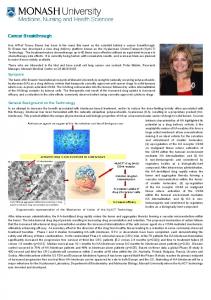
Table 6: Three contrasts as presented to the users On August 21st customers were 7.6 times more likely to purchase items from department 445 (MENSWEAR; Mens Nightwear) than they were on August 14th. They were bought in 2.2% of transactions on August 21st and 0.3% of transactions on August 14th. On August 14th customers were 6.3 times more likely to purchase items from department 855 (Girls Toys) and 851 (Boys Toys) than they were on August 21st. They were bought in 1.5% of transactions on August 14th and 0.2% of transactions on August 21st. On August 21st customers were 2.6 times more likely to purchase items from department 805 (Books) and 957 (Stationery) and 929 (Confectionery) than they were on August 14th. They were bought in 0.2% of transactions on August 21st and 0.1% of transactions on August 14th. Q 1. Is this rule surprising? Q 2. Is this rule potentially useful to the organization? Table 7 summarises the results of this investigation. We list the number of contrasts that were assessed as each surprising and potentially useful of those discovered by each system. As STUCCO’s filter penalises contrasts containing more elements, it is interesting to see whether the rules containing more departments that Magnum Opus found are assessed as less surprising or less potentially useful. For this reason, the table first presents the rules discovered by Magnum Opus grouped by the number of departments in the contrast, and then aggregated results for all rules. As previously discussed, all STUCCO contrasts contained only a single department. To our surprise, despite the greater selectiveness of the filter that it applies, a much lower proportion of the rules discovered by STUCCO were considered surprising by the retail experts. One possible explanation for this is that some of the Magnum Opus contrasts are actually spurious and hence are considered surprising because they do not actually have any basis in fact. To assess this possibility we performed chisquare tests of independence on all the contrasts and then a one-tailed homoscedastic t-test of the resulting probabilities of the surprising and the unsurprising rules. This test failed to find a significant difference in the chi-square probabilities of the two groups (t = 0.3788, p = 0.3097). To illustrate this apparent lack of inter-relationship between the probability that the antecedent and consequent are independent and the assessments of surprisingness, Figure 1 plots the chi-square test probabilities for each of the rules, with those rules identified as surprising distinguished from those that are not. Note that the x-axis is ordered by Magnum Opus’ output order, from highest to lowest leverage, an ordering correlated with chi-square test probabilities. The proportion of contrasts assessed as potentially useful are very similar between Magnum Opus and STUCCO. A chi-square test of independence indicates that the difference is not significant at the 0.05 level (χ2 = 0.0134, df=1, p =
Table 7: Summary of assessments System Magnum Opus Magnum Opus Magnum Opus Magnum Opus STUCCO
(1 Dept.) (2 Depts.) (3 Depts.) (All)
Total no rules 56 23 4 83 19
Surprising 12 (21%) 10 (43%) 1 (25%) 23 (28%) 2 (11%)
Potentially Useful 15 (27%) 5 (22%) 1 (25%) 21 (25%) 5 (26%)
Figure 1: Plot of surprising and not surprising contrasts by chi-square p
0.907). Considering the Magnum Opus rules with differing numbers of departments, the proportion drops slightly for the two department and three department contrasts. However, a chi-square test of independence indicates that this variation in proportions is not significant (χ2 = 0.2199, df=2, p = 0.896).
4.2
An assessment of negative conditions
As noted above, our assessment from comparing the three systems’ outputs was that C4.5rules had not identified many of the key contrasts. The system is not designed to perform this task and does not appear suited to the task. There are two striking differences between the rules produced by C4.5rules and those produced by the other systems. First, some of the rules identify relatively small differences in frequency between the two classes. This is presumably because they are introduced by the system in an attempt to find some form of discrimination between large numbers of cases that could not be covered by rules with greater discriminate performance. The second difference is that the rules produced by C4.5rules contain negative conditions. Because of the nature of the system there was no way to block this. As our prior expectation was that negative conditions would not be of value we configured both STUCCO and Magnum Opus to prevent them. Due to our strong expectations about the
likely outcomes and our desire to minimize the imposition on our industry collaborators we decided not to present the rules produced by C4.5rules for assessment of surprisingness and potential usefulness. Instead, we presented the set of rules and asked only for a simple assessment of whether the negative conditions were of potential value. The following is a fictitious example of such a rule in the format that we employed. On August 21 customers were 5.0 times more likely to purchase items from department 123 (INFANTS; Diapers) and nothing from department 345 (BEVERAGES; Beer) than they were on August 14. This occurred in 2.5% of transactions on August 21 and 0.5% of transactions on August 14. The response from our industry collaborators was that while negative conditions of these form were of potential value, these specific rules did not appear to be of interest and were more difficult to interpret than the Magnum Opus and STUCCO rules. This response is an interesting one. While it provides some support for our belief that classification rule discovery is not an appropriate approach to contrast discovery, it indicates that techniques that develop contrasts with negative conditions may be of value in at least this application. To develop useful techniques of this form may be quite a challenge, as straightforward application of either STUCCO or
Magnum Opus with negative conditions enabled produces sets of contrasts strongly dominated by negative conditions. This is because negative conditions have far greater cover than positive conditions and hence have greater potential to produce rules with strong effects. However, our intuition is that negative conditions will only be considered valuable in the current application when their effect is quite exceptional.
anonymous retail collaborators. We wish to thank Stephen Bay for supplying STUCCO and Christian Borgelt for supplying Apriori. We also greatly appreciate Stephen Bay’s constructive comments on an early draft of the paper. We are also grateful to John Crossley and Ying Yang for assistance with refining the presentation of our proof.
7.
5.
CONCLUSIONS
We set out to compare the performance of three alternative data mining techniques on a contrast-discovery task. To our surprise we discovered that the core contrast-setdiscovery task as defined by Eq. 1 is strictly equivalent to a special case of the more general rule-discovery task (Eq. 8). This in no way devalues the key contribution of Bay and Pazzani [2], which is the identification of contrast discovery as a new and valuable data mining task and the characterization of its requirements. From our study and analysis we reach the following conclusions about contrast analysis and identify the following issues as worthy of further investigation. First, the application of some form of filter to remove spurious correlations is important. The exact form that such a filter should take is, however, an area that is ripe for further research. Our investigation suggests that neither STUCCO nor Magnum Opus is applying a perfect filter. STUCCO seems to discard some contrasts of potential value. Magnum Opus appears to include some contrasts that are very probably spurious. However, in our study both systems were applied with default settings, and it is likely that tuning of their existing mechanisms to the specific task would result in better performance. It would be interesting to investigate in greater depth the issue of whether there is a substantial difference between the application of a chi-square test of independence and a binomial sign test as a filter. It would also be interesting to investigate further the relative merits of adjusting the statistical tests to allow for multiple comparisons. Our belief is that it is inadvisable to do so, because it will result in unacceptable type-two error. Rather, we should take account of the likelihood of type-one error in the assessment and investigations subsequent to the initial contrast-discovery process. Another issue revealed by our research is the need for appropriate methods to describe the contrasts that are discovered. It is clear that the traditional association-rule measures of support, confidence and lift are not directly appropriate. It is likely, however, that related measures would be useful. It would be valuable to study what information users find useful and how that information can be presented clearly and concisely. In summary, the current research has heightened our appreciation of the importance of contrast analysis. As our theorem proves, existing rule-discovery techniques can be applied to perform the core contrast-discovery task. However, it is possible that new techniques are required for filtering the contrasts that are considered potentially interesting. Finally, there is a need to develop appropriate methods for describing contrasts to end-users.
6.
ACKNOWLEDGMENTS We greatly appreciate enthusiasm and support of our
REFERENCES
[1] R. Agrawal, T. Imielinski, and A. Swami. Mining associations between sets of items in massive databases. In Proc. 1993 ACM-SIGMOD Int. Conf. Management of Data, pages 207–216, Washington, DC, May 1993. [2] S. D. Bay and M. J. Pazzani. Detecting group differences: Mining contrast sets. Data Mining and Knowledge Discovery, 5(3):213–246, 2001. [3] J. Bayardo, Roberto J. Brute-force mining of high-confidence classification rules. In Proc. Third Int. Conf. Knowledge Discovery and Data Mining (KDD-97), pages 123–126, Menlo Park, CA, 1997. AAAI Press. [4] J. Bayardo, Roberto J. Efficiently mining long patterns from databases. In Proc. 1998 ACM-SIGMOD Int. Conf. Management of Data, pages 85–93, 1998. [5] C. Borgelt. Apriori. (Computer Software) http://fuzzy.cs.Uni-Magdeburg.de/~borgelt/, February 2000. [6] S. H. Clearwater and F. J. Provost. RL4: A tool for knowledge-based induction. In Proc. of Second Intl. IEEE Conf. on Tools for AI, pages 24–30. IEEE Computer Society Press, 1990. [7] J. Davies and D. Billman. Hierarchical categorization and the effects of contrast inconsistency in unsupervised learning. In Proc. Eighteenth Annual Conf. Cognitive Science Society, page 750, 1996. [8] G. Dong and J. Li. Efficient mining of emerging patterns: Discovering trends and differences. In ACM SIGKDD 1999 Int. Conf. Knowledge Discovery and Data Mining, pages 15–18. ACM, 1999. [9] F. Provost, J. Aronis, and B. Buchanan. Rule-space search for knowledge-based discovery. CIIO Working Paper IS 99-012, Stern School of Business, New York University, New York, NY 10012, 1999. [10] J. R. Quinlan. C4.5: Programs for Machine Learning. Morgan Kaufmann, San Mateo, CA, 1993. [11] R. Rymon. Search through systematic set enumeration. In Proc. KR-92, pages 268–275, Cambridge, MA, 1992. [12] R. Segal and O. Etzioni. Learning decision lists using homogeneous rules. In AAAI-94, Menlo Park, CA, 1994. AAAI press. [13] G. I. Webb. OPUS: An efficient admissible algorithm for unordered search. Journal of Artificial Intelligence Research, 3:431–465, 1995. [14] G. I. Webb. Efficient search for association rules. In The Sixth ACM SIGKDD Int. Conf. Knowledge Discovery and Data Mining, pages 99–107, New York, NY, 2000. The Association for Computing Machinery. [15] G. I. Webb. Magnum Opus version 1.3. Computer software, Distributed by Rulequest Research, http://www.rulequest.com, 2001.