Abstract: We propose an estimation method for an errors-in-variables model with ... â¥2. F subject to. RR = Ip and R ËD = 0. (1) is the errors-in-variables (EIV) ... For dynamical systems a similar negative result is first ... order to make the EIV estimation problem with un- ..... In (Kukush et al., 2005), steps 2 and 3 of the algorithm.
14th IFAC Symposium on System Identification, Newcastle, Australia, 2006
ON ERRORS-IN-VARIABLES ESTIMATION WITH UNKNOWN NOISE VARIANCE RATIO I. Markovsky ∗ , A. Kukush ∗∗ , and S. Van Huffel ∗ ∗ ESAT,
SCD-SISTA, K.U.Leuven, Kasteelpark Arenberg 10, B-3001 Leuven, Belgium ∗∗ Kiev National Taras Shevchenko University, Vladimirskaya st. 64, 01033, Kiev, Ukraine
Abstract: We propose an estimation method for an errors-in-variables model with unknown input and output noise variances. The main assumption that allows identifiability of the model is clustering of the data into two clusters that are distinct in a certain specified sense. We show an application of the proposed method for system identification. Keywords: errors-in-variables, system identification, total least squares, clustering.
1. INTRODUCTION
EIV models with two or more unknown noise parameters, however, are unidentifiable by second order methods, i.e., there are many solutions that are not distinguishable from the second order statistics. This unidentifiability problem is well known in the context of the Frisch scheme (Frisch, 1934; De Moor, 1988). For dynamical systems a similar negative result is first proven in (Anderson, 1985).
Corresponding to the total least squares (TLS) problem �2 � {Rˆ tls , Dˆ tls } := argmin �D − Dˆ �F subject to R,Dˆ (1) RR� = I p and RDˆ = 0 is the errors-in-variables (EIV) model ˜ D = D¯ + D,
Various additional assumptions can be imposed in order to make the EIV estimation problem with unknown noise covariance structure identifiable. An overview of methods for EIV system identification is given in (Söderström et al., 2002; Söderström, 1981). In this paper we show a new assumption that allows to derive consistent parameter and noise variance estimates. The idea comes from (Wald, 1940), where a static single input single output (m = p = 1) EIV model is considered and the proposed estimator is the line passing through the mean values of two clusters of data points. We develop this simple idea for multi input single output static and dynamic EIV models. The key consistency assumption for the method is that the data D has as many clusters as there are unknown noise parameters. For example, the proposed method is not applicable for problems where the inputs are stationary, which is a typical assumption in much of the prior work on EIV system identification. Also in
¯ = row dim(D) − p =: m. (2) rank(D)
Here D¯ is a true value and D˜ is a measurement error that is modeled as a zero mean random matrix with independent and identically distributed (i.i.d.) elements. The TLS estimator (1) is maximum likelihood for the EIV model (2) if, in addition to the previous assumptions, the entries of D˜ i j are normally distributed. The variance of D˜ i j needs not be known, but the i.i.d. assumption is often too restrictive. More general EIV models, where the measurement errors need not be i.i.d., have been considered in (Kukush and Van Huffel, 2004). The corresponding TLS-type problems are called weighted TLS problems. A key assumption in this work is that the noise covariance structure, i.e., the covariance matrix of ˜ is known up to a scaling factor. One can argue vec(D) that the knowledge of the noise covariance structure up to a scalar is again restrictive in practice.
172
the dynamic case, we assume that the input and output measurement noises are white and uncorrelated.
of models that can not be represented in the form (3), however, is non-generic in Rq .
The assumption that the data can be clustered means that the true input changes character while the noise properties remain the same. This assumption can be viewed equivalently as having a set of data records from experiments with different true inputs. Such an assumption is certainly restrictive and presently we do not have specific applications in mind.
Corresponding to the representation (3) are the input/output partitionings of the data and measurement error matrices � � � � ˜ Di m ˜ =: Di m . and D D =: ˜ p Do Do p In Section 3 we use the input/output representation (3) and assign different noise variances to the input and output variables.
In Section 2 we describe kernel and input/output representations of static and dynamic linear models. Section 3 presents the proposed estimation method for static EIV models and states conditions for consistency. Section 4 extends the method to dynamic models and Section 5 shows simulation examples for EIV system identification. For simplicity the proposed method is applied to the special case of single output models and covariance structure known up to two unknown scalars: the input and the output noise variances. In the conclusions we discuss the extension of the method for problems involving more than two unknown parameters of the covariance matrix.
2.2 Dynamic models In the dynamic context the given data wd ∈ (Rq )T is a finite vector time series and the model is a subset of the data space (Rq )T . We consider linear time-invariant (LTI) models. The LTI model class admits a difference equation representation B(R) := { w ∈ (Rq )T | R0 w(t) + R1 w(t + 1) + · · · + Rl w(t + l) = 0, for t = 0, . . . , T − l }. (4) The matrices Ri ∈ Rg×q are parameters of the model. With g = 1 and Rl �= 0, B(R) is a single output model.
2. KERNEL AND INPUT/OUTPUT REPRESENTATIONS OF LINEAR MODELS
A given LTI model B generically admits an input/output representation � � � � u m � B= w= � P0 y(t) + P1y(t + 1) + · · · y 1 + Pl y(t + l) = Q0 u(t) + Q1u(t + 1) + · · · � + Ql u(t + l), for t = 0, . . . , T − l ,
2.1 Static models The data matrix D ∈ Rq×N has as rows the variables of interest and as columns the observed samples of those variables. A linear static model B for D is a subspace of Rq . Such a model can be represented as the kernel of a matrix R ∈ Rg×q , i.e.,
−1 � l � Pi ∈ R p×p , Qi ∈ R p×m , and ∑lk=0 Pk zk ∑k=0 Qk zk is a proper rational function (transfer function of B).
B = { d ∈ Rq | Rd = 0 } =: ker(R). In the numerical linear algebra literature, however, the input/output representation � � � � � di m � � B(X) := d = (3) � X di = do do p
3. STATIC PROBLEMS WITH ONE OUTPUT AND TWO UNKNOWN NOISE PARAMETERS
is preferred over the kernel one because it makes explicit the input/output structure of the model. The matrix X ∈ Rm×p , m+ p = q in B(X) is a parameter of the model. Note that while the parameter R in a kernel representation is in general non-unique, for a fixed input/output partitioning, the parameter X is unique.
First we consider the special case of EIV static model with one output and covariance structure known up to two scalars: input and output noise variances. This model corresponds to the classical linear system of equations Ax ≈ b with noises on A and b of unknown size. The model is unidentifiable without additional information on the noise covariance structure. For example, the weighted TLS method requires that the ratio of the input and output noise variances is known.
˜ such that R˜ R˜ � = I p Given R, one can always find R, ˜ and ker(R) = ker(R). Note that if R is full row rank, then the number of rows g := row dim(R) of R is equal to the number of outputs p of B = ker(R). In the single output case, RR� = �R�2 = 1, makes R unique.
Our assumption about the noise covariance matrix is that � � � � E D˜ i D˜ � E D˜ i D˜ � λ¯ iWi 0 � i o ˜ ˜ E DD = ˜ ˜ � =: 0 λ¯ oWo , (5) E D˜ o D˜ � i E Do Do
The first m variables di in the input/output representation (3) are inputs, i.e., they can be chosen freely. The last p variables do are outputs, i.e., they are fixed by the input and the model. The integers m and p are invariant of the representation. Note that not every model B ⊆ Rq admits an input/output representation with a fixed input/output partitioning. The set
where Wi ∈ Rm×m and Wo ∈ R are known positive definite matrices, and λ¯ i (the input variance) and λ¯ o (the output variance) are unknown positive scalars.
173
If the minimal singular value of D1i (D1i )� − D2i (D2i )� is separated from zero, the problem of estimating simultaneously λo , μ , and R is identifiable (see Theorem 1 below). This condition is related to the existence ¯ Correspondingly the of clusters in the true data D. clustering problem is �
� � � min �λ j D1i (D1i )� − D2i (D2i )� � , max
Provided that the smallest eigenvalue of the sample covariance matrix DD� has multiplicity one (the generic case), the TLS solution Rˆ tls is unique and is given by the eigenvector of DD� , corresponding to the smallest eigenvalue. Alternatively, we are looking for a solution R to the nonlinear system of equations R(DD� − λ I) = 0 corresponding to the smallest value of λ .
permutation matrix Π
(8) where λ1 (A), . . . , λdim(A) (A) are the eigenvalues of A.
The TLS solution corresponds to an EIV model, in which the input/output noise variance ratio λ¯ i /λ¯ o =: μ¯
The estimation problem corresponding to (7) is more complicated than a generalized eigenvalue/singular value decomposition: we need to find a common generalized eigenvalue-eigenvector pair for two pairs of symmetric positive semidefinite matrices that depend on a scalar parameter. In general, (7) has no exact solution, so that an approximation is needed.
is equal to one, {D˜ i,i j } are i.i.d., and {D˜ o,i j } are i.i.d. The case of a known noise ratio μ¯ �= 1, corresponds to a weighted TLS problem, which seeks for a solution to the system ��
� μ¯ Im 0 = 0, R DD� − λo 0 1
We propose the following nonlinear least squares type approximate solution: � 2 � μˆ = argmin λo1 − λo2 + C sin2 ∠(R1 , R2 ) , (9)
corresponding to the smallest value of λo . The numerical solution in this case is performed via the generalized eigenvalue or singular value decomposition (instead of the ordinary eigenvalue or singular value decomposition).
μ
where (λok , Rk ) is the minimal � generalized eigenvalue eigenvec. pair of the pencil Dk (Dk )� , diag(μ Wi ,Wo ) , C is a regularization parameter, and ∠(R1 , R2 ) stands for the angle between the vectors R1 and R2 . The first term in the cost function makes both eigenvalues close to each other, while the second term makes the corresponding eigenvectors close to each other. The regularization parameter C allows to turn the two objectives optimization problem into a one objective optimization. Our experience is that the results are rather insensitive to the value of this parameter and in the simulation examples of Section 5 we set C = 1.
�
� μ Wi 0 , W (μ ) := 0 Wo so that E D˜ D˜ � = λ¯ oW (μ¯ ). Corresponding to the EIV model and assumption (5) is the weighted TLS problem � �2 � ˆ � subject to RDˆ = 0, min �W −1/2 (μ¯ )(D − D) � Denote
ˆ R,D
j=1,...,m
F
or equivalently the nonlinear system of equations
(6) R DD� − λoW (μ¯ ) = 0,
Once the optimal estimate μˆ of the noise variance ratio μ is found, the estimation problem becomes a classical generalized TLS problem. In summary, the proposed estimation procedure has three stages.
where again the true input/output noise ratio μ¯ is assumed known. The computation can be carried out via a generalized eigenvalue or singular value decomposition. In the literature the estimator for this case is called generalized TLS (Van Huffel and Vandewalle, 1989).
1. Cluster the data by solving (8). 2. Compute the noise variance ratio estimate μˆ by solving (9) for the clusters identified on step 1. 3. Solve the standard generalized TLS problem for the estimated value of μ on step 2.
Now consider the problem of unknown true noise ratio μ¯ . Even if R is properly normalized, e.g., �R� = 1, a solution to (6) is non-unique. This is a manifestation of a lack of identifiability of the model with unknown input and output noise variances. We propose to resolve the unidentifiability problem by considering a system of two independent estimating equations. After a permutation of the columns of D via a permutation matrix Π, define � 1 2� � 1 2� D D m DΠ =: D D =: i1 i2 Do Do 1
The clustering problem (8) has combinatorial complexity, so that (except for small examples) it can be solved only via heuristic methods. See (Xu and Wunsch, 2005) for a survey of clustering algorithms. In our simulation examples we use the K-means algorithm implemented in the Statistics Toolbox of M ATLAB.
(7)
The optimization problem on step 2 is a rather simple one because it involves a single scalar decision variable and the search interval is lower bounded by 0. Note that each cost function evaluation involves two generalized singular value decompositions.
corresponding to the two parts D1 and D2 of the data matrix.
The procedure described above is closely related but not equivalent to the one of (Kukush et al., 2005).
and consider two copies of (6)
R Dk (Dk )� − λoW (μ ) = 0,
for k = 1, 2,
174
In (Kukush et al., 2005), steps 2 and 3 of the algorithm are different.
becomes the structured system of equations RHl+1 (w) = 0,
2’. Compute the noise variance estimates λˆ i and λˆ o by solving the optimization problem � ��� ��2 � μ1 � � 2 1 2 min � 2 � + C sin ∠(R , R ) , (9’) λi ,λo � μ �
(10)
where Hl+1 (w) is the block-Hankel matrix with l + 1 block rows, constructed from the time series w: ⎤ ⎡ w(1) w(2) ··· w(T − l) w(3) ··· w(T − l + 1)⎥ w(4) ··· w(T − l + 2)⎥ ⎥, .. .. ⎦ . . . w(l + 1) w(l + 2) ··· w(T )
⎢ w(2) ⎢ Hl+1 (w) := ⎢ w(3) ⎣ ..
where μ k and Rk are respectively the smallest eigenvalue and corresponding eigenvector of
(11)
and
Dk (Dk )� − diag(λiWi , λoWo ).
� � R := R0 R1 · · · Rl . With noisy data wd and T > q(l + 1) + l, generically (4) is not compatible, so that an approximation is needed.
3’. Define the estimate Rˆ as the eigenvector corresponding to the smallest eigenvalue of the matrix DD� − diag(λˆ iWi , λˆ oWo ).
The structured TLS problem is the dynamic equivalent of the TLS problem (1):
Problem (9) can be viewed as a modification of (9’). In general both problems are nonconvex and nonsmooth, however, (9) is univariate while (9’) is bivariates and for this reason more difficult to solve. The estimator on Step 3’ is called the adjusted least squares. It is equivalent to the generalized TLS estimator on step 3 with μˆ = λˆ i /λˆ o .
ˆ 2 min �w − w� R,wˆ
subject to RR� = 1, and RHl+1 (w) ˆ = 0. (12)
Its solution however can not be expressed in closed form via a singular value decomposition of the data matrix as in the static case and needs nonlinear optimization methods (Markovsky et al., 2004).
Statistical consistency of the estimator using steps 2’ and 3’ is proven in (Kukush et al., 2005). Here we state the main result, specialized for the considered problem. (The result of (Kukush et al., 2005) applies to multi input multi output dynamic problems as well.)
The structured TLS problem (12) corresponds to the ˜ where w¯ is a trajectory of EIV model wd = w¯ + w, ¯ for some R¯ ∈ R1×q(l+1) , and w˜ is a white random B(R) sequence with covariance matrix that is equal to a multiple of the identity. If in addition the measurement errors w˜ are normally distributed, the structured TLS estimator is maximum likelihood.
Theorem 1. Assume that: i). there exists δ > 0, such that E |D˜ i j |4+δ are uniformly bounded for all i, j ii). N11 �D¯ 1i �F and N12 �D¯ 2i �F are bounded, where N1 := col dim(D1 ) and col dim(D2 ) � 1 N12 := 1� > 0, iii). lim infN1 ,N2 →∞ σmin N1 Di Di − N12 D2i D2� i where σmin (A) is the smallest singular value of A, iv). lim infN1 →∞ N11 trace(X �Wi X) > 0 lim infN2 →∞ N12 trace(Wo ) > 0, and � v). lim infNk →∞ N1 σmin D¯ ki (D¯ ki )� > 0, for k = 1, 2.
More general weighted structured TLS problems allow to take into account the noise covariance matrix that is known up to a scaling factor. As in the static case, dynamic EIV problems in which the covariance structure is specified up to more than one scaling factor are unidentifiable. Next we consider the case when the noise covariance matrix is known up to two scalars—the input and output noise variances. Accordingly, � � � � � λ¯ i Im 0 μ¯ Im 0 ¯ = λo =: λ¯ oW (μ¯ ). cov w(t) ˜ = 0 1 0 λ¯ o (13) Let W(μ ) := diag(W (μ ), . . . ,W (μ )). �� � �
k
¯ as N1 , N2 → ∞, Then λˆ i → λ¯ i , λˆ o → λ¯ o , and Xˆ → X, almost surely.
4. APPLICATION FOR DYNAMIC MODELS Certain system identification problems can be posed as structured TLS problems (Markovsky et al., 2005a). The main difference with the static TLS problem (1) is that now the data matrix is block-Hankel structured. For application of the structured TLS method, however, the measurement error covariance structure should be known up to a scaling factor. In this section we address a dynamic version of the problem of Section 3.
T times
The weighted structured TLS problem corresponding to the EIV model with the noise covariance (13) is ˆ � W−1 (μ¯ ) (wd − w) ˆ min (wd − w) R,wˆ
RR� = 1,
subject to
RHl+1 (w) ˆ = 0. (14)
However, this problem can be solved only for a given parameter μ¯ .
Written in a matrix form the difference equation
In (Markovsky et al., 2005b; Markovsky and Van Huffel, 2005) we show that the structured TLS problem
R0 w(t) + R1w(t + 1) + · · · + Rl w(t + l) = 0,
175
is generically equivalent to the following nonlinear weighted least squares problem � � � � � X −1 � min X −1 Hl+1 (wd )Γ (X, μ¯ )Hl+1 (wd ) −1 X (15) where Γ(X, μ¯ ) is a block banded and Toeplitz matrix that depends on X and W(μ¯ ). In turn the optimization problem (15) can be seen equivalently as a least squares approximate solution method for the nonlinear system of equations � � � X −1 Hl+1 (wd )Γ−1/2 (X, μ¯ ) = 0.
5. SIMULATION EXAMPLE Consider the EIV model (2). The covariance structure of the measurement errors D˜ is known up to scaling factors (the true noise variances) λ¯ i and λ¯ o . The simulation example aims to show consistency of the ¯ estimators for the unknown parameters λ¯ i , λ¯ o , and X, the parameter in an input/output representation of the ¯ true model that has generated the data D. Let UN (l, u) be a matrix with N columns, composed of independent and uniformly distributed random variables in the interval [l, u]. The true values D¯ i and R¯ are selected as follows: � � � � D¯ i = UN (−0.5, 0.5) UN (10, 20) , X¯ � = 1 1 ,
In order to resolve the identifiability problem, we make the assumption that the true time series w¯ changes its behavior at time T , i.e., the time series
where N is varied from 10 to 500. Correspondingly D¯ o := X¯ � D¯ i . Note that we artificially create two clus¯ In this ters (the first N and the last N columns of D). simulation example the K-means clustering algorithm detects without errors the two clusters. The measurement errors are zero mean, independent, normally distributed with variances λi = 0.01 and λo = 0.04.
w¯ 1 := (w(1), ¯ . . . , w(T ¯ )) has different mean and dispersion than the time series ¯ + 1), . . ., w(T ¯ )). w¯ 2 := (w(T This assumption corresponds to the clustering assumption in the static case. Note that now the ordering of the data samples corresponds to time, so that we can not permute them as in the static case.
With this simulation setup we apply the proposed estimation method and average the results for 500 noise realizations. The average values of the noise variance estimates λˆ i and λˆ o are shown on Figure 1.
Under the existence of clusters, define w1d , w2d analogously to w¯ 1 , w¯ 2 , and consider the system of two nonlinear equations � � � Xk −1 Hl+1 (wkd )Γ−1/2 (X, μ ) = 0, for k = 1, 2. (16) For noise free data, the equations have a common solution X 1 = X 2 = X¯ and μ = μ¯ . In the presence of noise, an approximate solution is needed and we propose the same criterion as in the static case � 2 � μˆ = arg min λo1 − λo2 + C sin2 ∠(R1 , R2 ) , (17)
Figure 2 shows the average relative estimation error e :=
1 500 �X¯ − Xˆ (k)� , ∑ �X� ¯ 500 k=1
where Xˆ (i) is the estimate of the parameter X¯ in the ith repetition of the experiment. 0.012
μ
where Rk and λok come from the structured TLS problems associated with (16), � � Rk := (X k )� −1 ,
0.01
λˆ i
0.008
and
0.006 0.004
λok
:= R
k
� Hl+1 (wkd )Γ−1 (X, μ )Hl+1 (wkd )(Rk )� .
0.002
Each cost function evaluation involves solving two structured TLS problems.
0
In summary, the algorithm for the considered EIV identification problem is:
100
200
100
200
N
300
400
500
300
400
500
0.048 0.047
T
0.046
1. Detect a time instant at which wd changes its behavior. 2. Solve the optimization problem (17) for the partitioning of the data found in step 1, and 3. Solve the structured TLS problem (14) for the estimated value μˆ in step 2.
λˆ o
0.045 0.044 0.043 0.042 0.041 0.04
Note 1. The cost functions in (9), (9’), and (17) are discontinuous. Therefore, the global minimum might not exist. The minimization is performed up to certain tolerance that decreases to zero, as the number of observations increases.
N
Fig. 1. Average values of the noise variance estimates λˆ i and λˆ o as a function of half the sample size N . The dashed lines are the true values.
176
Control: Computation, Identification and Modelling’); EU: PDTCOIL, BIOPATTERN, ETUMOUR.
0.016 0.014 0.012
REFERENCES
e
0.01 0.008
Anderson, B. (1985). Identification of scalar errorsin-variables models with dynamics. Automatica 21, 625–755. De Moor, B. (1988). Mathematical concepts for modeling of static and dynamic systems. PhD thesis. Dept. EE, K.U.Leuven, Belgium. Frisch, R. (1934). Statistical confluence analysis by means of complete regression systems. Technical Report 5. Univ. of Oslo, Economics Institute. Kukush, A. and S. Van Huffel (2004). Consistency of elementwise-weighted total least squares estimator in a multivariate errors-in-variables model AX = B. Metrika 59(1), 75–97. Kukush, A., I. Markovsky and S. Van Huffel (2005). Estimation in a linear multivariate measurement error model with clustering in the regressor. Technical Report 05–170. Dept. EE, K.U.Leuven. Markovsky, I. and S. Van Huffel (2005). Weighted structured total least squares. Technical Report 05–41. Dept. EE, K.U.Leuven. Markovsky, I., J. C. Willems, S. Van Huffel, B. De Moor and R. Pintelon (2005a). Application of structured total least squares for system identification and model reduction. IEEE Trans. on Aut. Control 50(10), 1490–1500. Markovsky, I., S. Van Huffel and A. Kukush (2004). On the computation of the structured total least squares estimator. Num. Lin. Alg. with Appl. 11, 591–608. Markovsky, I., S. Van Huffel and R. Pintelon (2005b). Block-Toeplitz/Hankel structured total least squares. SIAM J. Matrix Anal. Appl. 26(4), 1083–1099. Söderström, T. (1981). Identification of stochastic linear systems in presence of input noise. Automatica 17(5), 713–725. Söderström, T., U. Soverini and K. Mahata (2002). Perspectives on errors-in-variables estimation for dynamic systems. Signal Processing 82, 1139– 1154. Van Huffel, S. and J. Vandewalle (1989). Analysis and properties of the generalized total least squares problem AX ≈ B when some or all columns in A are subject to error. SIAM J. Matrix Anal. 10(3), 294–315. Wald, A. (1940). The fitting of straight lines if both variables are subject to error. Ann. Math. Stat. 11, 284–300. Xu, R. and D. Wunsch (2005). Survey of clustering algorithms. IEEE Trans. on Neural Networks 13(3), 645–678.
0.006 0.004 0.002 0
100
200
300
400
500
N
Fig. 2. Relative error of estimation e as a function of half the sample size N . 6. CONCLUSIONS We have considered an EIV estimation problems for single output static and dynamic systems, with measurement error covariance matrix known up to two unknown parameters. The model is identifiable under the assumption that the data has two clusters that are distinct in a specified sense. The proposed estimation method has three steps: cluster the data, solve a univariate optimization problem for the noise variance ratio, solve a standard TLS-type problem for the estimated noise variance ratio. In the static case the cost function evaluation on the second step involves solving a couple of generalized TLS problems and in the dynamic case it involves solving a couple of weighted structured TLS problems. Identifiability of the model is recovered by constructing two estimating equations corresponding to the two clusters. The idea generalizes to problems involving more than two unknown parameters in the measurement error covariance matrix. As many clusters and corresponding estimating equations are needed as there are unknown covariance parameters. The estimation procedure in this case, however, requires solving a multidimensional optimization problem on the second step. It is an open problem what special properties (if any) this optimization problem has and how to exploit them in effective EIV estimation algorithms.
ACKNOWLEDGEMENTS I. Markovsky is a postdoctoral researcher and S. Van Huffel is a full professor at the K.U.Leuven, Belgium. A. Kukush is a full professor at the Kiev National Taras Shevchenko Univ., Ukraine. We are grateful to Prof. H. Schneeweiss for fruitful discussions. Prof. Kukush is supported by a senior postdoctoral fellowship from the Dep. of Applied Economics of the K.U.Leuven. Our research is supported by Research Council KUL: GOA-AMBioRICS, GOAMefisto 666, several PhD/postdoc & fellow grants; Flemish Government: FWO: PhD/postdoc grants, projects, G.0078.01 (structured matrices), G.0407.02 (support vector machines), G.0269.02 (magnetic resonance spectroscopic imaging), G.0270.02 (nonlinear Lp approximation), G.0360.05 (EEG signal processing), research communities (ICCoS, ANMMM); IWT: PhD Grants; Belgian Federal Science Policy Office IUAP P5/22 (‘Dynamical Systems and
177