Dec 1, 2008 - On Errors-In-Variables Regression with Arbitrary Covariance and its. Application to ... tivariate polynomial which can, in principle, be carried out.
On Errors-In-Variables Regression with Arbitrary Covariance and its Application to Optical Flow Estimation Bj¨orn Andres, Claudia Kondermann, Daniel Kondermann, Ullrich K¨othe, Fred A. Hamprecht, Christoph S. Garbe Interdisciplinary Center for Scientific Computing, University of Heidelberg Abstract
of A and b, the linear additive Gaussian errors-in-variables (EIV) model (A, b, Σ) is specified by the following assumptions:
Linear inverse problems in computer vision, including motion estimation, shape fitting and image reconstruction, give rise to parameter estimation problems with highly correlated errors in variables. Established total least squares methods estimate the most likely corrections Aˆ and ˆb to a given data matrix [A, b] perturbed by additive Gaussian ˆ b+ noise, such that there exists a solution y with [A + A, ˆb]y = 0. In practice, regression imposes a more restrictive constraint namely the existence of a solution x with ˆ = [b + ˆb]. In addition, more complicated corre[A + A]x lations arise canonically from the use of linear filters. We, therefore, propose a maximum likelihood estimator for regression in the general case of arbitrary positive definite ˆ ˆb and x can be found covariance matrices. We show that A, simultaneously by the unconstrained minimization of a multivariate polynomial which can, in principle, be carried out by means of a Gr¨obner basis. Results for plane fitting and optical flow computation indicate the superiority of the proposed method.
(a) There exist latent variables Al ∈ Rm×n , bl ∈ Rm and additive errors in variables Ae ∈ Rm×n , be ∈ Rm such that A = Al + Ae and b = bl + be . (1) (b) Let vec([Ae , be ]) denote the column-wise vectorization of the composite matrix [Ae , be ]. Then the errors Ae , be are realizations of a random matrix A�e and a random vector b�e whose entries are normally distributed with zero mean and covariance matrix Σ vec([A�e , b�e ]) ∼ N (0, Σ) , i.e. (2) � � 2 exp − 12 �vec([Ae , be ])�Σ � . P (vec([Ae , be ])) = (2π)mn+m det Σ (3) with �·�Σ : Rmn+m → R+ 0 such that √ (4) ∀v ∈ Rmn+m : �v�Σ := v T Σ−1 v , which denotes the Mahalanobis norm for given Σ.
1. Introduction
(c) The latent vector bl linearly depends on the columns of Al , i.e. (5) ∃x ∈ Rn : Al x = bl ,
Linear inverse problems in computer vision, including motion estimation, shape fitting and image reconstruction, give rise to parameter estimation problems with highly correlated errors in variables. In this section, we introduce the statistically appropriate model for this context. We discuss related work in section 2 and introduce a new estimator allowing for arbitrary correlations in the data in section 3. Comparative results for plane fitting as well as for optical flow estimation are given in section 4, and conclusions are offered in section 5.
making this system of equations solvable. Under the assumption of the above EIV model, the maximum likelihood estimates Aˆe , ˆbe of A�e , b�e are the most likely (w.r.t. eq. (3)) errors such that conditions (a) and (c) are fulfilled. The solution x ˆ to the linear system (5) then follows from (A − Aˆe )ˆ x = b − ˆbe which is solvable due to (a) and (c). For an observed A,b the maximum likelihood estimation (MLE) of Al and bl hence reduces to the optimization problem
1.1. Errors-In-Variables Model Given noisy variables A ∈ Rm×n , b ∈ Rm , m, n ∈ N as well as a symmetric positive definite matrix Σ ∈ R(mn+m)×(mn+m) modeling the covariance of the entries
subject to
argmax P (vec([Ae , be ]))
(6)
= b − be .
(7)
Ae ∈Rm×n ,be ∈Rm ∃x ∈ Rn : (A − Ae )x
1
978-1-4244-2243-2/08/$25.00 ©2008 IEEE
Authorized licensed use limited to: IEEE Xplore. Downloaded on December 1, 2008 at 08:43 from IEEE Xplore. Restrictions apply.
10
10
10
20
20
20
30
30
30
40
40
40
50
50
50
60
60
60
70
70
80
−0.01
70 80
80 20
40
0
60
0.01
80
0.02
20
40
0
60
0.5
20
80
1
0
40
0.5
60
80
1
Figure 1. Locally constant optical flow estimation from 3 × 3 × 3 neighborhoods is considered. Left: Covariance matrix Σ ∈ R81×81 of the vectors vec([∂x g, ∂y g, ∂t g]), with structure owing to impulse response masks of linear derivative operators. Middle: Covariance matrix of ETLS equilibration vec(WL [∂x g, ∂y g, ∂t g]WRT ). Right: Unity matrix.
Due to the strict monotonicity of the exponential function in (3), the objective in (6) can be replaced by argmin �vec([Ae , be ])�Σ .
Ae ∈Rm×n ,be ∈Rm
(8)
An in-depth discussion of EIV models can be found in [12, 15].
2. Related Work This section addresses methods that solve related problems and differ from the estimator proposed in section 3 in either the objective function or the constraint. Given noisy variables A ∈ Rm×n , b ∈ Rm , the total least squares (TLS) estimator [16] is defined as argmin �vec([Ae , be ])�Imn+m
Ae ∈Rm×n ,be ∈Rm
(9)
subject to ∃y ∈ Rn+1 : [A − Ae , b − be ]y = 0 and �y�2 = 1 , (10) where Imn+m denotes the identity matrix of the indicated size. In fact, the Mahalanobis norm �vec([Ae , be ])�Imn+m equals the Frobenius norm of the matrix [Ae , be ]. Thus, TLS seeks the Frobenius minimal additive correction [Ae , be ] to [A, b] such that the matrix [A − Ae , b − be ] becomes rank deficient. If [A, b] results from perturbance of [Al , bl ] by independent and identically distributed Gaussian noise with zero mean, then TLS is the MLE of [Ae , be ] under the rank deficiency constraint [16]. The estimator we propose differs from TLS in two aspects: First, according to (2), we allow for arbitrary non-singular correlations in the errors. Second, we impose the constraint (5) instead of (10) stating that precisely the vector b − be is supposed to be a linear combination of the columns of A − Ae . This corresponds to a restriction of the TLS formulation, where rank deficiency only requires the columns of [A − Ae , b − be ] to be linearly
dependent. We thereby directly address linear regression problems, whereas TLS is in fact a subspace estimator. Subspace estimation with arbitrary covariance is comprehensively discussed in [6, 11]. Under the restrictive assumption that the columns of the matrix [A, b] are uncorrelated, subspace estimation can be reduced to TLS by weighting as detailed in [12, 17]. Our approach differs in that we consider regression rather than subspace estimation and in that we directly address polynomial minimization. From the wide range of subspace estimators, we compare directly against equilibrated TLS (ETLS) which was introduced in [13] and has been applied in computer vision, e.g. in [1]. ETLS aims at linearly transforming the system [A, b] such that the errors become approximately uncorrelated with equal variance. To this end, orthogonal matrices WL ∈ Rm×m , WR ∈ R(n+1)×(n+1) are employed, such that [A� , b� ] := WL [A, b]WRT . (11) Then TLS is performed on [A� , b� ] (yielding a solution y � ∈ Rn+1 ), and finally y := WR y � is understood as a solution to the initial problem. M¨uhlich and Mester [13] derive by the perturbation theory of eigenvectors [8] conditions on WL and WR , from which these matrices can be computed iteratively for arbitrary covariance. The benefit of mapping such estimation problems with arbitrary covariance to TLS is that the Eckart-Young Theorem [7] for matrix approximation allows for efficient and numerically stable TLS estimation by means of the singular value decomposition (SVD) [16]. However, ETLS is only an approximation to true MLE in case of highly structured covariance matrices. In order for ETLS to be the MLE, the covariance matrix of vec(WL [A, b]WRT ) has to equal the identity matrix. However, � � cov vec(WL [A, b]WRT ) =
(WR ⊗ WL )cov(vec([A, b]))(WR ⊗ WL )T (12)
where ⊗ denotes the Kronecker product. Due to the structure of the matrix (WR ⊗ WL ), covariance matrices cov(vec([A, b])) exist such that WL and WR cannot be chosen to equilibrate them. An example of remaining correlation after ETLS equilibration is shown in figure 1. Nevertheless, the results reported below support ETLS as an efficient approximation to MLE.
3. Maximum Likelihood Estimator In order to account for arbitrary covariance in the regression setting defined by the constraint (7), we propose to consider the objective function (8) and substitute for be according to (7) yielding argmin p(d) ,
d∈Rmn+n
Authorized licensed use limited to: IEEE Xplore. Downloaded on December 1, 2008 at 08:43 from IEEE Xplore. Restrictions apply.
(13)
m×n with p : Rmn+n → R+ ∀x ∈ Rn : 0 such that ∀Ae ∈ R
p(vec([Ae , x])) = �vec([Ae , b − (A − Ae )x])�Σ . (14) The objective function p is a multivariate polynomial in the unconstrained entries of Ae and x. The largest exponent of any of the free variables is two while (mixed) terms of order one through four occur. Depending on A, b, and Σ, this polynomial may be non-convex. However, there exists ˆ equals the finite a finite vector dˆ ∈ Rmn+n for which p(d) global minimum of this polynomial. This property is inherited from the Mahalanobis norm. In the following, we will use the abbreviation MR for the proposed maximum likelihood estimator, which stands for Mahalanobis regression.
3.1. Polynomial Minimization We have reduced the problem of finding maximum likelihood estimates for the corrections [Ae , be ] to the minimization of a multivariate polynomial p. We now describe a numerical minimizer for p. Furthermore, we will show how Gr¨obner bases can be used to reduce the problem of multivariate polynomial minimization to univariate polynomial root finding. 3.1.1
Numerical Minimization
The multivariate polynomial to be minimized can easily be differentiated algebraically. Hence, the first two terms of the Taylor approximation of p, namely, the gradient and the Hessian, are readily available. This suggests the use of a trust region method for optimization [5]. We therefore apply the large-scale optimization routine of Matlab which employs a subspace trust region method based on the interior-reflective Newton method described in [4]. This method first estimates a two-dimensional subspace based on the gradient and the Hessian matrix. The latter is inverted by means of preconditioned conjugate gradients. Then, the resulting minimization problem is solved by a Newton step. A host of alternative minimization techniques exists. Since ∂2 the second partial derivatives ∂x 2 p are linear in xj , their j roots can be evaluated efficiently. Thus, especially the cyclic coordinate descent method, which iteratively minimizes the polynomial with respect to each variable in turn, appears interesting. 3.1.2
Algebraic Minimization
In this section, we propose an algebraic approach to the minimization of the polynomial. Due to complexity, we have tested this approach only for small examples not included in this paper. We nevertheless point out the importance of this approach, which is due to the following reasons. First, the iterative numerical minimization of the multivariate polynomial is computationally expensive and
prone to convergence to local minima if p is non-convex. Second, depending on the application, p may need to be minimized multiple times for equal covariance Σ but different data A,b such as is the case with optical flow estimation from patches of an image sequence. Third, Σ may arise from only a small number of coefficients induced by linear filters. These three reasons taken together motivate the use of as much symbolic computation as possible in order to support the minimization process. Hence, in order to minimize the polynomial p over the ring of polynomials R[x1 , ..., xn ] in n ∈ N indeterminates, we differentiate the polynomial algebraically with respect to all indeterminates and obtain the following system of equations S = {p1 (x1 , ..., xn ) = 0, ..., pn (x1 , ..., xn ) = 0} . (15) This system can be solved by means of a Gr¨obner basis [3]. Let I = p1 , ..., pn , n ∈ N denote the ideal generated by the polynomials p1 , ..., pn . A Gr¨obner basis is a special basis of I for which root-finding is simpler than for the original system of equations. This is due to the elimination property of Gr¨obner bases, from which follows that for j ∈ Nn a basis polynomial in only j indeterminates exists. This means that one can successively find all the solutions of the system of equations by means of root-finding of univariate polynomials. The computation of a Gr¨obner basis can be carried out using Buchberger’s algorithm [3]. However, since this algorithm has exponential complexity in the worst case, it may be impractical even for relatively small problems if there is little structure in the covariance matrix. However, despite this complexity one should consider the computation of Gr¨obner bases as a preprocessing step due to the observations mentioned above.
4. Results In order to investigate the performance of the proposed estimator, we have applied the trust region method described above for the minimization of the multivariate polynomial (with ETLS initialization), first to the problem of fitting planes to point clouds with randomly and systematically correlated Gaussian noise (sections 4.1 4.2), and second to optical flow estimation where the covariance matrix is derived from the derivative filters applied to the image sequence (section 4.3).
4.1. Random Correlation The plane fitting problem in 3d-space amounts to solving an over-determined linear system of equations Ax = b, A ∈ Rm×2 , b ∈ Rm , x ∈ R2 approximately. In order to obtain test examples, we randomly choose the matrix Al and the parameter vector x and compute the vector
Authorized licensed use limited to: IEEE Xplore. Downloaded on December 1, 2008 at 08:43 from IEEE Xplore. Restrictions apply.
bl = Al x. To generate correlated additive Gaussian noise, we first choose a matrix L : R3m×3m → R with uniformly distributed entries within the range [0, 1]. Then, to perturb the latent data [Al , bl ], we generate uncorrelated Gaussian noise D ∈ Rm×3 with given standard deviation σ ∈ R and compute the noisy variables by vec([A, b]) = vec([Al , bl ]) + L vec(D)
(16)
Linear Mapping
Error box plot 0.9 4
(17)
To minimize the polynomial we employ the algorithm described in section 3.1.1. As initialization we use the result of the ETLS estimator. To test our algorithm for the plane fitting problem we consider eight different signal to noise ratios (SNR) between 100 and 0.5. For each SNR we solve 100 randomly generated plane fitting problems (as described above) for m = 8 points. The error is computed according to (17) for each plane fitting problem instance. To evaluate our method we investigate the distribution of the errors for each SNR separately. In Figure 2 we compare the results of our algorithm to those obtained by TLS and ETLS. The results indicate that for every noise level the quality of the proposed MR method is far superior to the TLS solution and superior to the ETLS solution.
4.2. Systematic Correlation We consider the same setting as in 4.1 except for the fact that we introduce stronger systematic correlation between the points by setting some entries of the mapping L manually. Figure 3 shows an example for a linear mapping, which induces systematic correlations of the noise, the corresponding covariance matrix and error box plots for the TLS, ETLS and MR method for a SNR of 10. The MR method again clearly outperforms the TLS method and is superior to the ETLS method due to its lower quantiles. The results indicate the superiority of the MR method for systematically correlated Gaussian noise.
4.3. Optical Flow Estimation Let N ∈ N and g ∈ R be a vector of all gray values in a sequence of images such that any j ∈ {1, . . . , N } uniquely indicates a pixel in the sequence. Moreover, consider linear shift invariant filters with finite impulse response which approximate partial derivatives of the signal in the two spatial as well as in the temporal directions [14]. Then, the approximate derivatives ∂x g, ∂y g, ∂t g ∈ Rm of a spatio-temporal N
0
0.7
í�
0.6
í� Covariance matrix
Then, the covariance matrix of the Gaussian distribution of vec([A, b]) follows from Σ = σ 2 LLT . The error for each of these plane fitting problems is computed as the norm of the difference vector between the estimated solution x ˆ and the true solution x. e := �ˆ x − x�2
0.8
2
0.5 í3
x 10
0.4
3
0.3
2
0.2
1 0
0.1 0
TLS
ETLS
MR
Figure 3. Results for a randomly chosen plane fitting problem in 3d-space with partially strongly correlated noise with SNR=10, left: linear mapping L for noise correlation and resulting covariance matrix C, right: error box plot for TLS, ETLS and MR
patch of size m of the sequence are obtained by matrices Lx , Ly , Lt ∈ Rm×N , defined by the filter coefficients, according to ∂x g = Lx g,
∂y g = Ly g,
∂t g = Lt g .
(18)
Suppose now the existence of latent gray values gl ∈ RN and errors ge ∈ RN which are realizations of random variables distributed according to N (0, Σg ), such that g = gl + ge . The covariance matrix Σg may, for instance, be obtained from camera calibration measurements. Then, the brightness change constraint equation (BCCE) for locally constant displacement [10, 2] imposes the existence of optical flow fx , fy ∈ R which is constant with respect to the chosen patch, i.e. (∂x gl )1 (∂y gl )1 (∂t gl )1 � � fx .. .. .. = − . . . . fy (∂x gl )k (∂y gl )k (∂t gl )k
� �
� � Al
bl
(19) Note that A, Ae ∈ Rm×2 and b, be ∈ Rm can be defined by replacing gl by g and ge , respectively, in eq. (19). Statistically appropriate motion estimation now means solving the EIV problem (A, b, Σ) with Σ
= =
cov(vec([A, b])) Lx Σg LTx Lx Σg LTy Ly Σg LTx Ly Σg LTy Lt Σg LTx Lt Σg LTy
Lx Σg LTt Ly Σg LTt .(20) Lt Σg LTt
A covariance matrix for optical flow estimation from 3 × 3 × 3 neighborhoods is shown in the first graph of Figure 1. Since the linear filters induce correlated Gaussian noise with the non-block-diagonal covariance matrix (20) in the
Authorized licensed use limited to: IEEE Xplore. Downloaded on December 1, 2008 at 08:43 from IEEE Xplore. Restrictions apply.
−3
7
SNR=100
x 10
SNR=50
SNR=20
SNR=10
0.014
0.035
0.07
6
0.012
0.03
0.06
5
0.01
0.025
0.05
4
0.008
0.02
0.04
3
0.006
0.015
0.03
2
0.004
0.01
0.02
1
0.002
0.005
0.01
0
TLS
ETLS
MR
0
TLS
SNR=5
ETLS
MR
0
TLS
SNR=2
ETLS
MR
0
TLS
SNR=1
0.14
0.35
0.7
0.12
0.3
0.6
0.1
0.25
0.5
0.08
0.2
0.4
0.06
0.15
0.3
0.04
0.1
0.2
0.02
0.05
0.1
0
0
0
ETLS
MR
SNR=0.5 2 1.8 1.6 1.4 1.2 1 0.8 0.6 0.4 0.2
TLS
ETLS
MR
TLS
ETLS
MR
TLS
ETLS
MR
0
TLS
ETLS
MR
Figure 2. Error box plots of results for TLS, ETLS and MR for a randomly chosen plane fitting problem in 3d-space with randomly correlated noise for different SNRs
estimated gray value derivatives, it stands to reason to employ the MR method proposed here to obtain a maximum likelihood estimate. To examine the performance of the proposed estimator we minimize the influence from other sources of errors. In order to avoid ambiguous solutions due to the aperture problem [9], to minimize interpolation errors, and to avoid optical flow model violations, we have generated an artificial image sequence with structure on multiple scales with constant motion in the direction [−1, −1] for an intensity range [0, 1] as depicted in Figure 4.
Figure 4. Randomly generated test sequence for optical flow estimation with constant motion [-1,-1]
Derivatives are computed by the isotropy optimized Scharr filters [14] of spatio-temporal size 3 × 3 × 3. The size of the patches for which constant motion is assumed is set to 3 × 3 × 1. The resulting covariance matrix is given by equation (20). The error of the solution is computed as the length of the difference vector between ground truth and calculated optical flow vector as indicated in (17). The sequence is perturbed by additive Gaussian noise of standard deviation 0.0005, and the optical flow is computed for 100 pixels in this sequence. Figure 5 shows the cumulative distribution functions and histograms of the errors for the TLS, the ETLS and the MR method. The results suggest that the ETLS and MR method yield lower optical flow errors than the TLS method, which is due to the violated assumption of uncorrelated noise made by TLS. Comparing the performance of the ETLS and MR method we come to the conclusion that the MR method yields slightly better results than ETLS. The reason why the results are only slightly better lies in the fact that the covariance matrix generated by the linear derivative filters is singular due to linear dependencies between filter results. Hence, we have used the MoorePenrose pseudo inverse to compute the Mahalanobis norm. Thus, we can conclude that for the application of plane fitting the proposed MR method yields better results than
Authorized licensed use limited to: IEEE Xplore. Downloaded on December 1, 2008 at 08:43 from IEEE Xplore. Restrictions apply.
Cumulative distribution functions
TLS histogram
00
References
10 TLS ETLS MR
90
8 6 4
80
2 0
70
0
0.02
0.04
0.06
0.08
0.06
0.08
0.06
0.08
ETLS histogram 10 60 8 6 50 4 2
40
0
0
0.02
30
0.04 MR histogram
10 8
20
6 4
10
2 0
0
0.02
0.04
0.06
0.08
0
0
0.02
0.04
Figure 5. Cumulative distribution functions and histograms for TLS, ETLS and MR methods for optical flow error
the TLS and ETLS method. In case of optical flow estimation the results are superior to the TLS method, but only slightly superior to the ETLS method due to the singularity of the covariance matrices in optical flow estimation.
5. Conclusion and Perspectives We have proposed a maximum likelihood estimator for linear EIV models with additive Gaussian noise of zero mean and arbitrary positive-definite covariance. Previous approaches differ in that they either consider subspace estimation or impose restrictive constraints on the covariance matrix of the multivariate normal distribution. The estimator we propose requires the minimization of a non-convex multivariate polynomial which we address by means of two iterative numerical optimizers, a Newton method and minimization by coordinate descent. We identify Gr¨obner bases as a tool to in principle reduce the problem algebraically to finding roots of a sequence of univariate polynomials. Towards application, we have demonstrated that the proposed estimator clearly outperforms TLS and ETLS in a regression problem, where planes are fitted to clouds of points jittered by randomly correlated noise. In addition, we have shown by the example of optical flow estimation that covariance matrices, for which the proposed estimator could prove beneficial, arise canonically in computer vision from the use of linear filters. In the case of positive semi-definite covariance matrices it is insufficient to replace Σ−1 by the Moore-Penrose pseudo-inverse of Σ, so a detailed analysis of this setting is subject to future research. Moreover, we expect the estimator to be particularly useful in regression residual analysis (e.g. [1]), where not only the solution x to the regression problem, but also the corrections to the data are considered.
[1] B. Andres, F. A. Hamprecht, and C. S. Garbe. Selection of local optical flow models by means of residual analysis. In F. A. Hamprecht, C. Schn¨orr, and B. J¨ahne, editors, Pattern Recognition, volume 4713 of LNCS, pages 72–81. Springer, 2007. [2] M. J. Black and A. Jepson. Estimating multiple independent motions in segmented images using parametric models with local deformations. In IEEE Workshop on Motion of NonRigid and Articulated Objects, pages 220–227, 1994. [3] B. Buchberger. An Algorithm for Finding the Bases Elements of the Residue Class Ring Modulo a Zero Dimensional Polynomial Ideal. PhD thesis, University of Innsbruck, 1965. [4] T. Coleman and Y. Li. An interior trust region approach for nonlinear minimization subject to bounds. SIAM Journal on Optimization, 6:418–445, 1996. [5] A. R. Conn, N. I. M. Gould, and P. L. Toint. Trust-region methods. SIAM Philadelphia, 2000. [6] B. De Moor. Total least squares for affinely structured matrices and the noisy realization problem. IEEE TSP, 42(11):3104–3113, Nov 1994. [7] C. Eckhart and G. Young. The approximation of one matrix by another of lower rank. Psychometrica, 1:211–218, 1936. [8] G. H. Golub and C. F. van Loan. Matrix Computations. The Johns Hopkins University Press, Baltimore and London, 3 edition, 1996. [9] H. Haussecker and H. Spies. Motion. In B. J¨ahne, H. Haussecker, and P. Geissler, editors, Handbook of Computer Vision and Applications, volume 2, chapter 13. Academic Press, 1999. [10] B. Lucas and T. Kanade. An iterative image registration technique with an application to stereo vision. In DARPA Image Understanding Workshop, pages 121–130, 1981. [11] J. H. Manton, R. Mahony, and H. Yingbo. The geometry of weighted low rank approximations. IEEE TSP, 51(2):500– 514, February 2003. [12] I. Markovsky, J. C. Willems, B. De Moor, and S. Van Huffel. Exact and Approximate Modeling of Linear Systems: A Behavioral Approach. Number 11 in Monographs on Mathematical Modeling and Computation. SIAM, March 2006. [13] M. M¨uhlich. Estimation in Projective Spaces and Application in Computer Vision. PhD thesis, Johann Wolfgang Goethe Universit¨at Frankfurt am Main, 2005. [14] H. Scharr. Optimal filters for extended optical flow. In Complex Motion, Lect. Notes in Comp. Sci., volume 3417. Springer, 2004. [15] S. Van Huffel and P. Lemmerling, editors. Total Least Squares and Errors-in-Variables Modeling. Kluwer Academic Publishers, Dordrecht, The Netherlands, 2002. [16] S. Van Huffel and J. Vandewalle. The Total Least Squares Problem: Computational Aspects and Analysis. SIAM, Philadelphia, 1991. [17] P. D. Wentzell, D. T. Andrews, D. C. Hamilton, K. Faber, and B. R. Kowalski. Maximum likelihood principal component analysis. Journal of Chemometrics, 11:339–366, 1997.
Authorized licensed use limited to: IEEE Xplore. Downloaded on December 1, 2008 at 08:43 from IEEE Xplore. Restrictions apply.