EUROPEAN COOPERATION IN THE FIELD OF SCIENTIFIC AND TECHNICAL RESEARCH
COST 2100 TD(09) 956 Vienna, Austria September 28-30, 2009
———————————————— EURO-COST
———————————————— SOURCE: Aalborg University
On Initialization and Search Procedures for Iterative High–Resolution Channel Parameter Estimators
G. Steinboeck, T. Pedersen, B.H. Fleury Aalborg University Dept. of Electronic Systems Section NavCom Fredrik Bajers Vej 7C DK-9220 Aalborg East DENMARK J.M. Conrat Orange Labs – Network engineering and tools 6, av. des Usines 900007 Belfort Cedex FRANCE Phone: +45 9815 8615 Fax: +45 9815 1583 Email:
[email protected]
On Initialization and Search Procedures for Iterative High–Resolution Channel Parameter Estimators Gerhard Steinb¨ock∗ , Jean-Marc Conrat‡ , Troels Pedersen∗ , Bernard H. Fleury
∗†
∗ Section
Navigation and Communications, Department of Electronic Systems, Aalborg University, DK-9220 Aalborg East, Denmark † Telecommunications Research Center Vienna (ftw), A-1220 Vienna, Austria ‡ France T´el´ecom Research and Development, 90007 Belfort Cedex, France Email:
[email protected]
Abstract—High-resolution parameter estimation of the radio channel is of vital importance for defining parameters of radio channel models. Typical estimators such as SAGE (Space Alternating Generalized Expectation– Maximization) are implemented in the way to minimize the L2 –norm of the residual signal. This leads to a concentration of parameter estimates at the early, high power part of the power delay profile (PDP). Nevertheless, extracting path parameters of the later part of the PDP is often of great interest too. Three methods to extract path parameters over the full PDP are introduced. The methods are applied on measurement data.
I. I NTRODUCTION The response of the radio channel is commonly modeled as a superposition of a number of “path components”. Each of these components represents the contribution of some electromagnetic wave, propagating from the transmitter to the receiver via a specific propagation path (see Fig. 1). The resulting response of the superposition of path components is dispersive in various domains such as delay, direction of departure (DoD), direction of arrival (DoA), Doppler frequency and polarization. Modern Multiple–Input Multiple–Output (MIMO) communication systems can exploit dispersion effects in different domains. Radio channel models which accurately mimic the observed effects are therefore in demand. High–resolution parameter estimators are commonly used to extract radio channel parameters for modeling. The estimators are typically based on the maximum likelihood (ML) principle. The SAGE algorithm [1]–[4] and the RIMAX [5] are well known examples of these estimators. Recently the time varying behavior of the This work was supported by the ICT-216715 FP7 Network of Excellence in Wireless COMmunication (NewCom++) and by the project ICT-217033 Wireless Hybrid Enhanced Mobile Radio Estimators (WHERE). The Telecommunications Research Center Vienna (ftw) is supported by the Austrian Government and the City of Vienna in the competence center program COMET.
radio channel was estimated with an extended Kalman filter (EKF) in [6] and a Particle Filter in [7]. For estimation methods such as SAGE an initialization procedure is needed. The original contribution which applied SAGE in channel parameter estimation [1], proposed a successive interference cancelation (SIC) schema. This initialization procedure and the SAGE algorithm minimize the L2 –norm of the residual signal. The residual in the early, high power part of the PDP is minimized and thus path components are concentrated there (see e.g. Fig. 2). However, we desire for modeling purposes the extraction of path components over the full range of the PDP. In [8] SIC was used for the initialization and the presented results used more than 3000 path components to reconstruct more than 70% of the total measured power. Such vast numbers of path components are not feasible for modeling purposes and raise the question whether some of these path components have a physical existence or are artifacts due to calibration and estimation errors. The SIC schema is enhanced to the so-called initialization and search improved SAGE (ISIS) in [2]. This method divides the delay estimation range into bins. In the first step, SIC is applied for one path component per delay bin. The path component with the highest power is selected and its path contribution is removed. In the next step SIC is applied only in the associated bin of the previously selected path. Afterwards the path component with the highest power of all bins is selected as the next component. This procedure is repeated until a certain pre-specified number of path components is found. The proposed method improves the computational performance in the sense that SIC is only applied in a bin (smaller region in delay) for the search of one path component. However the method does not solve the path concentration in the early part of the PDP, because the selection of the strongest components makes it similar
Scatterer residual PDP measured PDP reconstructed PDP
1 Path
Rx
-130 -140
Tx Fig. 1.
Moving Scatterer Schematic representation of the specular propagation model.
to applying SIC over the full region. In [5] the general specular model of the channel impulse response is augmented with an additional dense multipath component (DMC). The model assumption for the DMC is that there exist too many multipath components, which can not be resolved due to the limited resolution of the measurement equipment. Thus, these multipath components are gathered in the DMC. In [5] a model of the DMC was proposed which is uniformly distributed in the directional domain and follows the exponential power decay of the PDP in the delay domain. The model was extended in [9] and [6] to include directional dispersion. The extension of the model with the DMC can be seen as a detection of specular path components in colored noise. An estimator using the DMC no longer minimizes the L2 -norm of the residual. Instead a norm according to the DMC component is applied. Due to the exponential power decay of the DMC the concentration of specular components at the early part of the PDP is avoided. In this contribution the specular model assumption is used and three new initialization and search methods, to extract specular path components more evenly over the full range of interest, are introduced. The SAGE algorithm is used for the estimation of specular path components. Results from the three initialization procedures are shown for measurement data collected in an outdoor macro cell scenario. II. S IGNAL M ODEL The model used in this contribution assumes a superposition of L path components as √ L N0 y (t) = ∑ s (t; θ ℓ ) + w (t), (1) 2 ℓ=1 y (t) ∈ ℂM2
where is the output of the receiver array of M2 antennas, w (t) ∈ ℂM2 is a spatially and temporally white Gaussian noise with spectral height N0 , and s (t; θ ℓ ) ∈ ℂM2 is the signal contributed by the ℓth path at the output of the receiver array. We assume that the path components are specular as shown in Fig. 1. The signal contribution of the ℓth
-150 2
2.1
2.2
2
2.1
2.2
2.3
2.4
2.5
2.6 ×10⁻⁶
2.4 2.3 Delay [s]
2.5
2.6 ×10⁻⁶
Aℓ ∥2F [dB] ∥A
Pa th
D
Scatterer
Power [dB]
-120
-120
-140
Fig. 2. The top figure shows the measured and reconstructed power delay profile and the residual power. The reconstructed signal is based on 60 specular path components estimated with SAGE using SIC in the initialization. The lower figure shows the squared Frobenius norm Aℓ ∥2F ) with a high concentration of the path gain polarization matrix (∥A in the first 150 ns.
specular path is modeled as [3] s (t; θ ℓ ) ≜[s1 (t; θ ℓ ), . . . , sM2 (t; θ ℓ )]T C 2 (Ω Ω2,ℓ )A AℓC 1 (Ω Ω1,ℓ )T u (t − τℓ ), =C
(2)
Ω1,ℓ , Ω 2,ℓ , τℓ , A ℓ ] is the parameter vector of where θ ℓ ≜ [Ω the ℓth path. The response of Array k in direction Ω Ω) ≜ [cck,1 (Ω Ω), c k,2 (Ω Ω)] ∈ ℂMk ×2 , k = 1, 2. The inis C k (Ω Ω) and c k,2 (Ω Ω) indicate the vertical dices 1 and 2 of c k,1 (Ω and horizontal polarization gain. The polarization matrix of a path is defined as ] [ α αℓ,1,2 ∈ ℂ2×2 A ℓ ≜ ℓ,1,1 αℓ,2,1 αℓ,2,2 and the input signal vector is given as u (t) ≜ [u1 (t), ..., uM1 (t)]T ∈ ℂM1 shifted by the delay τ ℓ of the path component. III. I NITIALIZATION AND S EARCH P ROCEDURES Common to all introduced initialization procedures is the selection of a delay range with valid power. The power delay profile (PDP) is computed and based on user-specified information, such as the maximum dynamic range and the signal-to-noise (SNR) margin, regions in delay with valid power are defined. The user can apply an additional limit to these regions, as shown in Fig. 3. A. Initialization and Search Procedure Based on Equidistantly Spaced Delay Bins With Flexible Boundaries This initialization method uses the regions with valid power, e.g. Ra and Rb of Fig. 3 and covers the regions with B delay bins. To a specific region e.g. Ra is a number of Ba delay bins assigned, which is proportional to its length. Each region is divided into its proportional
Power
Likelihood original range max. dynamic range Maximum on the boundary
σ2n
boundary of extended range
SNR margin Ra Case 2
Rb
Delay τ
Case 2: Rb Case 1
Fig. 3. Selection of delay regions with useful signal power. Based on the user specified maximum dynamic range and the SNR margin the used dynamic range is chosen to be the lower one of these two settings. Two cases of delay ranges specified by the user are shown. For “Case 1” the user specified a region containing the full observed PDP and the regions containing valid power are selected as Ra and Rb . In “Case 2” the user specified a smaller region and therefore Rb is truncated at the end of “Case 2”.
number of delay bins and the width of the bins is selected to cover the region equidistantly. At least one delay bin is placed in each found region. We will refer to this initialization method as equidistant delay bins (EDB). In contrast to the ISI-SAGE implementation [2] where the strongest L path components found over all bins are selected, we assign to each delay bin the same number of L/B paths (uniformly distributed paths over bins). In case L is not a multiple of B, the rest is distributed by adding to each bin one more component, beginning from the bin with the shortest delay. It is possible to manually specify the number of specular path components for each bin or to use other more sophisticated algorithms to assign paths to bins. The method of automatically assigning to each bin a specific number has the drawback that it might assign too many paths to one bin and too few to another bin. Such a path mismatch can often be observed in the azimuth delay power profile (see Fig. 11(a) and Fig. 12(a)). We try to tackle this problem with our approach of bins with flexible boundaries (see Fig. 4). By flexible boundaries we mean that if the maximum of the likelihood function falls on the boundary of the bin, we extend the range of the bin until the closest local maximum is found. This allows that path parameters move to the neighboring bins if there are more strong components. In case the number of paths per bin diverges too strongly from the paths contained in the measurement, the flexible boundaries will still fail. In case the number of bins is selected to low, the maximum of the likelihood will almost always be on the boundary of a delay bin due to the typical exponential
Delay τ Delay bin Fig. 4. The figure shows the estimated likelihood for one delay bin. The maximum falls on a boundary of the delay bin which indicates that the neighboring bin has a dominant component that is close-by and is more likely. The search range is extended until the rising slope of the likelihood has a peak which no longer falls on the boundary.
decay of the PDP. A concentration in the earlier part of the PDP will occur again. We achieved good results of extracting path components uniformly over the full delay range with approximately 10 bins in the presented results. B. Initialization and Search Procedure Using Maxima of the Power Delay Profile The second approach is to find the local maxima of the PDP in the regions containing valid power (eg. Ra and Rb ). The maxima can be found by numerical secondorder differentiation of the PDP. A delay bin is centered at the delay of a maximum with a bin width of at least the sample (symbol) duration Ts or larger. The approach uses the delay bins with a flexible boundary as described in Section III-A. We will refer to this initialization method as the PDP maxima bins (PDP-MB). The initialization method can be used with larger delay bins and more paths per bin by itself. Alternatively a combination with other approaches, as for instance the initialization method described in Section III-A, is possible. For this case a smaller bin width and reduced path per bin number is used for the bins around the maxima. When the initialization method is used by itself, the flexible boundaries of the delay bins allow to search around the peaks and neighboring strong path components can be found. We allocated the number of paths per bin equally per bin similar as in Section III-A. In each delay bin the SIC is performed for the allocated number of paths per bin. A drawback of the method is the dependency on the resolution of the system in delay. A very low resolution in delay (low frequency bandwidth) results typically in a smoothed PDP and there might not be enough maxima
Power
Tx
Rx
±0.5Ts
Delay τ
Fig. 5. Second order differentiation of the PDP to find the maxima (indicated with a cross) and placement of delay bins with flexible boundaries around those maxima. In these delay bins the SIC is used for the initialization and the search.
for a reasonable placement of bins over the full PDP. In case the number of antennas is low, the averaged PDP might be peaky because the averaging effect over all antennas is not sufficient. In this case one might get too many maxima. C. Initialization and Search Procedure Based on AoADelay Bins With Flexible Boundaries In the third initialization and search method we use the azimuth-delay power profile (ADPP) and we apply a local maxima search in these two dimensions by means of a numerical second-order differentiation over both dimensions. A “rectangular” azimuth-delay bin is centered at each found maximum. The bins now have flexible boundaries in both delay and azimuth. Throughout this contribution we will refer to this initialization method as the ADPP maxima bins (ADPP-MB) initialization method. In our implementation the size of the bins is dependent on the resolution of the measurement system in both dimensions. We choose the bin width slightly larger than the resolution of the measurement system, e.g. the sampling time is 16 ns and we chose the bin width as 20 ns in the delay domain. With our measurement resolution we could detect more than 300 maxima in the ADPP. Many of the observed maxima have low power and are generated by the measurement noise or could be side lobes, e.g. of the beam-pattern. Relevant maxima need to be chosen. One of our implemented methods limits the number of azimuth-delay bins and takes only the B strongest bins. Another implementation consists in defining a fixed dynamic range of the power (considering noise and possible side lobes) and to choose all maxima lying in the dynamic range for placing the azimuth-delay bins. Similar as described in Section III-A the specular path components are allocated to the bins equally over all selected azimuth-delay bins.
Fig. 6. Transmitter and receiver location in downtown Mulhouse. The transmitter was placed on the roof of the building indicated with an arrow marked with Tx. The virtual receiver array was placed on the roof of a car located in the proximity indicated by the arrow marked with Rx. The image is taken from Microsoft Virtual Earth.
IV. A PPLICATION OF I NITIALIZATION AND S EARCH M ETHODS ON M EASUREMENT DATA A. Measurement Campaign Details The used channel sounding device is described in detail in [10] and the measurement campaign is reported in [11]. The used carrier frequency is fc =2.2 GHz and the measurement bandwidth is fB =62.5 MHz. A virtual uniform planar antenna array with 21×21 polarized omnidirectionl antennas, each with a vertical and a horizontal port, is used at the receiver. The antenna displacement vector of the virtual array in x- and y-coordinates is λ/3, where λ is the wavelength. The transmitter is equipped with one polarized omnidirectional antenna having as well a vertical and horizontal port. The transmitter and receiver locations are indicated in Fig. 6. B. Estimation Results for the Different Initialization Procedures The general estimator settings are summarized in Table I. The paths are uniformly distributed over all bins regardless of the initialization method. For the EDB method we use B=10 delay bins. In case of the PDPMB initialization we set the delay bin width to 20 ns, which is bit larger than 1/ fB =16 ns. For the ADPPMB initialization the settings for the bins are in azimuth 10∘ and in delay 20 ns and the dynamic range for selecting maxima is set to 25 dB. The number of bins is upper bounded by the number of path components of the general settings. The directional channel response is also computed with a Bartlett beamformer in azimuth and elevation domain. The co-elevation range is limited from 20∘ to 90∘ . The measured antenna response below 20∘ is close to zero and this increases the noise when removing the antenna gains. The planar array cannot differentiate if a signal comes from above or below the horizon (90∘ ), therefore we limited the elevation range to 90∘ . We
TABLE I G ENERAL PARAMETER SETTINGS OF THE PATH PARAMETER ESTIMATORS .
General Parameters Number of paths L SNR margin max. dyn. range Delay range Number of SAGE iterations
60 5 dB 35 dB 1.9. . .2.6 µs 6
interpolated the measured response two times in the delay domain. The cumulative number of estimated paths over delay N([0, τ]) is shown in Fig. 7 for the conventional SIC, EDB, PDP-MB and the ADPP-MB initialization methods. The figure shows clearly that the conventional SIC has a very rapid increase of the number of path components in the early part of the PDP. The ADPP-MB initialization method has a steeper increase compared to the other two methods. The EDB and PDP-MB methods exhibit a very equal increase of estimated path components over the whole region of interest. Fig. 8 shows the bins generated by the three different initialization methods. The estimated path components are labeled according to the bin they belong to. The figure shows how paths may move outside the bins, in which they where initially allocated. These paths move into neighboring bins with stronger components, due to the flexible boundaries. This can be observed in Fig. 8(a) for instance for bin 10, where one component moves outside the bin. Another example is bin 7 in which only 3 of the initially 6 paths remain, while the others move out of the flexible boundaries. Fig. 9 depicts the power delay profiles of the measured, the reconstructed and the residual signal together with the estimated path powers. The path power is computed as the squared Frobenius norm of the path Aℓ ∥2F . Comparing Fig. 9 with gain polarization matrix ∥A Fig. 2, where the conventional SIC was applied, shows that the paths are more equally distributed over the delay range. In Fig. 9(a) and Fig. 9(b) a large residual at approximately 2.08 µs is visible. The single peak in the PDP is visible in the residual ADPP in Fig. 12(a) and Fig. 12(b) as two peaks at approximately 170∘ to 180∘ . Because we assigned in the EDB and PDP-MB methods to each bin in the delay domain a specific number of paths, which was to low, it was not possible to allocate a path component for each of these two peaks. Even though the flexible boundaries help compensate for a wrongly allocated numbers of paths in neighboring bins, it is not possible to detect the path components if there are to few paths allocated. These peaks are detected with the ADPP-MB initialization method. The PDP of the residual signal exhibits multiple exponential decays. In
the range from 2 to 2.2 µs the exponential decay of the residual from the EDB and PDP-MB initialization (see Fig. 9(a) and Fig. 9(b)) is steeper as the residual from the ADPP-MB initialization shown in Fig. 9(c). This is partly due to the above discussed two peaks in the residual. The later part of the residual in our estimation range (from 2.2 to 2.6 µs) exhibits almost no exponential decay. Panoramic images of the receiver site are shown in Fig. 10. The images are superimposed with the azimuth elevation power profile of the beamformer and the path powers of the SAGE estimates of the three initialization methods. The circle size and color in Fig. 10(b) to Fig. 10(d) represent the path power. The direction to the transmitter is 317∘ . The beamformer in Fig. 10(a) indicates very well from which direction the main signal contributions are received. Refraction over the rooftop and a concentration of power coming from the street canyons are observed. In Fig. 10(d) an erroneous estimate in the sky (labeled with 4) is visible. This most likely is due to selecting a peak of a side lobe in the ADPP-MB initialization method. In Fig. 11 the azimuth delay power profile computed with the beamformer is superimposed with the squared absolute value of the vertical to vertical path gain ∣αℓ,1,1 ∣2 of the SAGE estimates for the three different initialization methods. The circle size and color represent ∣αℓ,1,1 ∣2 . The figures show clearly the two street canyons from which most of the later components arrive. The residual azimuth-delay power profiles for all three initialization methods are shown in Fig. 12. The early part (2 to 2.2 µs) of the residual ADPP is uniformly distributed in azimuth. In the later part of the residual ADPP, one can see a concentration of power in the direction of the street canyons (around 80∘ and around 250∘ ). There is no continuous exponential decay in the delay domain visible for any of the directions. In [12] it was proposed to use a von Mises-Fisher distribution to describe the DMC in the directional domain. For the observed residual one would need to split the DMC into three separate DMC’s. One DMC for each of the two street canyons to model the directional behavior with the mean set as the direction of the street canyon and a “small” spread. The third DMC models the uniform directional distribution of the early part with a “large” spread. Each of the DMC components exhibits its own exponential power decay. V. C ONCLUSION AND O UTLOOK We have shown that successive interference cancelation as initialization method for high-resolution algorithms is not applicable in the case where parameters should be extracted over the complete support of the power delay profile (PDP). Extraction of path parameters
con
Cumulative number of paths versus delay range
-115
60
-125
3 4 11 2 1 1 1 1 2 2 2 33 4 4 3
-130
23 22 4 3
-120 50 Power [dB]
N([0,τ])
40 30 20 Initialization Initialization Initialization Initialization
10 0
2
2.1
2.2
2.3 2.4 Delay τ[s]
2.5
2.7 ×10⁻⁶
8
9
10
6 5 5
8 10 7 8 910 8 8 8 9 9 9 7 7 8 7 91010 67 9 10
5 45 6 34 4 5 66 6 7
-135 -140 -145 -150
-155 2
Fig. 7. Cumulative number of paths estimated over the delay range of interest. The numbers are shown for the standard SIC, and the proposed initialization methods based on bins spaced equidistantly over delay, around PDP maxima and around ADPP maxima.
2.2
2.4 Delay [s]
2.6
2.8 ×10⁻⁶
(a) Bins equidistantly spaced over the delay. -115
11 2 12 1 1
-120
Power [dB]
3
4
9
1 2 4 2 2 33 4 3 223 3
-125 -130
1 3
-135 -140
6 5 10
7
8
5 5
9 77 8 9 4 7 8 55 94 4 9 4 66 6 10 8 8 10 7 5 10 10 88 6 10 9 10 7 96 65 7
-145 -150 -155 2.2
2
2.4 Delay [s]
2.6
2.8 ×10⁻⁶
(b) Bins placed based on the maxima in the PDP. ×10−6
ADPP V/V Polarization
0
100
2.6 2.5 Delay [s]
over the complete support of the PDP is of particular interest for channel modeling purposes. We have presented three different methods which use each specific search regions defined in azimuth and/or delay. These search regions – we call them bins – are generated and placed either equidistantly spaced in delay, around the maxima in the PDP or around the maxima of the azimuth-delay power profile (ADPP) in the regions of interest. Flexible boundaries of the bins enable that paths move outside the bins to nearby regions with a high power concentration. The search method based on equidistantly spaced bins is simple to implement and needs no additional computational load. It does not depend on the resolution of the measurement system which makes it easy to apply. The other two methods require a higher computational effort. More specifically the computation of the ADPP is intensive. The identification of bins based on maxima in the PDP and the ADPP depends on the resolution of the measurement system. The initialization with the maxima in the ADPP had fewer strong peaks in the residual due to the additional usage of the azimuth domain than the other two proposed initialization methods. With the provided resolution of the used measurement equipment and for our measurement data, the estimated residual power profiles do not exhibit a clear exponential power decay. In order to model a DMC component similar to the observed residual ADPP’s, a more complex DMC component is needed. This complex DMC consists of multiple DMC’s. This leaves us with the need to estimate the model order of the DMC. For future work a two step initialization procedure is planned, whereafter a few SAGE iterations, when the estimates have stabilized, a second initialization is conducted to capture missed maxima in the residual. A validation procedure of estimated path components that excludes erroneous estimates based on calibration and estimation errors is needed.
7
6
10
EDB PDP-MB ADPP-MB conv. SIC
2.6
5
5
2.4 2.3 2.2 2.1 2
-160
50 -150
150 200 250 Azimuth [∘ ]
-140
-130
-120
300 -110
350 -100
(c) Bins placed based on the maxima in the ADPP. Fig. 8. The figures (a) to (c) show the placement of bins for the three different initialization methods including the path power computed as Aℓ ∥2F . the squared Frobenius norm of the path polarization matrix ∥A In (a) and (b) the bins are numbered and the estimated paths are labeled according to their bins. In (a) the behavior of the flexible boundaries is clearly visible for example in Bin 10, where one of the path components moved outside of the range. A similar behavior is visible in (b). In (c) the bins are indicated as rectangular boxes. The diamonds are the estimated path components. As one can see, some of the path components moved outside of their bins to different other regions.
residual PDP measured PDP reconstructed PDP
Power [dB]
-120
0
Co-elevation [∘ ]
-130 -140
50
100
-150 150
2.2
2.4
2.6
-120
50
-140
100 -133
200 150 Azimuth [∘ ] -119 -126
250
300
350 -105
-112
(a) Azimuth elevation power profile estimated by the beamformer.
-140 2
2.2
2.4 Delay [s]
2.6
2.8 ×10⁻⁶
(a) Initialization with bins equidistantly spaced in delay. residual PDP measured PDP reconstructed PDP
-120 Power [dB]
0
2.8 ×10⁻⁶
-130
DoA Power [dB] 0
Co-elevation [∘ ]
Aℓ ∥2F [dB] ∥A
2
50 21 375646
55 59 44 31 11 12 6 14 53340 54 9 5123 48 4136 42 4349 22 52 828 29 33
15 34 1 39 3225 30 50 18 19 20 2416 27
57 17 10 13 2 58 35 60 26 547 3845 4 7
100
150 0
50
-145
-140
100 -139
150 200 Azimuth [∘ ] -133 -127
250
300
350 -115
-121
(b) Initialization with bins equidistantly spaced in delay. -150 DoA Power [dB]
2.2
2.4
2.6
-120
2.8 ×10⁻⁶
-140
0
Co-elevation [∘ ]
Aℓ ∥2F [dB] ∥A
2
50 4614 375638
2.2
2.4 Delay [s]
2.6
2.8 ×10⁻⁶
660 3257 33 47 29 13 45
150 0
(b) Initialization with bins placed based on PDP maxima.
50
-145
residual PDP measured PDP reconstructed PDP
-120 Power [dB]
58
100
2
100 -139
200 150 Azimuth [∘ ] -127 -133
250
300
350 -115
-121
(c) Initialization with bins placed based on PDP maxima. DoA Power [dB] 0
Co-elevation [∘ ]
-130 -140 -150
50
3 2025 47 23 11 1 15 355645 36 30 497 28 29
22
55 245917 4151 54 5014 39 27 26 46311653 9 243 4019812 4410 5221 5 37
57
4 18 58 60 638 42 48 133332 34
100
2 Aℓ ∥2F [dB] ∥A
55 59 445 353 509 41 5428512316 40 134 7 42 4348 15 52 36 427 249 21 31 22 35
2419 10 26 391811 25 20830 12 17
2.2
2.4
2.6
-120
2.8 ×10⁻⁶
150 0 -145
-140
50
100 -139
150 200 Azimuth [∘ ] -133 -127
250
300 -121
350 -115
(d) Initialization with bins placed based on ADPP maxima. 2
2.2
2.4 Delay [s]
2.6
2.8 ×10⁻⁶
(c) Initialization with bins placed based on ADPP maxima. Fig. 9. The figures (a) to (c) show for the three different initialization methods in the top the PDP for measured, reconstructed and residual data. The power of each path computed as the squared Frobenius norm Aℓ ∥2F is shown in the bottom of of the path gain polarization matrix ∥A each of the three figures. The reconstructed PDP’s follow the trend of the measured one with a few dB distance over the full region of interest. Compared to Fig. 2 the gap between the reconstructed and the measured power is not large but the estimates over the full range are achieved.
Fig. 10. The figures (a) to (d) show a 360∘ panorama image at the receiver site. Please note the sun at approx. 312∘ azimuth and 38∘ coelevation. The direction to the transmitter is 317∘ . In the image is in (a) the azimuth elevation power profile (AEPP) computed with a bartlett beamformer superimposed. The figures (b) to (d) show the estimated path components for the 3 different initialization procedures. In (b) to (d) the circle size and the color coding represent the power computed Aℓ ∥2F of a specific path. Comparing the SAGE estimates to the as ∥A beamformer results we can see a good fit. In (d) the path component numbered as 4 seems to be an estimation artefact, since the direction points into the sky. It could be that the ADPP maxima detection found a maximum corresponding to a side lobe of path 60 see e.g. Fig. 11(c).
ADPP Measurements V/V Polarization
×10−6 2.6 21
2.4
24 16
35
23 22 6 14
27 28 33 50
29 48 52 494136 31 5340 4243
2.2 55
39
2.1
5444
375646
100
-160
200 150 Azimuth [∘ ]
-140
-150
250
2.1
4758 57 60
2
350
300
-120
-130
-110
0
-160
-100
(a) Initialization with bins equidistantly spaced in delay.
-150
100
-140
200 150 Azimuth [∘ ] -130
250
-120
300
-110
350
-100
ADPP Residual V/V Polarization
×10−6
2.6
2.6 14 18 11 2 3
5 285123
17 24
2.2
2 0
5444
100
200 150 Azimuth [∘ ]
-140
-150
2.3
45
2.1
250
-130
2.4
2.2
29
59
50
-160
41
49 53 40 4243
55
39 375638 46
7 415 509
36 21 2231 35 4827 34 52
25
2.1
2.5
16
12 20
2.3
33
13
Delay [s]
2.4
6 32
1
26 30 10 19 8
2.5
Delay [s]
50
(a) Initialization with bins equidistantly spaced in delay.
ADPP Measurements V/V Polarization
×10−6
4757 58 60
-110
-120
2
350
300
0
-160
-100
(b) Initialization with bins placed based on PDP maxima.
34
38
30 36 15
33
2 8 5014 21
5 51
2.3
29 37
-140
200 150 Azimuth [∘ ] -130
250
-120
300
-110
350
-100
ADPP Residual V/V Polarization
2.5
7
2.4
100
2.6
Delay [s]
2.5
-150
×10−6
2.6 20
50
(b) Initialization with bins placed based on PDP maxima.
ADPP Measurements V/V Polarization
×10−6
Delay [s]
2.3
45 38 59
50
2.4
2.2
26
2 0
2.5
5
12 8 11 9 51
2.3
2.6
4
Delay [s]
Delay [s]
3
30 20 34 15 25 1932 18
2.5
7
10 17 13 2
1
ADPP Residual V/V Polarization
×10−6
2.4 2.3
1
2.2 2.1
49 3
25 47 35564511 23
28
55 10 2227 44 4631165341 9
26 52 19 39 54 4340 12
-160
50
-150
100
-140
200 150 Azimuth [∘ ] -130
13 48
32 2459 17 57 6 5818 4 60
2 0
2.2
42
250
-120
300
-110
350
-100
(c) Initialization with bins placed based on ADPP maxima. Fig. 11. Figures (a) to (c) show the azimuth delay power profile of the measurement data super imposed with the SAGE estimates from the 3 different initialization procedures. The color code and the size of the circles correspond to squared absolute value of the estimated path gains for the vertical to vertical polarization ∣αℓ,1,1 ∣2 .
2.1 2 0
-160
50
-150
100
-140
200 150 Azimuth [∘ ] -130
250
-120
300
-110
350
-100
(c) Initialization with bins placed based on ADPP maxima. Fig. 12. Figures (a) to (c) show the azimuth delay power profile of the residual signal after extracting the SAGE estimates from the 3 different initialization procedures. The street canyons are approx. 50∘ to 100∘ and at 250∘ .
R EFERENCES [1] B. Fleury, M. Tschudin, R. Heddergott, D. Dahlhaus, and K. Pedersen, “Channel Parameter Estimation in Mobile Radio Environments Using the SAGE Algorithm,” IEEE J. Sel. Areas Commun., vol. 17, no. 3, pp. 434–450, March 1999. [2] B. Fleury, X. Yin, K. Rohbrandt, P. Jourdan, and A. Stucki, “Performance of a High-Resolution Scheme for Joint Estimation of Delay and Bidirection Dispersion in the Radio Channel,” in Proc. of the IEEE Veh. Technol. Conf. (VTC), vol. 1, 2002, pp. 522–526 vol.1. [3] X. Yin, B. Fleury, P. Jourdan, and A. Stucki, “Polarization Estimation of Individual Propagation Paths using the SAGE Algorithm,” in Proc. 14th IEEE on Personal, Indoor and Mobile Radio Communications, PIMRC, vol. 2, Sep. 2003, pp. 1795– 1799. [4] C. Chong, D. Laurenson, C. Tan, S. McLaughlin, M. Beach, and A. Nix, “Joint Detection-Estimation of Directional Channel Parameters Using the 2-D Frequency Domain SAGE Algorithm With Serial Interference Cancellation,” in Proc. of the IEEE Int. Conf. on Commun. ICC 2002., vol. 2, 2002, pp. 906–910 vol.2. [Online]. Available: http://ieeexplore.ieee.org/stamp/stamp.jsp? arnumber=996987&isnumber=21515 [5] A. Richter, “Estimation of Radio Channel Parameters: Models and Algorithms,” Ph.D. dissertation, Ilmenau, Techn. Univ, February 2005. [Online]. Available: http://www.db-thueringen. de/servlets/DerivateServlet/Derivate-7407/ilm1-2005000111.pdf [6] J. Salmi, A. Richter, and V. Koivunen, “Detection and Tracking of MIMO Propagation Path Parameters Using State-Space Approach,” Signal Processing, IEEE Transactions on, vol. 57, no. 4, pp. 1538–1550, April 2009. [7] X. Yin, G. Steinbock, G. E. Kirkelund, T. Pedersen, P. Blattnig, A. Jaquier, and B. H. Fleury, “Tracking of Time-Variant Radio Propagation Paths Using Particle Filtering,” in Proc. IEEE International Conference on Communications ICC ’08, May 2008, pp. 920–924. [8] J. Medbo, M. Riback, H. Asplund, and J. Berg, “MIMO Channel Characteristics in a Small Macrocell Measured at 5.25 GHz and 200 MHz Bandwidth,” in Vehicular Technology Conference, 2005. VTC-2005-Fall. 2005 IEEE 62nd, vol. 1, Sept., 2005, pp. 372–376. [9] C. Ribeiro, A. Richter, and V. Koivunen, “Joint Angularand Delay-Domain MIMO Propagation Parameter Estimation Using Approximate ML Method,” IEEE Trans. Signal Process., vol. 55, no. 10, pp. 4775–4790, 2007. [Online]. Available: http://ieeexplore.ieee.org/stamp/stamp.jsp?arnumber= 4305457&isnumber=4305424 [10] J.-M. Conrat, P. Pajusco, and J.-Y. Thiriet, “A Multibands Wideband Propagation Channel Sounder from 2 to 60 GHz,” in Instrumentation and Measurement Technology Conference, 2006. IMTC 2006. Proceedings of the IEEE, April 2006, pp. 590–595. [11] A. Dunand and J.-M. Conrat, “Dual-Polarized Spatio-Temporal Characterization in Urban Macrocells at 2 GHz,” in Vehicular Technology Conference, 2007. VTC-2007 Fall. 2007 IEEE 66th, 30 2007-Oct. 3 2007, pp. 854–858. [12] A. Richter, J. Salmi, and V. Koivunen, “Signal processing perspectives to radio channel modelling,” in Antennas and Propagation, 2007. EuCAP 2007. The Second European Conference on, Nov. 2007, pp. 1–6.