2) The evolutionary process must be autonomous, without any human intervention or central control. Hence, when a new controller is activated for evaluation, its.
WCCI 2010 IEEE World Congress on Computational Intelligence July, 18-23, 2010 - CCIB, Barcelona, Spain
CEC IEEE
On-line evolution of robot controllers by an encapsulated evolution strategy Evert Haasdijk, A.E. Eiben, Giorgos Karafotias
Abstract— This paper describes and experimentally evaluates the viability of the (µ + 1) ON - LINE evolutionary algorithm for on-line adaptation of robot controllers. Secondly, it explores the parameter space for this algorithm and identifies four important parameters: the population size µ, the re-evaluation rate ρ, the mutation step-size σ and the controller evaluation period τ . Subsequently, it investigates their influence on controller performance, stability of behaviour and speed of adaptation. The results indicate that the encapsulated on-line evolutionary approach is a viable one and merits further research. In agreement with existing research, the mutation step-size σ proves to be of overriding importance to finding good solutions. Specific to on-line evolution, the results show that longer evaluation times greatly benefit the quality of controllers as well as stability of behaviour and speed of adaptation.
Robot + its controller after deploying p y g “optimal” p genotype g yp
Population of genotypes evolvingg on a computer p
I. I NTRODUCTION Evolutionary algorithms have various applications within robotics, as designers, respectively optimisers of robot controllers, morphological or functional features [1]. This paper is concerned with optimizing robot controllers. To position our approach we use a small taxonomy whose topmost junction distinguishes two cases by considering when the evolutionary algorithm is applied, before deployment or after deployment of the controllers. The corresponding terminology distinguishes off-line (development time) and on-line (run time) evolutionary algorithm applications as outlined in [2]. Traditionally, evolutionary robotics focusses on off-line applications of evolutionary computation, where an evolutionary algorithm is used to design, respectively optimise, controllers before deployment. Controllers (phenotypes) are represented by appropriate genotypes and a population of such genotypes undergoes evaluation, selection, and variation in a computer external to the robot. This process terminates at some point with a controller that is deployed onto real robots that will subsequently perform their task without further adaptation (at least, without further evolution). During the evolutionary process, evaluation of controllers can be performed by testing them either in simulation or in real robots. However, even in the latter case we have to do with off-line evolution, since the real-life tests with robots using a given controller merely serve as fitness calculations. The results are passed back to the evolutionary algorithm running on the computer that carries out the variation and selection operators and initiates new trials until some termination condition is met and the best evolved controller is deployed as the end result. Figure 1 illustrates this approach.
Fig. 1. The classical approach to evolve robot controllers. Evolution takes place off-line, before deployment, in an external computer. The population of controllers undergoes selection and variation inside this computer. Fitness evaluation can be either done in simulation (inside this computer again), or “in vivo” by sending the controller to a real robot that uses it for a while to collect information on its quality. The black arrow indicates the deployment of the final contoller.
Phenotype = actual robot controller
O off the One th genotypes decoded for p phenotype yp
Population of genotypes (encoding possible robot controllers) evolving inside the robot Fig. 2. The encapsulated approach to evolve robot controllers. Evolution takes place on-line, after deployment, in an internal computer. The population of controllers undergoes selection and variation inside the robot itself. Fitness evaluation is done “in vivo” by decoding one of the genotypes into an active controller and let the robot use it for a while to collect information on its quality. To evaluate all genotypes some kind of time-sharing mechanism must be used.
Dept. of Comp. Sci., Vrije Universiteit Amsterdam, The Netherlands; email: {e.haasdijk,gusz,gks290}@few.vu.nl.
c 978-1-4244-8126-2/10/$26.00 2010 IEEE
3547
Here, by contrast, we consider the on-line application of evolutionary computation to design robot controllers, where an evolutionary algorithm is used to provide continuous adaptation as the robots perform their tasks in real life. The major difference with off-line evolution is that in this case controllers do undergo evaluation, selection, and variation after deployment. Broadly speaking, there are two kinds of approach to on-line evolution of robot controllers. One approach, distributed evolution, exemplified by Watson, Ficici and Pollack’s method, has a single controller in each robot and implements selection and variation (reproduction) operators through the interactions between individual robots [3], [4], [5], [6]. The second approach encapsulates a complete evolutionary algorithm with a population of controllers within each robot; the robots individually adapt through evolution without the necessity of interaction amongst themselves [7], [8], [9]. Figure 2 illustrates this encapsulated approach. Of course, these two methods may be combined, yielding a system analogous to that of an island-based parallel evolutionary algorithm with each robot running its own evolutionary algorithm and the interactions between robots amounting to migration between islands [10][11]. The work in this paper falls in the second category with an encapsulated population in each robot, without migration. We are investigating this approach in the context of a running research project, SYMBRION, where on-line evolution is one of the pivotal mechanisms for adaptive robot control.1 Inherent to this project, and to some extent to on-line evolutionary approaches in general, are the physical limitations: 1) Even though the robot’s evolving population contains multiple controllers, at any time only one of them can actually control the robot. Consequently, a time sharing system must be implemented that activates controllers one by one. 2) The evolutionary process must be autonomous, without any human intervention or central control. Hence, when a new controller is activated for evaluation, its test period starts at the location where the previous controller led the robot. 3) To obtain sufficient feedback on the quality of a given controller, its test period –the time-span where it is activated and actually controls the robot– should be sufficiently long. In the following section, we discuss the specific considerations in on-line evolution of robot controllers. Then, we introduce an encapsulated evolutionary algorithm called the (µ + 1) ON - LINE algorithm. Section IV describes the experimental set up we used to evaluate the algorithm with Sec. V analysing the results. Section VI concludes the paper. II. C ONSIDERATIONS
IN
O N -L INE E VOLUTION
The constraints listed above imply some considerations specific to on-line evolution and its analysis.
The first challenge derives from the real-time character of the evolutionary process. Fitness evaluations need a test period with a reasonable length l (say, in minutes) to obtain realistic performance figures. Meanwhile, the whole experiment is constrained by a reasonable maximum duration L (again, in minutes). Consequently, the total number of fitness evaluations available to the evolutionary process is limited to Ll . Obviously, this ratio can vary depending on various practical details, but in our practice it falls in the range between 500 to 1500. In general, it is impossible to say what the minimum number of fitness evaluations is for a decent evolutionary progress, but one thousand is definitely a very low budget to spend compared to what is common in evolutionary algorithms. The second challenge is the noisy nature of the fitness evaluations. Using the off-line evolutionary approach with human intervention it is possible to test a given controller starting at different locations (in general: under different circumstances). This helps to obtain good fitness information in two ways, by producing more data –one fitness value for each starting point– and by the ability to use representative or otherwise well-selected locations. However, in the online case, where human intervention is excluded, starting locations are arbitrary and we only have one measurement for each activated controller. Consequently, the evaluation of a genome is inherently very noisy because of the very dissimilar evaluation conditions from one genome to another. For any given genome, this implies that the evaluation of its fitness may be misleading, simply because of lucky or inauspicious starting conditions. Given these considerations, the viability of the on-line evolutionary approach itself is an open question. Thirdly, actual performance matters: in contrast to typical applications of evolutionary algorithms, the best performing individual is not necessarily the most important when applying on-line adaptation. Remember that controllers evolve as the robots go about their tasks; if a robot is continually evaluating poor controllers, that robot’s actual performance will be inadequate, no matter how good the best known individuals as archived in the population. Therefore, the evolutionary algorithm must converge rapidly to a good solution (even if it is not the best) and search prudently: it must display a more or less stable level of performance throughout the continuing search. This leads to considerations very similar to those concerning the trade-off between exploration and exploration in reinforcement learning. This paper proposes an algorithm for encapsulated on-line evolution of robot controllers and concerns itself with two questions. The first question is whether, in the face of the considerations outlined above, such an algorithm can evolve good controllers on-the-fly. Secondly, it investigates the interplay between a number of parameters of the proposed algorithm. To this end, we implement the mechanism in the well-known simulation platform Webots2 and conduct a series of experiments where controllers to perform a simple
1 European Union FET Proactive Intiative: Pervasive Adaptation, grant agreement 216342, http://www.symbrion.eu.
3548
2 http://www.cyberbotics.com/
task must evolve from scratch. The next section describes the algorithm in detail. III. T HE (µ + 1) ON - LINE E VOLUTIONARY A LGORITHM The challenge concerning the low number of fitness evaluations mandates that the evolutionary algorithm must converge very quickly to an acceptable level of solution quality. Therefore, we have chosen to base our method on evolution strategies [12], because 1) the controllers we have in mind can be parameterised, hence represented by a vector of real-valued numbers, 2) evolution strategies have a very good reputation as evolutionary solvers of numerical optimisation problems [13]. As the notation indicates, (µ+1) ON - LINE generates λ = 1 child per cycle. This value is extremely low to evolution strategy standards, where the λµ is usually between 4 and 8, but using λ = 1 can save on fitness evaluations. Our (µ + 1) ON - LINE evolutionary algorithm comprises an encapsulated evolutionary algorithm, where a population of µ individuals is maintained within each robot. As an encapsulated evolutionary algorithm it is similar to the algorithms described in [7], [5], [8] concerning its main design principle, but it has a number of specific novel features. It is also different from its earlier version described in [9] in that • the present version uses fitness-based parent selection, rather than selecting parents by a uniform distribution, • the present version uses recombination (crossover), rather than mutation only, • in the present version the mutation step-sizes are either constant or self-adaptive, while [9] used a heuristic adaptive scheme to adjust them on-the-fly, • in the present version the extra information obtained by re-evaluation (see details later) is used to update, rather than replace, old information. Below we discuss the specific properties of our (µ + 1) ON - LINE evolutionary algorithm; its pseudo code is shown in Alg. 1. To cope with the issue of inherently noisy fitness evaluations, (µ + 1) ON - LINE re-evaluates genomes in the population with a given probability. This means that at every evolutionary cycle two things can happen: either a new individual is generated and evaluated (with probability 1−ρ), or an existing individual is re-evaluated (with probability ρ). To ensure that re-evaluation efforts are spent on promising individuals, the individual to be re-evaluated is chosen by binary tournament selection from the whole population. The fitness values from subsequent (re-)evaluations of any given individual are combined using an exponential moving average; this emphasises newer performance measurements and so is expected to promote adaptivity in changing environments. This is, in effect, a resampling strategy to deal with noisy fitness evaluations as advocated in [14]. To promote rapid convergence we diverge from the common practice of uniform random parent selection in evolution strategies and use binary tournament parent selection, increasing the selective pressure. For the same reason, we
use λ = 1 and apply recombination. Thus, in each cycle, one new individual is created from two parents, each of which is selected with a binary tournament. Selective pressure is increased even further by using an plus-strategy, even though self-adaptive mutation rates such as we have here usually call for using a comma-strategy [15].
3549
for i = 1 to µ do // Initialisation population[i] = CreateRandomGenome ; population[i].σs = σinitial ; population[i].Fitness = RunAndEvaluate(population[i]); end for ever do // Continuous adaptation if random() < ρ then // Don’t create offspring, but re-evaluate selected individual Evaluatee = BinaryTournament(population); Recover(Evaluatee) ; // Brief intermezzo of random movement to get out of bad situations due to previous evaluation Evaluatee.Fitness = (Evaluatee.Fitness + RunAndEvaluate(Evaluatee)) / 2; // Combine re-evaluation results through exponential moving average end else // Create offspring and evaluate that as challenger ParentA = BinaryTournament(population); ParentB = BinaryTournament(population - parentA); Challenger = AveragingCrossover(ParentA, ParentB); // Crossover also recombines σs Mutate(Challenger); // Mutation also updates σs cf. [15], p. 76 Recover(Challenger); // Brief intermezzo of random movement to get out of bad situations due to previous evaluation Challenger.Fitness = RunAndEvaluate(Challenger); // Replace last (i.e. worst) individual in population w. elitism if Challenger.Fitness > population[µ].Fitness then population[µ] = Challenger; population[µ].Fitness = Challenger.Fitness; end end Sort(population); end
Algorithm 1: The (µ + 1) rithm.
ON - LINE
evolutionary algo-
IV. E XPERIMENTAL S ET- UP As mentioned in Section II, we conduct a series of experiments. Firstly, to verify that the (µ + 1) ON - LINE algorithm is capable of producing robot controllers with acceptable quality within acceptable time. Secondly, to investigate the effect of a number of parameters of the (µ + 1) ON LINE algorithm. (µ + 1) ON - LINE sports two parameters that are peculiar to the challenges posed by on-line, on-board evolution and directly influence the speed of evolutionary adaptation. These are: ρ The re-evaluation rate: larger values for ρ lead to better fitness value estimations, thus improving the quality of selection, meanwhile slowing down the search. ρ’s value governs the likelihood of using an evaluation cycle for re-evaluation of one of the current population members instead of evaluating a newly generated controller. We tried three values for ρ: 0.2, 0.4 and 0.6; τ The duration of controller evaluation: increasing τ increases the evaluation’s reliability while it obviously decreases the number of evaluations per time-unit and thus the search. Controller evaluations are measured in ticks: the simulator invokes the controller once per tick, one tick lasting 50 milliseconds simulated time in our experiments. We tried two settings: 60 and 300, corresponding to 3 and 15 seconds simulated time, respectively.
Fig. 3. The arena used in the experiments. The circle represents an e-puck robot to scale.
Note that in [9], we used a σ adaptation scheme that varied the σ values based on a heuristic in an attempt to balance exploration and exploitation. Here we look at alternatives, but strictly speaking we cannot consider it a comparison with the previous version of (µ + 1) ON - LINE because many other details of the evolutionary algorithm have changed as well. All together, we have 54 algorithm variants to compare here: 3 values for µ, and 3 different values for ρ, 3 different σ management mechanisms/values and two τ values. The details of the experimental settings are shown in Table I. As a test case, we have chosen e-puck robots in an arena and a classical task after [1]. The fitness function representing this task favours robots that are fast and go straight-ahead, which, in a constrained environment, forces a trade-off between translational speed and obstacle avoidance. Equation 1 describes the fitness calculation: f=
evalT Xime
(vt · (1 − vr ) · (1 − d))
where vt and vr are the translational and the rotational speed, respectively. vt is normalised between -1 (full speed reverse) and 1 (full speed forward), vr between 0 (movement in a straight line) and 1 (maximum rotation); d indicates the distance to the nearest obstacle and is normalised between 0 (no obstacle in sight) and 1 (touching an obstacle) The evolutionary algorithm governs the weights in a neural net-based robot controller. This neural net is a perceptron with a hyperbolic tangent activation function using 9 input nodes (8 proximity sensor inputs and a bias node), no hidden nodes and 2 output nodes (the left and right motor values), resulting in a total of 18 weights. To evolve these 18 weights, the evolutionary algorithm uses the obvious representation of real-valued vectors of length 18 for the genomes. For each single run of the experiment, the robot starts with a fresh random seed and a population of µ randomly generated genomes. The experiments were performed in pure simulation using the Webots simulator. Each experiment has a single robot running its own autonomous instance of (µ + 1) ON - LINE . For each combination of parameter settings, we conducted 100 trials. The robot controller is called once every timestep, each time-step lasting 50 milliseconds simulated time. V. R ESULTS AND
Two further parameters that might be expected to be influential from general evolutionary algorithm point-of-view are: µ The population size: a larger population size reduces the danger of getting stuck in local optima, meanwhile it slows down the search. We ran experiments with µ set to 6, 10 and 14; σ The mutation step-size. We compare two regimes that manage the mutation step-size: the standard selfadaptation mechanism used in evolution strategies (see [15], p. 76) and a simplistic approach using a constant σ value. As fixed σ values, we used 0.2 and 0.8.
(1)
t=0
DISCUSSION
As noted before, we are specifically interested in the actual performance of the algorithm, i.e., the performance of the active controllers averaged over a period of time (a number of evaluations). Clearly, this includes performance information of controllers that evaluate poorly and are discarded after the evaluation period, as well as controllers that survive the (re-)evaluation period and (re-)enter the population. Another performance indicator is that of the best performance, i.e., the performance of the best controller in the population, regardless whether this controller is currently active. In addition to performance we will consider two other indicators of behavioural quality.
3550
TABLE I E XPERIMENT DESCRIPTION TABLE FOR THE (µ + 1) ON - LINE TESTS Experiment details
A. Performance of controllers
fast forward see Fig. 3 1 10,000 seconds (simulation time) 100
Our test landscape lies within a four-dimensional space, with one dimension belonging to each of the parameters we vary over the experiments: mutation step-size σ, evaluation period τ , population size µ, and re-evaluation rate ρ. Intensive inspection of the data reveals that these parameters differ greatly in their impact on the outcomes, but showed no noticeable interactive effects, so we feel justified to consider them independently. We do so in order of decreasing influence. The statistics shown in this subsection have been compiled over approximately the last 8 minutes of simulated time in the experiments. Mutation step size The most influential parameter turns out to be σ. In Figure 5 we present the actual and best performance observed over the last 8 minutes (simulated time) of each run as a function of different σ values. These plots show the average values, taken over the complete set of experiments, that is, for all investigated values of all other parameters, amounting to 2 · 3 · 3 · 100 = 1800 data points behind each bar. The results show that small σ values (0.2 1 is about 40 -th of the domain of the variables xi ) do not 1 -th of work. The high value for σ we tried (0.8 is about 10 the domain of the variables xi ) is clearly the best choice for actual performance and finishes as a close runner-up to the self-adaptive regime in the plot for best performance. To interpret these results it is important to note that the self-adaptive regime regulates 18, possibly different, step sizes for each controller: one separate σ value for each of the real-valued object variables in the artificial genome representing a controller. This means that in this case evolution is solving a double task: optimising the 18 object variables and finding good step sizes on-the-fly, and there are simply not enough evaluations available to pull that off.
ANN type Input nodes Output nodes
perceptron 9 (8 sensory inputs and 1 bias node) 2 (left and right motor values) Evolution details
Representation Chromosome length L Fitness Recovery time Evaluation time Re-evaluation rate ρ Re-evaluation strategy Population size µ Mutation Mutation rate Crossover Crossover rate Parent selection Survivor selection
real valued vectors with −4 ≤ xi ≤ 4 18 See Eq. 1 10 time steps 60 or 300 time steps 0.2, 0.4, 0.6 exponential moving average 6, 10, 14 Gaussian N (0, σ) Self-adaptive with σ0 = 0.8 or fixed at 0.2 and 0.8 averaging 1.0 binary tournament replace worst in population if better
First, consider the stability, or rather the noisiness of the adaptive process. Even though a run may exhibit good actual performance on average, it is preferable if performance is more or less constant. Robots that often lapse into very poor behaviour as they consider candidate controllers are less desirable than robots that operate at a consistent level. To measure this quantity, we analyse the differential entropy [16] of the actual performance in runs of the experiment. Secondly, we are interested in the speed of adaptation, that is the rate of performance improvement over time. In particular, we are looking for the turtle-and-hare effect.
1
1
0.8
0.8 Performance
Controller details
Performance
Task Arena Robot group size Simulation length Number of repeats
In the following subsections we will discuss the experimental results from the perspective of these indicators.
0.6 0.4 0.2 0
0.2
0.8 σ
Fig. 5.
Trajectory of one of the better controllers towards the end of the
0.4 0.2
(a) actual
Fig. 4. run.
0.6
SA
0
0.2
0.8 σ
SA
(b) best Effect of σ on performance.
Evaluation period Next, we consider the effect of the evaluation period τ . Figure 6 exhibits the actual and best performance observed over the last 8 minutes (simulated time) of each run as a function of different τ values when using σ = 0.8. The results clearly indicate the superiority of longer evaluation periods. τ = 300 delivers better results than τ = 60. This is significant information, as in general it is not obvious whether more, but shorter evaluations or fewer, but longer evaluations lead to better performance. In
3551
1 0.8
0.6 0.4 0.2
0.4 0.2
60
τ
0
300
0.4 0.2
60
(a) actual Fig. 6.
0.6
τ
0
300
(b) best
0.6 0.4 0.2
0.2
0.4 ρ
0
0.6
0.2
(a) actual
Effect of τ on performance.
essence, this is a trade-off between quantity (lower τ ) and quality (higher τ ) and our experiments support a preference for the latter. Population size The population size µ is the third most influential parameter among those we consider here. The significance of this parameter is obvious, evolutionary search through smaller populations can proceed faster, but it is also more easily trapped in local optima. As Figure 7 shows µ does not have a great effect on best performance, but as for actual performance we can articulate a preference for the smallest value we tested, µ = 6. This is good news, considering the hardware limitations in robots.
0.4 ρ
0.6
(b) best Effect of ρ on performance.
Fig. 8.
evaluation period τ has an appreciable influence on the level of entropy Fig. 9 shows the average entropy for different values of τ . All runs apart from the runs with σ = 0.2 are included in the calculations for this graph. Lower entropy (in this case, a longer bar as the values are negative3) indicates a lower level of volatility: the runs with τ = 300 clearly lead to much more consistent behaviour. 0 −0.2 Entropy
0
0.6
Performance
1 0.8 Performance
1 0.8 Performance
Performance
1 0.8
−0.4 −0.6
1
1
0.8
0.8 Performance
Performance
−0.8
0.6 0.4 0.2 0
0.6
Fig. 9.
60
τ
300
τ against entropy of actual performance
0.4 0.2
6
10
14
0
(a) actual Fig. 7.
6
10
C. Speed of adaptation
14
(b) best Effect of µ on performance.
Re-evaluation rate Finally, our experiments also shed light on the effects of different re-evaluation rates. Somewhat to our surprise, ρ is not a very influential parameter as the results in Figure 8 indicate. Smaller values of ρ seem to advance better best performance, even though the differences are not too big. In theory, this makes sense considering that spending less time on re-evaluating known candidate solutions allow to visit more points in the search space. Looking at the data regarding actual performance we see again rather small differences between the values considered. Having noted this we choose the middle value, ρ = 0.4 as our favourite. B. Stability of actual performance To assess the volatility of the robot’s actual performance over the course of the experiments, we calculate the differential entropy of actual performance over the full length of each run. For this analysis, runs with step size σ = 0.2 were excluded as their performance was uniformly low and therefore had minimal entropy; this muddles the analysis for more interesting values of σ. We found that only the
Fig. 10 shows the development of performance over time for actual and best performance and for the two values of τ . Each graph contains three series: one for each value of ρ. Only results from runs with σ set to the optimal value of 0.8 are included. The influence of µ on the speed of adaptation appeared negligible, hence µ is disregarded in these graphs: the results are taken across all values of µ. To construct these graphs, we first calculated a moving window average to smooth the performance curves for each individual. The resulting figures were then averaged over all appropriate runs to yield the values plotted here. In Subsection V-A, we already saw that τ = 300 yields the best results, and here we see that the performance also increases fastest for τ = 300, and again to our surprise, ρ does little to influence the rate of performance increase. Note, that the performance graphs have not yet levelled of at the end of the runs, from which one may conclude that performance could increase further yet as time progresses. VI. C ONCLUSION This paper presented the (µ + 1) ON - LINE evolutionary algorithm to provide the possibility of on-line evolutionary 3 This is not regular Shannon entropy but the differential entropy, which can be less than 0.
3552
Best Fitness
τ=60
Actual Fitness 35
55
30
50
25
45
20
40
15
35
10
30
ρ=0.2 ρ=0.4 ρ=0.6
5 0
Acknowledgements: This work was made possible by the European Union FET Proactive Initiative: Pervasive Adaptation funding the SYMBRION project under grant agreement 216342. The authors would like to thank Nicolas Bred`eche and other partners in the SYMBRION consortium and Selmar Smit for many inspirational discussions on the topics presented here.
25 20
0
1000
2000
3000
0
1000
2000
3000
R EFERENCES 200
300 250
τ=300
150
200 100 150 50 100 0
50 0
200
400
600
800
0
200
400
600
800
Fig. 10. Average actual and best (left and right column, respectively) performance over time for different values of τ and ρ
adaptation in robotics. This algorithm was specifically designed to address three challenges inherent in on-line adaptation: noisy evaluations, relatively few evaluations and the primacy of actual as opposed to best performance throughout the developmental process. While drawing on the wellestablished field of evolution strategies, (µ + 1) ON - LINE diverges from common evolution strategy implementations to increase algorithm speed by using λ = 1 and non-random parent selection. Revisiting the research questions we posed in Sec II, we can firstly conclude that our experiments show that the (µ + 1) ON - LINE algorithm is indeed capable of developing acceptable controllers as the robot performs its task. Secondly, the results show that the mutation step-size σ is the single most decisive parameter when it comes to delivering good controllers. This is in line with previous research into parameter setting for evolutionary algorithms [17]. The controller evaluation period τ , specific to on-line evolution, is the next most important parameter when it comes to quality. Moreover, it is the deciding parameter when considering the stability of performance and speed of adaptation. Regarding the population size µ, we have seen that having larger values does not improve the performance of even the best known controllers, while the penalty of storing lowerquality alternative controllers manifests itself in decreasing actual performance. It may yet prove beneficial, however, in dynamic environments where it can enable falling back on remembered solutions. The (µ + 1) ON - LINE algorithm has proved to be fairly insensitive to variations in the reevaluation rate ρ. While these results are promising and merit our consideration into on-line evolution of robot controllers, they cannot be indiscriminately generalised to other tasks, robots or even environments without further investigation.
[1] Stefano Nolfi and Dario Floreano, Evolutionary Robotics: The Biology, Intelligence, and Technology of Self-Organizing Machines, MIT Press, Cambridge, MA, 2000. [2] A.E. Eiben, Evert Haasdijk, and Nicolas Bredeche, “Embodied, online, on-board evolution for autonomous robotics”, in Symbiotic MultiRobot Organisms: Reliability, Adaptability, Evolution, P. Levi and S. Kernbach, Eds., chapter 7, pp. 361–382. Springer, (to appear) May 2010. [3] Richard A. Watson, Sevan G. Ficici, and Jordan B. Pollack, “Embodied evolution: Distributing an evolutionary algorithm in a population of robots”, Robotics and Autonomous Systems, vol. 39, no. 1, pp. 1–18, April 2002. [4] Steffen Wischmann, Kristin Stamm, and Florentin W¨org¨otter, “Embodied evolution and learning: The neglected timing of maturation”, in Advances in Artificial Life: 9th European Conference on ArtificialLife, Francesco Almeida e Costa, Ed., vol. 4648 of Lecture Notes in Artificial Intelligence, pp. 284–293. Springer-Verlag, Lisbon, Portugal, September 10–14 2007. [5] Ulrich Nehmzow, “Physically embedded genetic algorithm learning in multi-robot scenarios: The pega algorithm”, in Proceedings of The Second International Workshop on Epigenetic Robotics: Modeling Cognitive Development in Robotic Systems, C.G. Prince, Y. Demiris, Y. Marom, H. Kozima, and C. Balkenius, Eds., Edinburgh, UK, August 2002, number 94 in Lund University Cognitive Studies, LUCS. [6] Stefan Elfwing, Embodied Evolution of Learning Ability, PhD thesis, KTH School of Computer Science and Communication, SE-100 44 Stockholm, Sweden, November 2007. [7] Siavash Haroun Mahdavi and Peter J. Bentley, “Innately adaptive robotics through embodied evolution”, Auton. Robots, vol. 20, no. 2, pp. 149–163, 2006. [8] Joanne H. Walker, Simon M. Garrett, and Myra S. Wilson, “The balance between initial training and lifelong adaptation in evolving robot controllers”, IEEE Transactions on Systems, Man, and Cybernetics, Part B, vol. 36, no. 2, pp. 423–432, 2006. [9] Nicolas Bredeche, Evert Haasdijk, and A.E. Eiben, “On-line, on-board evolution of robot controllers”, in Artificial Evolution. 2009, vol. 4926 of Lecture Notes in Computer Science, pp. 110–121, Springer. [10] Yukiya Usui and Takaya Arita, “Situated and embodied evolution in collective evolutionary robotics”, in Proceedings of the 8th International Symposium on Artificial Life and Robotics, 2003, pp. 212–215. [11] Anderson Luiz Fernandes Perez, Guilherme Bittencourt, and Mauro Roisenberg, “Embodied evolution with a new genetic programming variation algorithm”, icas, vol. 0, pp. 118–123, 2008. [12] H.-P Schwefel, Evolution and Optimum Seeking, Wiley, New York, 1995. [13] T B¨ack, Evolutionary Algorithms in Theory and Practice, Oxford University Press, Oxford, UK, 1996. [14] Hans-Georg Beyer, “Evolutionary algorithms in noisy environments: theoretical issues and guidelines for practice”, Computer Methods in Applied Mechanics and Engineering, vol. 186, no. 2-4, pp. 239 – 267, 2000. [15] A. E. Eiben and J.E. Smith, Introduction to Evolutionary Computing, Springer-Verlag, London, 2003. [16] A. Lazo and P. Rathie, “On the entropy of continuous probability distributions”, IEEE Transactions on Information Theory, vol. 24, no. 1, pp. 120–122, 1978. [17] V. Nannen, S.K. Smit, and A.E. Eiben, “Costs and benefits of tuning parameters of evolutionary algorithms”, in PPSN, G¨unter Rudolph, Thomas Jansen, Simon M. Lucas, Carlo Poloni, and Nicola Beume, Eds. 2008, vol. 5199 of Lecture Notes in Computer Science, pp. 528– 538, Springer.
3553