On-line Optimization-Based Simulators for Fractured and ... - OSTI.gov

On-line Optimization-Based Simulators for Fractured and Non-fractured Reservoirs DE-FC26-01BC15313 Final Report September 2, 2001 to August 31, 2005 Milind D. Deo Department of Chemical and Fuels Engineering University of Utah Salt Lake City, Utah 84112

Disclaimer: This report was prepared an account of work sponsored by an agency of the United States Government. Neither the United States Government nor any agency thereof, nor any of their employees, makes any warranty, express or implied, or assumes any legal responsibility for the accuracy, completeness, or usefulness of any information, apparatus, product or process disclosed, or represents that its use would not infringe privately owned rights. Reference herein to any specific commercial product, process, or service by trade name, trademark, manufacturer, or otherwise does not necessarily constitute or imply its endorsement, recommendation, or favoring by the United States Government or any agency thereof. The views and opinions of authors expressed herein do not necessarily state or reflect those of the United States Government or any agency thereof.

i

Contributors Professor Craig Forster Professor Mikhael Skliar Dr. Yi-kun Yang Yao Fu Ganesh Balasubramaniam

ii

Abstract Oil field development is a multi-million dollar business. Reservoir simulation is often used to guide the field management and development process. Reservoir characterization and geologic modeling tools have become increasingly sophisticated. As a result the geologic models produced are complex. Most reservoirs are fractured to a certain extent. The new geologic characterization methods are making it possible to map features such as faults and fractures, field-wide. Significant progress has been made in being able to predict properties of the faults and of the fractured zones. Traditionally, finite difference methods have been employed in discretizing the domains created by geologic means. For complex geometries, finite-element methods of discretization may be more suitable. Since reservoir simulation is a mature science, some of the advances in numerical methods (linear, nonlinear solvers and parallel computing) have not been fully realized in the implementation of most of the simulators. The purpose of this project was to address some of these issues. • One of the goals of this project was to develop a series of finite-element simulators to handle problems of complex geometry, including systems containing faults and fractures. • The idea was to incorporate the most modern computing tools;use of modular object-oriented computer languages,the most sophisticated linear and nonlinear solvers, parallel computing methods and good visualization tools. • One of the tasks of the project was also to demonstrate the construction of fractures and faults in a reservoir using the available data and to assign properties to these features. • Once the reservoir model is in place, it is desirable to find the operating conditions, which would provide the best reservoir performance. This can be accomplished by utilization optimization tools and coupling them with reservoir simulation. Optimization-based reservoir simulation was one of the project goals. • Providing remote access to the simulators developed was also one of the project objectives.

The basic methods development is presented in Chapters 1-3. Development of a flux continuous finite element algorithm is presented with example calculations in Chapter 1. This is followed by discussion of three-dimensional, three-phase development in Chapter 2. A different numerical method, the mixed finite element method is presented in Chapter 3. Verification of the methods developed is described in Chapter 4. Introduction to fractured reservoir simulation is provided in Chapter 5 with an example of a fractured reservoir simulation study of a faulted reservoir in North Sea. Chapter six contains several examples of two dimensional simulations, while chapter 7 contains examples of three-dimensional simulation. In Chapter 8 optimization techniques are discussed. Chapter 9 contains a roadmap to use the remote programming interface for the fractured reservoir simulator.

iv

Contents 1 Formulation of the Control Volume Method 1.1 Introduction . . . . . . . . . . . . . . . . . . . . . . . . 1.2 Governing equations . . . . . . . . . . . . . . . . . . . 1.3 Upstream weighting in the finite difference formulation 1.4 Preliminaries . . . . . . . . . . . . . . . . . . . . . . . 1.5 FEM and CVFE . . . . . . . . . . . . . . . . . . . . . 1.6 The Control Volume Method . . . . . . . . . . . . . . . 1.6.1 Control volume formulation . . . . . . . . . . . 1.6.2 Control volume discretization . . . . . . . . . . 1.6.3 Formulation of partial residual functions . . . . 1.6.4 Upstream weighting . . . . . . . . . . . . . . . . 1.7 Flux continuity . . . . . . . . . . . . . . . . . . . . . . 1.7.1 CVM . . . . . . . . . . . . . . . . . . . . . . . . 1.7.2 FEM and CVFE . . . . . . . . . . . . . . . . . 1.8 Mass conservation . . . . . . . . . . . . . . . . . . . . . 1.9 Numerical experiments . . . . . . . . . . . . . . . . . . 1.9.1 Single triangle example . . . . . . . . . . . . . . 1.9.2 Five-spot injection problem . . . . . . . . . . . 1.10 Conclusions . . . . . . . . . . . . . . . . . . . . . . . . 2 The 2.1 2.2 2.3 2.4

Control Volume Finite Element Method Synopsis . . . . . . . . . . . . . . . . . . . . . . . . . Area Coordinate System and Interpolation Functions Three-Dimensional, Two-Phase Control Volume Formulation . . . . . . . . . . . . . . . . . . Three-Dimensional, Three-Phase Simulations . . . . . . . . . . . . . . . . . . . . . . .

3 The Mixed Finite Element Method 3.1 Introduction . . . . . . . . . . . . . . . . . . . . . 3.1.1 The lowest order Raviart–Thomas space . 3.2 Application of the MFEM in reservoir simulation 3.3 Multiphase MFE formulation . . . . . . . . . . .

v

. . . .

. . . .

. . . . . . . . . . . . . . . . . .

1 1 3 4 4 5 6 6 6 7 10 11 12 12 14 15 15 17 19

. . . . . . . . . . . . . .

22 22 22

. . . . . . .

28

. . . . . . .

34

. . . .

38 38 38 40 40

. . . . . . . . . . . . . . . . . .

. . . .

. . . . . . . . . . . . . . . . . .

. . . .

. . . . . . . . . . . . . . . . . .

. . . .

. . . . . . . . . . . . . . . . . .

. . . .

. . . . . . . . . . . . . . . . . .

. . . .

. . . .

3.3.1 3.3.2 3.3.3 3.3.4

Multiphase flow equations . . . . . . Discretization . . . . . . . . . . . . . Discretized multiphase flow equations Flux continuity . . . . . . . . . . . .

. . . .

40 41 43 44

4 Verification 4.1 One-layer case study . . . . . . . . . . . . . . . . . . . . . . . . . 4.2 Two-layer case study . . . . . . . . . . . . . . . . . . . . . . . . . 4.3 Summary . . . . . . . . . . . . . . . . . . . . . . . . . . . . . . .

45 45 45 46

5 Fractured Reservoir Simulation 5.1 Reservoir Rock Fractures . . . . . . 5.2 Fracture Information from the Field 5.3 Single-Porosity Model . . . . . . . . 5.4 Discrete-Fracture Model . . . . . . 5.5 Case Studies . . . . . . . . . . . . .

. . . . .

61 61 62 64 64 65

6 Examples 6.1 Example 1 . . . . . . . . . . . . . . . . . . . . . . . . . . . . . . . 6.2 Example 2 . . . . . . . . . . . . . . . . . . . . . . . . . . . . . . . 6.3 Example 3 . . . . . . . . . . . . . . . . . . . . . . . . . . . . . . .

79 79 79 81

7 Example of Three-Dimensional Simulation

86

. . . . .

. . . . .

. . . . .

. . . . .

. . . . .

. . . .

. . . . .

. . . .

. . . . .

. . . .

. . . . .

. . . .

. . . . .

. . . .

. . . . .

. . . .

. . . . .

. . . .

. . . . .

. . . .

. . . . .

. . . .

. . . . .

. . . .

. . . . .

. . . .

. . . . .

8 OPTIMIZATION TECHNIQUE AND APPLICATIONS 8.1 Description of the Optimization Problem . . . . . . . . . . . . . . 8.2 Overview of Nonlinear Optimization Techniques and Applications 8.2.1 Optimal Control Theory . . . . . . . . . . . . . . . . . . . 8.2.2 Dynamic Programming and its Variations . . . . . . . . . 8.2.3 Gradient Based Methods . . . . . . . . . . . . . . . . . . . 8.2.4 Newton’s Method and its Improvements . . . . . . . . . . 8.3 Optimization Methodology . . . . . . . . . . . . . . . . . . . . . . 8.3.1 The quasi-Newton method . . . . . . . . . . . . . . . . . . 8.3.2 Toolkit for Advanced Optimization . . . . . . . . . . . . . 8.3.3 Formulation of the Cost Function . . . . . . . . . . . . . . 8.3.4 Gradient Computation . . . . . . . . . . . . . . . . . . . . 8.3.5 Optimization Algorithm . . . . . . . . . . . . . . . . . . . 8.4 Case Studies . . . . . . . . . . . . . . . . . . . . . . . . . . . . . . 8.4.1 Case I . . . . . . . . . . . . . . . . . . . . . . . . . . . . . 8.4.2 Case II . . . . . . . . . . . . . . . . . . . . . . . . . . . . . 8.4.3 Case III . . . . . . . . . . . . . . . . . . . . . . . . . . . .

93 93 94 94 95 96 97 99 99 100 102 102 103 104 104 108 110

9 Parallel Computation

123

vi

10 The Reservoir Simulator Interface 10.1 Introduction . . . . . . . . . . . . . . . . . . . . . . . . . . 10.1.1 Overview . . . . . . . . . . . . . . . . . . . . . . . 10.1.2 Objects . . . . . . . . . . . . . . . . . . . . . . . . 10.1.3 Design . . . . . . . . . . . . . . . . . . . . . . . . . 10.2 Interface Development . . . . . . . . . . . . . . . . . . . . 10.2.1 Work Flows . . . . . . . . . . . . . . . . . . . . . . 10.2.2 Features . . . . . . . . . . . . . . . . . . . . . . . . 10.3 Installation . . . . . . . . . . . . . . . . . . . . . . . . . . 10.3.1 Server . . . . . . . . . . . . . . . . . . . . . . . . . 10.3.2 Client . . . . . . . . . . . . . . . . . . . . . . . . . 10.3.3 Environments Requirement . . . . . . . . . . . . . 10.4 Client Side Reservoir Domain Data Input . . . . . . . . . . 10.4.1 Start from a new domain . . . . . . . . . . . . . . . 10.4.2 Start from an existing domain . . . . . . . . . . . . 10.4.3 Reservoir domain coordinates modifications . . . . 10.5 XML Input File . . . . . . . . . . . . . . . . . . . . . . . . 10.5.1 “* ori.xml” file (rough domain file) . . . . . . . . . 10.5.2 CVFE Simulation XML input file (“* fin.xml” file) 10.6 Operations . . . . . . . . . . . . . . . . . . . . . . . . . . . 10.6.1 Write property informations into the XML file . . . 10.6.2 Mesh the rough domain with reservoir features . . . 10.6.3 Simulate the fine domain . . . . . . . . . . . . . . . 10.7 Ancillary Programs . . . . . . . . . . . . . . . . . . . . . . 10.7.1 Triangle Mesh Viewer . . . . . . . . . . . . . . . . 10.7.2 Results Images Viewer . . . . . . . . . . . . . . . . 10.7.3 XML Source File Viewer . . . . . . . . . . . . . . . 10.7.4 Interface Input/Output Console . . . . . . . . . . . 10.7.5 Some Defintions . . . . . . . . . . . . . . . . . . . .

vii

. . . . . . . . . . . . . . . . . . . . . . . . . . . .

. . . . . . . . . . . . . . . . . . . . . . . . . . . .

. . . . . . . . . . . . . . . . . . . . . . . . . . . .

. . . . . . . . . . . . . . . . . . . . . . . . . . . .

125 125 125 126 126 128 128 129 129 129 130 130 131 131 131 132 135 136 140 141 141 145 145 145 146 146 146 146 151

List of Figures 1.1

An example control volume mesh. The triangulation T is in solid lines and the control volumes B are in dashed lines. . . . . . . . . 1.2 A control volume with its boundaries across several triangular elements. . . . . . . . . . . . . . . . . . . . . . . . . . . . . . . . . . 1.3 Decomposition of a control volume into several subvolumes. . . . . 1.4 Unit outward normals of subvolume bi,m in triangle tm . . . . . . . 1.5 A schematic representation of the applicable upstream nodes and flux directions. . . . . . . . . . . . . . . . . . . . . . . . . . . . . 1.6 An illustration of the concept of flux continuity. . . . . . . . . . . 1.7 Acute, right-angled, and obtuse triangles used in the discussion of the consequences of applying either the potential- or flux-based upstream condition. . . . . . . . . . . . . . . . . . . . . . . . . . . 1.8 Five-spot injection prodcution pattern used as an example calculation problem. . . . . . . . . . . . . . . . . . . . . . . . . . . . . . 1.9 Legend for water contour plots. . . . . . . . . . . . . . . . . . . . 1.10 Comparison of the water saturation contours of the diagonal grid problem solved by the CVM (left) and the CVFE (right). From top to bottom are the contours at 0.1, 0.2 and 0.4 domain pore volume of water injected. . . . . . . . . . . . . . . . . . . . . . . . . . . . 1.11 Comparison of the water saturation contours of the parallel grid problem solved by the CVM (left) and the CVFE (right). From top to bottom are the contours at 0.1, 0.2 and 0.4 domain pore volume of water injected. . . . . . . . . . . . . . . . . . . . . . . . 1.12 Comparison of the oil production rates for the CVM and the CVFE on the diagonal and the parallel grids. . . . . . . . . . . . . . . .

5 7 7 8 10 11

16 17 20

20

21 21

2.1 2.2

Definition of the natural coordinate of a tetrahedral element . . . A tetrahedron element with associated control volumes . . . . . .

24 28

3.1

Unit outward normals on triangle’s three edges. . . . . . . . . . .

39

viii

4.1

4.24 4.25 4.26 4.27

The domain measures 1000 ft in the x-direction, 500 ft in the ydirection and 50 ft in the z-direction. The horizontal production well is represented by the the orange line and the horizontal injection well is represented by the blue line. Wells are placed at the center of the domain along the x-direction, and each well measures 800 ft in length. . . . . . . . . . . . . . . . . . . . . . . . . . . . . The mesh used for the one-layer case study for the UFES. . . . . Cumulative oil production for the one-layer case study. . . . . . . A more detailed cumulative oil production plot for the one-layer case study (between zero and 1000 days). . . . . . . . . . . . . . . Oil production rate for the one-layer case study. . . . . . . . . . . A more detailed oil production plot for the one-layer case study (between 91 and 200 days). Notice that the y-axis has a higher resolution. . . . . . . . . . . . . . . . . . . . . . . . . . . . . . . . Water cut for the one-layer case study. . . . . . . . . . . . . . . . Water cut data between 91 and 200 days for the one-layer case study. Notice that the y-axis has a higher resolution . . . . . . . . Gas oil ratio for the one-layer case study. . . . . . . . . . . . . . . Gas oil ratio between 91 and 130 days for the one-layer case study. The mesh used for the two-layer case study for the UFES. . . . . Cumulative oil production for the two-layer case study. . . . . . . Cumulative oil production curve between 0 and 1000 days for the two-layer case study. . . . . . . . . . . . . . . . . . . . . . . . . . Oil production rate for the two-layer case study. . . . . . . . . . . Oil production rate between 91 and 200 days for the two-layer case study. . . . . . . . . . . . . . . . . . . . . . . . . . . . . . . . . . Water cut for the two-layer case study. . . . . . . . . . . . . . . . Water cut between 91 and 200 days for the two-layer case study. . Gas oil ratio for the two-layer case study. . . . . . . . . . . . . . . Gas oil ratio between 91 and 130 days for the two-layer case study. Cumulative oil production for the two-layer case study. . . . . . . Cumulative oil production curve between 0 and 1000 days for the two-layer case study. . . . . . . . . . . . . . . . . . . . . . . . . . Oil production rate for the two-layer case study. . . . . . . . . . . Oil production rate between 91 and 200 days for the two-layer case study. . . . . . . . . . . . . . . . . . . . . . . . . . . . . . . . . . Water cut for the two-layer case study. . . . . . . . . . . . . . . . Water cut between 91 and 200 days for the two-layer case study. . Gas oil ratio for the two-layer case study. . . . . . . . . . . . . . . Gas oil ratio between 91 and 130 days for the two-layer case study.

58 59 59 60 60

5.1 5.2

Cross-section view of a fault. . . . . . . . . . . . . . . . . . . . . . Areal view of some joints. . . . . . . . . . . . . . . . . . . . . . .

62 63

4.2 4.3 4.4 4.5 4.6

4.7 4.8 4.9 4.10 4.11 4.12 4.13 4.14 4.15 4.16 4.17 4.18 4.19 4.20 4.21 4.22 4.23

ix

47 47 48 48 49

49 50 50 51 51 52 53 53 54 54 55 55 56 56 57 57 58

5.3 5.4 5.5 5.6 5.7 5.8 5.9 5.10 5.11 5.12

5.13

5.14

5.15

5.16 5.17 5.18 5.19 5.20 5.21 5.22 5.23 5.24 5.25 5.26 5.27 5.28 6.1

Cross-section view of the formation of a joint caused by overburden pressure. . . . . . . . . . . . . . . . . . . . . . . . . . . . . . . . . The formation of a pair of conjugated fractures due to tectonic force. A fractured domain Ω. . . . . . . . . . . . . . . . . . . . . . . . . The original fractured domain. . . . . . . . . . . . . . . . . . . . . The fractured domain after the fracture is replaced by a rectangle; the width of the fracture has been enlarged for visibility. . . . . . Triangular mesh of the domain using the single-porosity model; there are 415 nodes and 780 triangles in this particular mesh. . . . Triangular mesh of the domain using the discrete-fracture model; there are 97 nodes and 160 triangles in this particular mesh. . . . The fractured domain. Different matrix and fracture properties are shown in the legend. . . . . . . . . . . . . . . . . . . . . . . . . . The incorporation of the outer domain to simulate the three flowing boundaies. . . . . . . . . . . . . . . . . . . . . . . . . . . . . . . . The placement of injection and production wells for Case I; the blue and red lines are the horizontal injection and production wells, respectively. . . . . . . . . . . . . . . . . . . . . . . . . . . . . . . The placement of injection and production wells for Case II; the blue and red lines are the horizontal injection and production wells, respectively. . . . . . . . . . . . . . . . . . . . . . . . . . . . . . . The placement of injection and production wells for Case III; the blue and red lines are the horizontal injection and production wells, respectively. . . . . . . . . . . . . . . . . . . . . . . . . . . . . . . The placement of injection and production wells for Case IV; the blue and red lines are the horizontal injection and production wells, respectively. . . . . . . . . . . . . . . . . . . . . . . . . . . . . . . Water saturation distribution of Case I at 1000 days. . . . . . . . Water saturation distribution of Case II at 1000 days. . . . . . . . Water saturation distribution of Case III at 1000 days. . . . . . . Water saturation distribution of Case IV at 1000 days. . . . . . . Water saturation distribution of Case I at 5000 days. . . . . . . . Water saturation distribution of Case II at 5000 days. . . . . . . . Water saturation distribution of Case III at 5000 days. . . . . . . Water saturation distribution of Case IV at 5000 days. . . . . . . Water saturation distribution of Case I at 9000 days. . . . . . . . Water saturation distribution of Case II at 9000 days. . . . . . . . Water saturation distribution of Case III at 9000 days. . . . . . . Water saturation distribution of Case IV at 9000 days. . . . . . . Cumulative oil production versus time for the four case studies. . Plan view of a domain with intersecting fractures is shown. Water injectors are in blue and producers are shown in red. . . . . . . .

x

63 63 66 66 67 67 68 68 69

69

70

71

71 72 72 73 73 74 74 75 75 76 76 77 77 78 80

6.2 6.3 6.4

6.5 6.6 6.7

6.8 6.9

Water saturations as a result of a waterflood in a system with negative rock matrix capillary pressure and zero fracture capillary pressure Water saturations as a result of a waterflood in a system with positive rock matrix capillary pressure and zero fracture capillary pressure Complex domain with two sets of intersecting fractures (white lines), deviating horizontal injectors (blue lines) and horizontal producers (red lines) is shown. . . . . . . . . . . . . . . . . . . . . . . . . . . Waterflood at an early time in the domain shown in Figure 6.4 is presented. . . . . . . . . . . . . . . . . . . . . . . . . . . . . . . . Waterflood at a late time in the domain shown in Figure 6.4 is presented. . . . . . . . . . . . . . . . . . . . . . . . . . . . . . . . A common waterflood unit in the Greater Monument Butte field. The well spacing is 40 acres. All the wells are hydraulically fractured. Slightly different fracture orientations and fracture half lengths of 200 feet area are assumed . . . . . . . . . . . . . . . . . Waterflood at an early time in the domain shown in Figure 6.7 is presented. . . . . . . . . . . . . . . . . . . . . . . . . . . . . . . . Waterflood at a a late time in the domain shown in Figure 6.7 is presented. . . . . . . . . . . . . . . . . . . . . . . . . . . . . . . .

The three-dimensional domain showing the fractures and the tetrahedral mesh . . . . . . . . . . . . . . . . . . . . . . . . . . . . . . 7.2 Another view of the three-dimensional domain with fractures and the mesh created . . . . . . . . . . . . . . . . . . . . . . . . . . . 7.3 Water saturations in the three-dimensional domain with fractures after 181 days of injection . . . . . . . . . . . . . . . . . . . . . . 7.4 Water saturations at 181 days. Y-Z cross-sections at x values of 174, 380, 488 and 593 feet are shown. . . . . . . . . . . . . . . . . 7.5 A plan view (X-Y section) at z=10 feet. Water saturations are after 181 days of injection are shown. . . . . . . . . . . . . . . . . . . . 7.6 A plan view (X-Y section) at z=40 feet. Water saturations after 181 days of injection are shown. . . . . . . . . . . . . . . . . . . . 7.7 Water saturations at 1003 days. Y-Z cross-sections at x values of 174, 380, 488 and 593 feet are shown. . . . . . . . . . . . . . . . . 7.8 A plan view (X-Y section) at z=25 feet. Water saturations are after 1003 days of injection are shown. . . . . . . . . . . . . . . . . . . 7.9 Water saturations in the three-dimensional domain with fractures after 181 days of injection; capillary pressures in the rock matrix are positive . . . . . . . . . . . . . . . . . . . . . . . . . . . . . . 7.10 Water saturations for positive capillary pressure in the rock matrix at 181 days. Y-Z cross-sections at x values of 174, 380, 488 and 593 feet are shown. . . . . . . . . . . . . . . . . . . . . . . . . . . . .

80 81

82 82 83

84 84 85

7.1

xi

87 87 88 88 89 89 90 90

91

92

7.11 A plan view (X-Y section) at z=25 feet. Water saturations are after 1003 days of injection and the rock matrix capillary pressure is positive . . . . . . . . . . . . . . . . . . . . . . . . . . . . . . . 8.1 8.2 8.3 8.4 8.5 8.6 8.7 8.8 8.9 8.10 8.11 8.12 8.13 8.14 8.15 8.16 8.17 8.18 8.19 8.20 8.21 9.1

Finite-element mesh of the domain used in Case I. . . . . . . . . . Study Ib: Cost function for a two-stage optimization problem. . . Finite-element mesh of the fractured domain used in Case II. . . . Relative Permeabilities of the fluids for domain in Case II. . . . . Capillary Pressures in the matrix and fractures for domain in Case II. . . . . . . . . . . . . . . . . . . . . . . . . . . . . . . . . . . . Diagrammatic description of the optimization method developed by Yeten et al. . . . . . . . . . . . . . . . . . . . . . . . . . . . . . Finite-element mesh of the domain used in Case III. . . . . . . . . Study Ia: Cumulative oil production comparison. . . . . . . . . . Study Ia: Water cut comparison. . . . . . . . . . . . . . . . . . . Study Ib: Cumulative oil production comparison for the two-stage problem. . . . . . . . . . . . . . . . . . . . . . . . . . . . . . . . . Study Ib: Water cut comparison for the two-stage problem. . . . . Study Ib: Cumulative oil production comparison for the five-stage problem. . . . . . . . . . . . . . . . . . . . . . . . . . . . . . . . . Study Ib: Water cut comparison for the five-stage problem. . . . . Study Ic: Cumulative oil production comparison. . . . . . . . . . Study Ic: Water cut comparison. . . . . . . . . . . . . . . . . . . Study Id: Cumulative oil production comparison. . . . . . . . . . Study Id: Water cut comparison. . . . . . . . . . . . . . . . . . . Study IIa: Cumulative oil production comparison. . . . . . . . . . Study IIa: Water cut comparison. . . . . . . . . . . . . . . . . . . Study IIb: Cumulative oil production for 5000 days. . . . . . . . . Study IIb: Water cut for 5000 days. . . . . . . . . . . . . . . . . .

92 105 106 109 110 111 112 113 115 116 116 117 117 118 118 119 119 120 120 121 121 122

Scaleup performance on a parallel linux cluster. A two-dimensional, 250,000 node problem was tested. . . . . . . . . . . . . . . . . . . 124

10.1 Open the Client Side Interface. . . . . . . . . . . . . . . . . . . 10.2 Draw a simple domain first. . . . . . . . . . . . . . . . . . . . . 10.3 Draw fractures, injection wells and production wells. . . . . . . . 10.4 Draw additional fractures, injection wells and production wells. . 10.5 Save the reservoir domain information. . . . . . . . . . . . . . . 10.6 Open a save the reservoir domain. . . . . . . . . . . . . . . . . . 10.7 The opened reservoir domain. . . . . . . . . . . . . . . . . . . . 10.8 The modified reservoir domain. . . . . . . . . . . . . . . . . . . 10.9 The * ori.xml file. . . . . . . . . . . . . . . . . . . . . . . . . . . 10.10The modified * ori.xml file. . . . . . . . . . . . . . . . . . . . . 10.11The snapshot of “simpleExample1 ori.xml”. . . . . . . . . . . . xii

. . . . . . . . . . .

147 148 149 150 151 152 153 154 155 156 157

10.12The snapshot of meshed “simpleExample1 ori.xml”. . . . . . . . . 10.13The snapshot of “simpleExample1 ori.xml”. . . . . . . . . . . . . 10.14The snapshot of “simpleExample1 ori.xml” with its editor. . . . . 10.15The snapshot of meshed “simpleExample1 ori.xml” with its editor. 10.16The middle snapshot of meshed “simpleExample1 ori.xml” simulation (110days). . . . . . . . . . . . . . . . . . . . . . . . . . . . . 10.17The final snapshot of meshed “simpleExample1 ori.xml” simulation (580days). . . . . . . . . . . . . . . . . . . . . . . . . . . . . . . . 10.18Triangle Mesh Shower V1.0. . . . . . . . . . . . . . . . . . . . . . 10.19Result Images Viewer V1.0. . . . . . . . . . . . . . . . . . . . . . 10.20XML Source File Viewer V1.0. . . . . . . . . . . . . . . . . . . . . 10.21Interface Input/Output Console V1.0. . . . . . . . . . . . . . . . .

xiii

158 159 160 161 162 163 164 165 166 167

Chapter 1 Formulation of the Control Volume Method A flux continuous, locally mass conservative control volume method for the solution of multiphase flow problems in porous media is proposed. This method which involves adaptation of a specific upstream weighting technique is an improvement over previous control volume finite element methods, which were not flux continuous. The previous implementation of upstream weighting in the control volume finite element method required a positive transmissibility condition. Current implementation does not require this condition. Mass conservation at the local level (control volume) has always been an issue in solutions of multiphase flow problems using finite element family of methods. It is shown that when a proper set of control volumes is considered, these numerical methods yields locally mass conservative solutions. Numerical examples that demonstrate the significance of flux continuity are presented.

1.1

Introduction

The governing equations for multiphase fluid flow in porous media are mass conservation of phases [1, 2]. Consider a two-phase, immiscible flow problem, −∇ · ρl v l =

∂ (φρl Sl ) + q˜l , ∂t

(1.1)

where l = {n, w} represents non-wetting and wetting phases, respectively, ρl is the phase density, φ is the porosity, Sl is the phase saturation, and q˜l is the source term. Darcy’s law is used for the flux calculation, v l = −kλl ∇ϕl ,

(1.2)

where k is the rock permeability tensor. Here the phase mobility, λl = krl (SL )/µl , is the ratio of phase relative permeability to the phase viscosity, and ϕl is the phase potential. 1

After (1.2) is substituted into (1.1) and discretized by the numerical method of choice, averaged k, ρl , µl , and krl between discretized members need to be determined. To ensure flux continuity between these members the harmonic average of k is used [1]. In general, ρl and µl are weak functions of phase pressure; therefore, the arithmetic average is used. The choice of krl is very important in ensuring that the numerical solution converges to the real solution. It has been argued that use of any type of average for krl is inappropriate and that upstream implementation is essential [3]. Use of asymmetric weighting functions for krl are possible [4], but that does not guarantee physically meaningful phase saturation values [5]. Typically, finite difference is the method of choice for discretization in reservoir simulation applications. However, the finite element family of methods are more suitable for problems with complex geometrical domains. The finite element method (FEM) gained popularity in the field of oil reservoir simulation in the late 1960’s [6, 7]. Langsrud [8] and Dalen [9] developed the most essential features required for the success of this family of methods in multiphase flow applications—mass-lumping and upstream weighting of krl . These features are still part of current practice [10, 11, 12, 13]. The mass-lumping scheme is necessary to prevent oscillating phase saturation values. The upstream weighted k rl is determined by a potential-based upstream weighting method. In this method, the flux portion of (1.1) is first rearranged to resemble the finite difference formulation, and then by comparing pairs of potential values, the upstream krl is determined. The control volume finite element method (CVFE) for oil reservoir simulation was introduced by Forsyth[5]. The upstream implementation strategy for krl in the CVFE is the potential-based method as in FEM. This has been adopted by other researches [14, 15, 16, 17, 18]. In this method, shapes of the triangular elements should be such that positive transmissibilities are guaranteed. To distinguish from the CVFE, the method proposed here is called the control volume method (CVM). The only difference between the CVM and the CVFE is the upstream weighting scheme. Unlike the CVFE, the upstream direction in the CVM is determined by the flux direction across each control volume boundary in each triangle. This type of upstream weighting implementation is considered flux-based. This idea was first developed by Prakash[19] in single-phase solute transport applications. Forsyth[5] recognized this concept for multiphase flow but applied the potential-based method. A box method using a similar flux-based upstream weighting was proposed by Huber and Helmig[20, equation (18)]. In the box method, the flux direction is determined by the summation of all the fluxes exchanged between two control volumes across multiple triangular or quadrilateral elements. One of the main objectives of this paper is to highlight the differences between flux- and potential-based upstream weighting methods. It is clearly shown that the flux-based implementation leads to flux continuous solutions, and eliminates limitations imposed on the shapes of the elements. One of the main reasons for the lack of widespread use of the finite element 2

family of methods in reservoir simulation is due to the belief that they do not yield locally conservative solutions. In this paper, proofs are provided regarding the local mass conservative aspects of the CVFE, the CVM, and the FEM methods. In §1.2 the governing equations of multiphase oil reservoir simulation are further discussed. In §1.3, the upstream weighting of properties is explained in the context of the finite difference method. The discretized finite element and control volume finite element formulations are discussed in §1.5. The proposed control volume method is derived in §1.6. Flux continuity and mass conservation properties of the above three methods are discussed in §1.7 and §1.8, respectively. In §1.9, numerical experiments are conducted using the CVFE and CVM to show the significance of flux continuity.

1.2

Governing equations

We consider a bounded polygonal domain Ω in R2 with boundary Γ. The governing equations are obtained by substituting (1.2) into (1.1). 0 = −∇ · kρl λl ∇ϕl +

∂(φρl Sl ) + q˜l . ∂t

(1.3)

The permeability tensor k is symmetric positive definite [2]. The initial conditions are prescribed phase potential and saturation distributions in the domain Ω ϕl (Ω, t = 0) = ϕl0 (Ω), The boundary condition is

Sl (Ω, t = 0) = Sl0 (Ω).

ˆ = 0, vl · n Γ

(1.4)

(1.5)

where n ˆ is the unit outward normal on Γ. Phase potential ϕl is defined as ϕl = P l + ρ l

g z. gc

where Pl is the phase pressure, g is the gravitational acceleration constant, gc is a conversion constant and z is the elevation. To emphasize the basic ideas, we will consider only cases where z = 0, that is ϕl = Pl . Phase pressures are related by capillary pressure Pc (Sw ) = Pn − Pw . (1.6) and phase saturations are coupled by Sn + Sw = 1. Equations (1.3) to (1.7) form the complete two-phase flow problem.

3

(1.7)

1.3

Upstream weighting in the finite difference formulation

The basic idea of upstream weighting is to choose the property corresponding to the upstream direction of the flux [1]. Using the finite difference formulation as an example, the x-direction flux between any pair of adjacent blocks, i and j, can be written as ∂ϕ (1.8) fij = −Lkij ρij λij , ∂x where L is the length of the common boudary between the pair of blocks and the derivative of phase potential is approximated by (ϕj − ϕi )/∆x. The subscripts “ij” on the right hand side of (1.8) denote that the type of averaging methods used as discussed in §1.1 to calculate the values of k, ρ, and λ. Rewriting (1.8) with the proper averaging method indicated by subscrips, we have fij = −Lkhar ρari

kr,up ϕj − ϕi . µari ∆x

(1.9)

where “har” stands for harmonic average, “ari” stands for arithmetic average, and “up” for upstream weighting. Notice that some authors apply upstream weighting to the whole mobility λ, and some others apply upstream weighting to ρ also. In this paper we apply upstream weighting to both ρ and λ; therefore, (1.9) becomes fij = −Lkhar ρup λup

ϕj − ϕ i . ∆x

(1.10)

The upstream properties are then determined as follows. Consider the common boundary between blocks i and j 1. when ϕi > ϕj , the flux is from block i to block j; therefore, up = i; 2. when ϕi < ϕj , the flux is from block j to block i; therefore, up = j. For the finite difference method, the transmissibility, L/∆x, is always positive. As a result, the potential- and flux-based upstream weighting schemes coincide.

1.4

Preliminaries

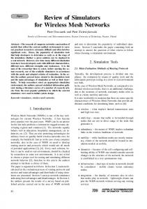
Referring to Figure 1.1, let T = {t} denote a regular partition of the domain Ω into triangular elements. The dual mesh (control volumes) B = {b} of T is constructed by connecting the barycenter and the midpoint of sides of every triangle t ∈ T with straight lines. Let P 1 (T ) denote the space of continuous piecewise linear polynomials associated with T . The usual nodal basis for P 1 (T ) is denoted by {Li }, which satisfies Li (vj ) = δij 4

Figure 1.1: An example control volume mesh. The triangulation T is in solid lines and the control volumes B are in dashed lines. where vj is a vertex in the triangulation. Let P 0 (B) denote the space of discontinuous piecewise constants with respect to B. Define P+0 (T ) = {c ∈ P 0 (T ) : c > 0} to be the space of discontinuous piecewise positive constants with respect to T .

1.5

FEM and CVFE

The similarity of linear finite elements and the box method for Laplacian problems has been discussed [21]. It has been shown that the formulation derived from linear finite elements and the CVFE are the same for incompressible single phase flow problems [18]. The multiphase finite element formulation used in the field of oil reservoir simulation finds the approximations of phase potential and phase saturation in P 1 (T ). The mass-lumping scheme is applied to stabilize the phase saturation values. As a result of mass-lumping, we can consider that the phase saturation solution is sought in P 0 (B). Therefore, a set of control volumes is implied in the FEM. The CVFE method also finds its discretized phase potential in P 1 (T ) and phase saturation in P 0 (B). If the potential-based upstream weighting scheme is applied to the FEM and the CVFE, and both ρ and λ are taken to be the upstream weighted values then the formulations derived from both methods are exactly the same. As a result, the control volumes implied in the FEM are the same as the control volumes B defined in the CVFE. For both methods, we consider both k and φ are in P+0 (T ). The three residual functions for any triangle t ∈ T derived by both methods are i h Fi = − A ρλ up(ij) Tij (ϕj − ϕi ) + ρλ up(ik) Tik (ϕk − ϕi ) (1.11) A ∂(φρi Si ) + (i, j, k = 1, 2, 3 and i 6= j 6= k), 3 ∂t where A is the area of the triangle. Note that the subscript l and the source term 5

in (1.3) are omitted for simplicity. The transmissibility is defined as ∂L ∂L ∂Li ∂Lj ∂Li ∂Lj ∂Li ∂Lj i j + kxy + kyx + kyy Tij = − kxx . ∂x ∂x ∂x ∂y ∂y ∂x ∂y ∂y The potential-based upstream operator is defined by ( i if ϕi > ϕj , up(ij) = j if ϕi < ϕj .

(1.12)

(1.13)

Notice that when the two flux terms of (1.11) are considered separately there is no significant physical meaning associated with either one of them. It is arranged so only to resemble (1.10). A positive transmissibility condition is necessary to guarantee Tij > 0 [16]. Negative transmissibilities are physically unrealistic and also produce unacceptable saturation values.

1.6

The Control Volume Method

In this section, we derive the CVM from a finite element point of view with a focus on the explict expression for local fluid flux. The basic concept of the CVM is to use the fluid potential values on T for flux calculation; the flux so obtained is then used for mass balance on B. Take any triangle t ∈ T as an example; after establishing the flux direction in the triangle, the fluid exchanged between the three control volumes in the triangle can be calculated.

1.6.1

Control volume formulation

The residual function for a control volume bi ∈ B with boundary Γi is obtained by taking the integrated form of (1.1): Z ∂(φρS) i F =0= ∇ · ρv + dx ∂t bi Z Z (1.14) ∂(φρS) dx = ρv · n ˆ ds + ∂t Γi bi Here n ˆ is the unit outward normal on Γi . Note that the subscript l and the source term in (1.3) are omitted for simplicity.

1.6.2

Control volume discretization

During the process of computation, it is difficult to evaluate (1.14) because a control volume is usually distributed accross several triangular elements as shown 6

t3 t2 t4 bi

Γi

t1 t5

Figure 1.2: A control volume with its boundaries across several triangular elements.

=

+

+...

Figure 1.3: Decomposition of a control volume into several subvolumes. in Figure 1.2. A more convenient approach is then to use an element-by-element method to add up the contributions from subvolumes bi,m = bi ∩ tm . Figure 1.3 shows this concept. The residual function for the control volume bi in Figure 1.2 can then be obtained by 5 X Fi = Fmi . (1.15) m=1

The partial residual function by bi,m and is defined as Z i Fm =

Fmi

Γim

represents the part of F i which is contributed

ρv · n ˆ ds +

Z

bi,m

∂(φρS) dx, ∂t

(1.16)

where Γim = Γi ∩ tm .

1.6.3

Formulation of partial residual functions

As shown in Figure 1.4, the partial residual function Fmi of bi,m is derived in this section. The same procedure can be applied to obtain Fmj and Fmk .

7

k ki

bk,m ˆ n

bi,m

jk

c

i

ˆ n

bj,m

ij j

Figure 1.4: Unit outward normals of subvolume bi,m in triangle tm . Equation (1.16) is rewritten for bi,m as Z Z ∂(φρS) i Fm = dx ρv · n ˆ ds + ∂t cij+cki bi,m Z Z Z ∂(φρS) dx = ρv · n ˆ ds + ρv · n ˆ ds + ∂t cij cki bi,m

(1.17)

where n ˆ is the unit outward normal of the corresponding boundary as shown in Figure 1.4. Define the fluxes flowing out of bi,m through cij and cki as Z Z ρv · n ˆ ds and fi,cki = ρv · n ˆ ds, fi,cij = cij

cki

respectively. Also, define the total flux flowing out of bi,m as fi = fi,cij + fi,cki , then equation (1.17) becomes Fmi

= fi +

Z

bi,m

∂(φρS) dx. ∂t

(1.18)

Notice that fi in equation (1.18) represents the flux portion of the partial residual function. The flux across cij is evaluated as Z Z fi,cij = ρv · n ˆ ds = ρ vx î + vy ˆj · nx î + ny ˆj ds cij Zcij (1.19) ρ(vx nx + vy ny ) ds, = cij

where ∂ϕ ∂ϕ + kxy , vx = −λup kxx ∂x ∂y

∂ϕ ∂ϕ vy = −λup kyx + kyy . ∂x ∂y 8

To obtain the unit outward normal n ˆ along a line αβ, a transformation matrix is introduced cos θ − sin θ Tθ = . (1.20) sin θ cos θ

By multipling Tθ to any vector v, a new vector v θ rotated θ degree with respect − → to v is obtained. Let αβ = (xβ − xα , yβ − yα ) represent the vector from node α to node β; then − → αβ (1.21) n ˆ θ = T θ − →

αβ

− → is the unit vector formed by rotating αβ by θ degrees. To find the unit outward normal n ˆ of the control volume bi,m along cij, we let θ = −π/2 then, ← − (yc − yij ) ˆ (xij − xc ) ˆ cij = ← n ˆ = T −π ← i + ← j − − − 2

cij

cij cij

← − where cij = (xc − xij , yc − yij ). Therefore, Z ∂ϕ (yc − yij ) ∂ϕ ρup λup − kxx fi,cij = + kxy

← −

cij

∂x ∂y cij ∂ϕ ∂ϕ (xij − xc ) + kyy ds. − kyx

← −

cij

∂x ∂y

(1.22)

The phase potential in (1.22) is approximated by ϕh ∈ P 1 (T ) and ϕh (x) = Li (x)ϕi + Lj (x)ϕj + Lk (x)ϕk

where ϕi , ϕj , and ϕk are the phase potential values at triangular vertices. Consequentlly, the derivatives of ϕh are constants in t ∈ T ; therefore, (1.22) can be written as h ∂ϕ ∂ϕ + kxy (yc − yij ) fi,cij = ρup λup − kxx ∂x ∂y (1.23) ∂ϕ i ∂ϕ − kyx + kyy (xij − xc ) . ∂x ∂y The flux fi,cki can be derived in the same way as fi,cij and as a result fi is fully defined. Let S be approximated by Sh ∈ P 0 (B) then Sh (bi ) = Si where Si is the saturation value of control volume bi . The partial residual function of bi,m can then be written as ∂(φρi Si ) , (1.24) Fmi = fi + bi,m ∂t

9

k

ki

fcki c

i

fcjk

jk

fcij ij j

Figure 1.5: A schematic representation of the applicable upstream nodes and flux directions. R where bi,m = bi,m dx. Other fluxes can be calculated in the same way and are summarized here. h ∂ϕ ∂ϕ + kxy fi,cij = −fj,cij = ρup λup − kxx (yc − yij ) ∂x ∂y (1.25a) ∂ϕ i ∂ϕ − kyx + kyy (xij − xc ) , ∂x ∂y h ∂ϕ ∂ϕ fj,cjk = −fk,cjk = ρup λup − kxx + kxy (yc − yjk ) ∂x ∂y (1.25b) i ∂ϕ ∂ϕ + kyy (xjk − xc ) , − kyx ∂x ∂y h ∂ϕ ∂ϕ fk,cki = −f1,cki = ρup λup − kxx + kxy (yc − yki ) ∂x ∂y (1.25c) ∂ϕ i ∂ϕ − kyx + kyy (xki − xc ) . ∂x ∂y Note that the first equality in (1.25) states the fact that any flux flowing out of one control volume equals the flux flowing into another control volume through their common boundary within a triangular element. Thus, the CVM is a flux continuous numerical method.

1.6.4

Upstream weighting

The upstream weighted properties in the CVM are determined by the flux-based upstream weighting scheme (unlike the CVFE where the discretized equations are reformulated to resemble the finite difference formulation and a potential-based approach is used). The concept of flux-based upstream weighting in the CVM is better explained by examples. Figure 1.5 shows an example triangle with constant flux across the 10

A fA

ΓAB B fB

Figure 1.6: An illustration of the concept of flux continuity. three control volume boundaries. The upstream properties can then be determined for each flux as follows. 1. For fcij , up = j; 2. for fcjk , up = k; 3. for fcki , up = k. During the programming implementation, the upstream direction is determined by the sign of the flux. Recall the definition of fi ; when fi > 0 the flux is flowing out of the control volume i. Therefore, the flux-based upstream operator up(ij) for the CVM is defined as ( i if fi,cij > 0, (1.26) up(ij) = j if fj,cij > 0. Remark 1.1 For simplicity, the same symbol up(ij) is used for the upstream operator in (1.13) and (1.26). There should be no confusion about which equation to use when up(ij) is encountered.

1.7

Flux continuity

The term flux continuity for a control volume based method is defined as follows. Definition 1.1 A control volume based numerical method is flux continuous if and only if flux is defined on the control volume boundaries, and the flux flowing out of a control volume is exactly the same as the flux flowing into another control volume through their common boundary. This concept is shown in Figure 1.6 where fA is the flux flowing out of control volume A and fB is the flux flowing into control volume B through their common boundary ΓAB . For the numerical method to be flux continuous we require fA + fB = 0.

(1.27)

In the remainder of this section we show that the CVM is flux continuous and prove that the CVFE is not flux continuous. 11

1.7.1

CVM

Equation (1.25) provides expressions for pairs of fluxes entering and leaving control volumes through identified boundaries. Examinzation of this equation shows that the fluxes entering and leaving a boundary add to zero, thus satisfying the definition of flux continuity.

1.7.2

FEM and CVFE

The FEM and CVFE are considered together because they yield the same discretized equations. To prove that these two methods are not flux continuous, a general case is studied to show that the CVFE formulation satisfies Definition 1.1 if and only if the phase potentials at every node are equal. Consequentlly, when there is finite flux, the CVFE is not flux continuous. Theorem 1.1 Consider a triangular element tm ∈ T with arbitrary shape and orientation. The CVFE fluxes between the control volumes {bi , bj , bk } ∈ B in tm are continuous if and only if the phase potential at three triangle vertices are equal, that is ϕi = ϕj = ϕk . Proof 1 For simplicity, this proof is show for the case where kx 0 ∈ P+0 (T ). k= 0 ky As discussed in §1.5, the CVFE formulation was rearranged for upstream implementation. To study the flux continuity property of this method, (1.11) must be returned to its original flux-significant formulation. Starting with the flux portion of (1.11), the flux into and out of bi is separated into x- and y-components. h ∂L ∂Lj ∂Lk i fi = A k x ρλ up(ij) (ϕj − ϕi ) + ρλ up(ik) (ϕk − ϕi ) ∂x ∂x ∂x i ∂Li ∂Lj ∂Lk + ky ρλ up(ij) (ϕj − ϕi ) + ρλ up(ik (ϕk − ϕi ) , ∂y ∂y ∂y

For each component, the fluxes through different straight line boundaries are further separated. Referring to Figure 1.4, since yj − y k yij − yki yij − yc yc − yki ∂Li = = = + , ∂x 2A A A A ∂Li xk − x j xki − xij xki − xc xc − xij = = = + , ∂y 2A A A A

(1.28a) (1.28b)

the total flux can be written as fi = fix,cij + fix,cki + fiy,cij + fiy,cki , 12

(1.29)

which is the summation of the x-direction flux across cij, cki and y-direction flux across cij, cki, respectively. The flux terms are defined by h i ∂Lj ∂Lk (ϕj − ϕi ) + ρλ up(ik) (ϕk − ϕi ) fix,cij = kx (yij − yc ) ρλ up(ij) ∂x ∂x i h ∂Lk ∂Lj (ϕj − ϕi ) + ρλ up(ik) (ϕk − ϕi ) fix,cki = kx (yc − yki ) ρλ up(ij) ∂x ∂x h i ∂Lj ∂Lk fiy,cij = ky (xc − xij ) ρλ up(ij) (ϕj − ϕi ) + ρλ up(ik) (ϕk − ϕi ) ∂y ∂y h i ∂Lj ∂Lk fiy,cki = ky (xki − xc ) ρλ up(ij) (ϕj − ϕi ) + ρλ up(ik) (ϕk − ϕi ) . ∂y ∂y

Similar x- and y-direction fluxes can be derived for bj and bk and are listed here. For bj , (1.30) fj = fjx,cjk + fjx,cij + fjy,cjk + fjy,cij , where h ∂Li fjx,cjk = kx (yjk − yc ) ρλ up(ij) (ϕi − ϕj ) + ∂x h ∂Li (ϕi − ϕj ) + fjx,cij = kx (yc − yij ) ρλ up(ij) ∂x h ∂Li fjy,cjk = ky (xc − xjk ) ρλ up(ij) (ϕi − ϕj ) + ∂y h ∂Li fjy,cij = ky (xij − xc ) ρλ up(ij) (ϕi − ϕj ) + ∂y

For bk ,

i ∂Lk (ϕ − ϕ ) k j up(jk) ∂x i ∂Lk ρλ up(jk) (ϕk − ϕj ) ∂x i ∂Lk ρλ up(jk) (ϕk − ϕj ) ∂y i ∂Lk ρλ up(jk) (ϕk − ϕj ) . ∂y ρλ

fk = fkx,cki + fkx,cjk + fky,cki + fky,cjk ,

(1.31)

where h ∂Li fkx,cki = kx (yki − yc ) ρλ up(ki) (ϕi − ϕk ) + ∂x h ∂Li fkx,cjk = kx (yc − yjk ) ρλ up(ki) (ϕi − ϕk ) + ∂x h ∂Li (ϕi − ϕk ) + fky,cki = ky (xc − xki ) ρλ up(ki) ∂y h ∂Li fky,cjk = ky (xjk − xc ) ρλ up(ki) (ϕi − ϕk ) + ∂y

i ∂Lk (ϕ − ϕ ) j k up(kj) ∂x i ∂Lk ρλ up(kj) (ϕj − ϕk ) ∂x i ∂Lk ρλ up(kj) (ϕj − ϕk ) ∂y i ∂Lk ρλ up(kj) (ϕj − ϕk ) . ∂y

ρλ

For the CVFE formulation to be flux continuous, we require the x- and y-direction fluxes through each interface to satisfy Definition 1.1. Therefore, the CVFE is flux continuous if and only if the following equations are all true. fiu,cij + fju,cij = 0,

(1.32a)

fju,cjk + fku,cjk = 0,

(1.32b)

fku,cki + fiu,cki = 0

where u = {x, y}. 13

(1.32c)

Consider (1.32a). h ∂Li ∂Lj + (ϕj − ϕi ) 0 = kx (yij − yc ) ρλ up(ij) ∂x ∂x i (1.33a) ∂Lk ∂Lk + ρλ up(ik) (ϕk − ϕi ) + ρλ up(jk) (ϕj − ϕk ) ∂x ∂x h ∂Li ∂Lj 0 = ky (xc − xij ) ρλ up(ij) (ϕj − ϕi ) + ∂y ∂y i (1.33b) ∂Lk ∂Lk (ϕk − ϕi ) + ρλ up(jk) (ϕj − ϕk ) + ρλ up(ik) ∂y ∂y

The only possibility for (1.33) to be true for any regular shape and any orientation of triangular element is when ϕk ≥ ϕ i = ϕ j .

(1.34)

The same argument can be applied to (1.32b) and (1.32c), and we have ϕi ≥ ϕ j = ϕ k , ϕj ≥ ϕ i = ϕ k ,

(1.35) (1.36)

respectively. From (1.34), (1.35), and (1.36), we conclude that the CVFE is flux continuous only if ϕi = ϕj = ϕk . On the other hand, if ϕi = ϕj = ϕk then (1.32) is true and the CVFE is flux continuous. Therefore, we have proved that the CVFE is flux continuous if and only if the phase potentials at three vertices are equal. Remark 1.2 The only difference between the CVFE and the CVM is the choice of upstream properties. If (1.32a) is derived using the CVM, all the upstream properties would have been assigned to the values of the same control volume, and for u = x fix,cij + fjx,cij = kx (yij − yc ) ρλ = 0,

h ∂Li ∂Lj ∂Lk ∂Lk + (ϕk − ϕi ) + (ϕj − ϕk ) (ϕj − ϕi ) + up ∂x ∂x ∂x ∂x

since ∂Li /∂x + ∂Lj /∂x + ∂Lk /∂x = 0.

1.8

Mass conservation

The governing equations for oil reservoir simulations are basically mass conservation equations. It is, therefore, very important to verify that the numerical methods employed in solving the equations are both globally and locally mass conservative. 14

It is well known that both the FEM and CVFE are globally mass conservative. The CVM derived in this paper is also globally mass conservative because the solution is obtained by forcing the set of residual functions to be as close to zero as possible. It is widely believed that the FEM is not a locally mass conservative method. On the other hand, the CVFE is considered to be locally mass conservative. However, both the methods yield exactly the same discretized equations. In view of this, we first recall the definition of local mass conservation [22] and examine the CVFE, CVM and FEM methods. Definition 1.2 A control volume based numerical method is locally mass conservative if and only if flux is defined on the control volume interfaces, and the total fluxes flowing into and out of a control volume is exactly balanced by the accumulation term and the source terms. Consider the CVFE and CVM. Both methods solve the approximated solution by forcing every residual function to be zero. Taking a close look at their residual functions, (1.14), it is seen that Definition 1.2 is satisfied for every control volume. Consequentlly, both methods are locally mass conservative. When the local mass conservation property of the FEM is considered on T , the FEM is not conservative. This is because the flux is not defined on the edge of triangles. On the other hand, if the same control volumes, B, as defined in the CVFE are considered for the FEM then the FEM is also locally mass conservative. This is a logical approach because the FEM implies the existance of B as discussed in §1.5.

1.9

Numerical experiments

First, a simple single element example is considered. The effect of different upstream weighting implementation is discussed. The implication of positive transmissibility condition [16] is also considered. The second example considered is a five-spot injection problem. The results from the CVM and the CVFE are compared; the grid orientation effect is studied.

1.9.1

Single triangle example

The term irreducible phase content used in reservoir engineering is discussed first. Due to the nature of porous media, a fluid phase is only mobile when its saturation value is above its irreducible phase content Sir in the porous medium. This property of the porous medium is reflected in the relative permeability function kr (S). The function kr (S) has the following properties ( = 0 if S ≤ Sir , kr (S) > 0 if S > Sir . 15

k −k∇ϕ

k

bk

ki

bk

jk

y i

c

bj ij

jk

ki

c bi

k

i

jk c bi

bj

bi j

bk ki

ij

j

i

bj ij

j

x ϕk > ϕi = ϕj Sk > Si = Sj = Sir

Figure 1.7: Acute, right-angled, and obtuse triangles used in the discussion of the consequences of applying either the potential- or flux-based upstream condition. Therefore, a fluid phase is immobile if S ≤ Sir even when there exists a potential gradient. The positive transmissibility condition for a single triangle is that all angles are equal to or less than π/2 [16]. Consider the acute triangle in Figure 1.7. Relative values of phase potentials and saturations are indicated in the figure. Assume that the permeability tensor is identity; then, the flux direction is pointed in the negative y-direction. The flux flowing out of bj through cij in the y-direction should be zero because Sj = Sir . However, the actual flux calculated by the CVFE is CVFE: fjy,cij = ky (xij − xc ) ρλ

xj − x i (ϕk − ϕj ) 6= 0. k 2A

It is clear that even if the positive transmissibility condition is satisfied, the CVFE still has unrealistic fluxes. In contrast, the same flux in the CVM is ∂ϕ CVM: fjy,cij = ρλ j ky (xij − xc ) = 0 ∂y

because, λj = 0. Consider the right-angled triangle in Figure 1.7. The potential and saturation conditions in Figure 1.7 require the flux through the boundary cjk should be nonzero. This means that the value of Sj should increase. The flux flowing into bj through cjk in y-direction calculated by the CVFE is CVFE: fjy,cjk = ky (xc − xjk ) ρλ

xj − x i (ϕk − ϕj ). k 2A

It is clear that fjy,cij + fjy,cjk = 0 because (xij − xc ) = −(xc − xjk ). As a result, Sj remains unchanged. Thus, once again, it is possible to develop physically incorrect solutions using CVFE. It is for this reason that CVFE is considered a five-point 16

injection well production well diagonal grid

parallel grid

Figure 1.8: Five-spot injection prodcution pattern used as an example calculation problem. stencil method [18] for the right-angled triangles, leading to grid orientation effects. As for the CVM, we have fjy,cij + fjy,cjk < 0 and Sj increases; therefore, a net flux exists in the diagonal direction. Consider the obtuse triangle in Figure 1.7. For the CVFE formulation, as a result of violating the positive transmissibility condition, we have f jy,cij + fjy,cjk > 0, because xij − xjk > 0. The phase saturation Sj is, therefore, reduced to a value less than Sir , which is physically impossible. In the CVM, we have fjy,cij = 0 and fjy,cjk < 0; therefore, the value of Sj increases.

1.9.2

Five-spot injection problem

The test problem for the proposed CVM and the CVFE is a five-spot water injection problem. The arrangement of production and injection wells is shown in Figure 1.9.2. The distance between any two adjacent production wells is 2000 ft. One injection well is placed at the center of a square formed by four surrounding production wells. The wetting and non-wetting phases considered in this problem are water and oil, respectively. Oil and water are produced from production wells, and water is injected through injection wells. Two types of grids are used for testing the grid orientation effects. In the diagonal grid, the production and injection wells are connected through the diagonal of the grid. In the parallel grid, wells are connected through grid lines. These two subdomains within the larger five-spot pattern are shown in Figure 1.9.2. Each subdomain is discretized into 20 by 20 square blocks. Each square block is further divided into two triangles. It should be noted that the parallel grid domain is twice the size of the diagonal grid domain. The water migration patterns are expected to be identical between the injection and production wells in both cases. The oil production rates at different water injection stages are also expected to be the same for the two grid systems. Reservoir rock and fluid properties are listed in Table 1.1. Initially, oil pressure is at 3000 psia and water saturation is 0.20. Because of the symmetric layout of the wells, no flow boundary conditions are used for the two subdomains in consideration. The total fluid rate for both injection and production wells is 40 17

Table 1.1: Rock and fluid properties used in the example problem. Rock Properties kx 200 md ky 200 md φ 0.10=10% Pc 0 So,ir 0.2 Sw,ir 0.2 kro (So − So,ir )3 krw (Sw − Sw,ir )3 Fluid Properties µo 10 cp µw 1 cp P −14.7 ρo ( 89867.7 + 1)ρo,STC 1 ,2 ρw ρw,STC 1 2

STC = stock tank condition P in psia

stock tank barrels per day (STB/day). Since the simulation domain is only a quarter of the five-spot pattern, the fluid rate is further divided by four and a rate of 10 STB/day is used for each well. Consider the solutions of CVM and CVFE on the diagonal grid. Figure 1.9 shows the legend and Figure 1.10 shows the water saturation contours at different injection stages (different times) for these two methods on the diagonal grid. Close to the injection well, water tends to move evenly along the diagonal and grid lines for the CVM. On the contrary, water tends to move along the grid lines for the CVFE. Figure 1.11 shows the water saturation contours at various pore volumes injected for the two solution methods on the parallel grid. For this grid, water migration patterns using the CVM and CVFE are different both around the injection and production wells. Figure 1.12 shows the oil production rate at production wells for the two numerical methods on the two grids. It is evident that the water breakthrough times (the moment at which the fluid at the production well ceases to be pure oil) are different for the two methods. It is also clear that the CVFE solution for breakthrough times and oil rates for the two grid systems are quite different. The CVFE parallel grid solution provides the quickest breakthrough because of water movement predominantly along grid lines. In this case, the CVM solutions for the two grid systems are almost the same, thus, showing very little grid orientation effect.

18

1.10

Conclusions

The potential-based upstream weighting method, commonly used in control volume finite element (CVFE) numerical schemes for the solution of multiphase porous media problems results in solutions which are not flux continuous. A flux-based upstream weighting procedure which provides flux continuous solutions for control volume methods (CVM) is presented in this paper. The CVM is globally and locally mass conservative. The mass-lumping schemes employed in finite element (FEM) numerical methods for the solution of porous media flow problem imply the same set of control volumes as in CVFE. Both the CVFE and the FEM methods are locally and globally mass conservative. The CVM is not restricted by the positive transmissibility condition that limits the shape of the triangular elements used in CVFE. The upstream weighting scheme in CVFE can result in physically unrealistic fluxes even if the positive transmissibility condition is satisfied. The CVFE and the CVM yield different sets of solutions in a simple five-spot injection-production example. In the diagonal and the parallel grid orientations evaluated for this example, the breakthrough times and oil production rates are expected to be the same; these values calculated by the CVM are close while those from the CVFE are different.

19

Sw 0.7 0.65 0.6 0.55 0.5 0.3

Figure 1.9: Legend for water contour plots. CVM CVFE

Figure 1.10: Comparison of the water saturation contours of the diagonal grid problem solved by the CVM (left) and the CVFE (right). From top to bottom are the contours at 0.1, 0.2 and 0.4 domain pore volume of water injected.

20

CVM

CVFE

Figure 1.11: Comparison of the water saturation contours of the parallel grid problem solved by the CVM (left) and the CVFE (right). From top to bottom are the contours at 0.1, 0.2 and 0.4 domain pore volume of water injected. CVM CVM CVFE CVFE

Oil Production Rate [STB/day]

10

Diagonal Parallel Diagonal Parallel

8

6

4

2

0 300

350

400

450

500

550

600

650

700

Time [days]

Figure 1.12: Comparison of the oil production rates for the CVM and the CVFE on the diagonal and the parallel grids. 21

Chapter 2 The Control Volume Finite Element Method 2.1

Synopsis

Reservoir simulation often requires representing complex, irregular domains and complicated fracture networks. The finite difference method is not capable of handling these complex features; finite element method is a good alternative for representing and modeling these systems. The control volume finite element method (CVFE) is closely related to the finite element method (FEM). They both use the same types of interpolation functions for dependent variables. They differ in the way in which fluid flux between control volumes is calculated. In the FEM method, fluid potentials are approximated without the knowledge of fluxes between nodes; however, in the CVFE, fluid flux between nodes is calculated explicitly, and mass balance is formulated according to the flux. The two-dimensional, two-phase CVFE was developed by Yi-kun Yang [23]. Mathematical formulation of CVFE for three-dimension is discussed in this chapter. Following is the outline of the development of CVFE. In section 2.2, the interpolation functions are derived. Based on the concept of control volume, the discretized residual equations for three-dimensional, two-phase system are formulated in section 2.3. The three-dimensional, three-phase formulations are discussed in section 2.4.

2.2

Area Coordinate System and Interpolation Functions

In this section, the lowest order of interpolation function from the Lagrange family–linear interpolation functions–for tetrahedral elements is discussed. The position of any given point x in a tetrahedral element can be uniquely defined by the volumes enclosed with the vertices of the tetrahedron. As shown 22

in Figure 2.1, x is defined by x = (L0 , L1 , L2 ) = (

V0 V1 V2 , , ). V V V

(2.1)

Notice that L0 + L1 + L2 + L3 = 1;

(2.2)

therefore L3 can not be changed independently without disturbing the values of L0 , L1 and L2 . The linear interpolation functions for a given point x in a tetrahedral element are actually its coordinates. The value of h at x ∈ Ωe can be approximated using the values of h at the vertices and the interpolation functions h(x) =

3 X

hi Li (x).

(2.3)

i=0

Notice that hi denotes the value of h at vertex i of the tetrahedron. It can be seen that the value of ∇h needs to be calculated. In the case that Ω ⊂ 0, kr01 = kr0 = kr (S0 ) • for f0,aikj < 0, kr01 = kr1 = kr (S1 ) Repeating the same procedure, the fluxes across bjkh, chki, dgkj, eikj and fgkh can be derived. The six fluxes across the six boundaries are summarized here f0,aikj = −f1,ajki 1 kr01 ρ01 g = 12 B01 µ01 ∂h ∂h ∂h kxx [(y2 − ya )(z3 − za ) − (y3 − ya )(z2 − za )] + kxy + kxz ∂x ∂y ∂z ∂h ∂h ∂h + kyx [(x3 − xa )(z2 − za ) − (x2 − xa )(z3 − za )] + kyy + kyz ∂x ∂y ∂z ∂h ∂h ∂h + kzy + kzz [(x2 − xa )(y3 − ya ) − (x3 − xa )(y2 − ya )] . + kzx ∂x ∂y ∂z (2.38a) f0,bjkh = −f2,bhkj 1 kr02 ρ02 = g 12 B02 µ02 ∂h ∂h ∂h + kxy + kxz [(y3 − yb )(z1 − zb ) − (y1 − yb )(z3 − zb )] kxx ∂x ∂y ∂z ∂h ∂h ∂h + kyy + kyz [(x1 − xb )(z3 − zb ) − (x3 − xb )(z1 − zb )] + kyx ∂x ∂y ∂z ∂h ∂h ∂h + kzy + kzz + kzx [(x3 − xb )(y1 − yb ) − (x1 − xb )(y3 − yb )] . ∂x ∂y ∂z (2.38b) f3,cikh = −f0,chki 1 kr30 ρ30 g = 12 B30 µ30 ∂h ∂h ∂h + kxy + kxz [(y2 − yc )(z1 − zc ) − (y1 − yc )(z2 − zc )] kxx ∂x ∂y ∂z ∂h ∂h ∂h + kyx + kyy + kyz [(x1 − xc )(z2 − zc ) − (x2 − xc )(z1 − zc )] ∂x ∂y ∂z ∂h ∂h ∂h + kzx [(x2 − xc )(y1 − yc ) − (x1 − xc )(y2 − yc )] . + kzy + kzz ∂x ∂y ∂z (2.38c) 32

f1,dgkj = −f2,djkg 1 kr12 ρ12 g = 12 B12 µ12 ∂h ∂h ∂h kxx + kxy + kxz [(y0 − yd )(z3 − zd ) − (y3 − yd )(z0 − zd )] ∂x ∂y ∂z ∂h ∂h ∂h [(x3 − xd )(z0 − zd ) − (x0 − xd )(z3 − zd )] + kyy + kyz + kyx ∂x ∂y ∂z ∂h ∂h ∂h [(x0 − xd a)(y3 − yd ) − (x3 − xd )(y0 − yd )] . + kzx + kzy + kzz ∂x ∂y ∂z (2.38d) f1,egki = −f3,eikg 1 kr13 ρ13 = g 12 B13 µ13 ∂h ∂h ∂h [(y2 − ye )(z0 − ze ) − (y0 − ye )(z2 − ze )] + kxy + kxz kxx ∂x ∂y ∂z ∂h ∂h ∂h + kyx + kyy + kyz [(x0 − xe )(z2 − ze ) − (x2 − xe )(z0 − ze )] ∂x ∂y ∂z ∂h ∂h ∂h + kzy + kzz [(x2 − xe )(y0 − ye ) − (x0 − xe )(y2 − ye )] . + kzx ∂x ∂y ∂z (2.38e) f2,f gkh = −f3,f hkg 1 kr23 ρ23 g = 12 B µ 23 23 ∂h ∂h ∂h kxx + kxy + kxz [(y0 − yf )(z1 − zf ) − (y1 − yf )(z0 − zf )] ∂x ∂y ∂z ∂h ∂h ∂h + kyx + kyy + kyz [(x1 − xf )(z0 − zf ) − (x0 − xf )(z1 − zf )] ∂x ∂y ∂z ∂h ∂h ∂h + kzy + kzz + kzx [(x0 − xf )(y1 − yf ) − (x1 − xf )(y0 − yf )] . ∂x ∂y ∂z (2.38f) Note that the first equalities in equations 2.38 are indicative of the fact that any flux flowing out of one control volume must equal the flux into another control volume through their common control volume boundary. Thus the CVFE is a locally mass(flux) conservative method. The accumulation term is discussed now. The definition of C is defined as Ci = φ BSii . The porosity φ and saturation S are constant within the control volume 33

and B is calculated using the nodal pressure Bi = B(Pi ). As a result, Ci is constant with respect to Vi . Therefore, the accumulation terms in equations 2.23 can be written as Z Z ∂Ci ∂Ci dx = dx ∂t Vi Vi ∂t (2.39) ∂Ci V ∂Ci Vi = . = ∂t ∂t 4 where Vi is the volume for control volume i and V is the total volume of the tetrahedron. To derive the final residual functions for all four control volumes, equations 2.38 and 2.39 are substituted into equations 2.6. After applying implicit Euler time discretization, equation 2.23 becomes V (C n+1 − C0n ), 34t 0 V n+1 n+1 n+1 (C n+1 − C1n ), = f1,ajki + f1,dgkj + f1,eikj + 34t 1 V n+1 n+1 n+1 = f2,bhkj + f2,djkg + f2,f (C n+1 − C2n ), gkh + 34t 2 V n+1 n+1 n+1 = f3,chki + f3,ejki + f3,f (C3n+1 − C3n ). hkg + 34t

n+1 n+1 n+1 F0n+1 = f0,aikj + f0,bjkh + f0,chki +

(2.40a)

F1n+1

(2.40b)

F2n+1 F3n+1

(2.40c) (2.40d)

where the superscripts n+1 and n represent the time levels.

2.4

Three-Dimensional, Three-Phase Simulations

In three-phase simulation, oil, water and gas are present. The solubility of gas in oil as a function of pressure is denoted by the gas-oil ratio (GOR), Rs. Gas emerges from solution when the reservoir pressure falls below the oil/gas bubble point pressure at the given temperature. At this time, gas remains distributed between the oil phase and a free gas phase. Let the subscripts o, w and g represent oil, water and gas components respectively; then the conservation equations for three phases are ∂ 1 −∇ · uo = (2.41) φSo + qo , ∂t Bo ∂ 1 −∇ · uw = (2.42) φSw + qw , ∂t Bw Rs ∂ Sg φ So + φ −∇ · (Rs uo + ug ) = + R s qo + q f g . (2.43) ∂t Bo Bg 34

The flow equations 2.42 and 2.43 for oil and water are the same as the equations for two phases, which are well discussed in the previous sections. In this section only the gas flux term is considered. Z Z F = (Rs uo + ug ) · n ˆ ds = V · n ˆ ds. (2.44) where V = R s uo + u g . Referring to Figure 2.2, the gas flux across aikj is Z f0,aikj = V·n ˆ ds aikj Z ˆ · (nxî + ny ˆj + nz k)ds ˆ = (Vxî + Vy ˆj + Vz k) aikj Z = (Vx nx + Vy ny + Vz nz )ds.

(2.45)

(2.46)

aikj

The volumetric flux is computed by Darcy’s law: ul = −

krl ρl gk∇hl . B l µl

(2.47)

where k is a tensor. The head h is defined as h=

P + z. ρg

(2.48)

Substituting equation 2.47 into equation 2.45, then the flux V is V = −(Rs To ∇ho + Tg ∇hg ). where Tl =

krl ρl gk. B l µl

In three dimensional space, ∂ho ∂ho ∂ho Vx = − Rs Toxx + Toxy + Toxz ∂x ∂y ∂z ∂hg ∂hg ∂hg − Tgxx + Tgxy + Tgxz , ∂x ∂y ∂z ∂ho ∂ho ∂ho + Toyy + Toyz Vy = − Rs Toyx ∂x ∂y ∂z ∂hg ∂hg ∂hg − Tgyx + Tgyy + Tgyz , ∂x ∂y ∂z 35

(2.49)

(2.50)

(2.51a)

(2.51b)

∂ho ∂ho ∂ho + Tozy + Tozz Vz = − Rs Tozx ∂x ∂y ∂z ∂hg ∂hg ∂hg + Tgzy + Tgzz . − Tgzx ∂x ∂y ∂z

(2.51c)

The gas flux across aikj in Figure 2.2 is expanded by substituting equations 2.32 and 2.51 into 2.46 f0,aikj Z =

∂hg ∂ho ∂ho ∂hg ∂hg ∂ho − Rs Toxx − Tgxx + Toxy + Toxz + Tgxy + Tgxz ∂x ∂y ∂z ∂x ∂y ∂z aikj (y3 − ya )(z2 − za ) − (y2 − ya )(z3 − za ) ~ × a2| ~ |a3 ∂ho ∂hg ∂ho ∂ho ∂hg ∂hg − Rs Toyx − Tgyx + Toyy + Toyz + Tgyy + Tgyz ∂x ∂y ∂z ∂x ∂y ∂z (x2 − xa )(z3 − za ) − (x3 − xa )(z2 − za ) ~ × a2| ~ |a3 ∂hg ∂ho ∂ho ∂hg ∂hg ∂ho − Rs Tozx − Tgzx + Tozy + Tozz + Tgzy + Tgzz ∂x ∂y ∂z ∂x ∂y ∂z (x3 − xa )(y2 − ya ) − (x2 − xa )(y3 − ya ) ds. ~ × a2| ~ |a3 (2.52)

~ × a2| ~ with After taking the integrand out and canceling |a3

36

R

aikj

ds, the flux

becomes f0,aikj 1 kro01 ρo01 = Rs g 12 Bo01 µo01 ∂ho ∂ho ∂ho [(y3 − ya )(z2 − za ) − (y2 − ya )(z3 − za )] koxx + koxy + koxz ∂x ∂y ∂z ∂ho ∂ho ∂ho + koyx [(x2 − xa )(z3 − za ) − (x3 − xa )(z2 − za )] + koyy + koyz ∂x ∂y ∂z ∂ho ∂ho ∂ho [(x3 − xa )(y2 − ya ) − (x2 − xa )(y3 − ya )] + kozx + kozy + kozz ∂x ∂y ∂z 1 krg01 ρg01 + g 12 Bg01 µg01 ∂hg ∂hg ∂hg + kgxy + kgxz [(y3 − ya )(z2 − za ) − (y2 − ya )(z3 − za )] kgxx ∂x ∂y ∂z ∂hg ∂hg ∂hg + kgyy + kgyz + kgyx [(x2 − xa )(z3 − za ) − (x3 − xa )(z2 − za )] ∂x ∂y ∂z ∂hg ∂hg ∂ho + kgzx [(x3 − xa )(y2 − ya ) − (x2 − xa )(y3 − ya )] . + kgzy + kgzz ∂x ∂y ∂z (2.53) Repeating the same procedure, the gas fluxes across bjkh, chki, dgkj, eikj and fgkh can be derived.

37

Chapter 3 The Mixed Finite Element Method 3.1

Introduction

The mixed finite element (MFE) method was developed by Raviart and Thomas [24]. To understand this method, consider a second order elliptic model problem on a bounded domain Ω with a Lipshitz continuous boundary Γ: −∇ · u = f u = ∇p p=0

in Ω in Ω on Γ

The variational form of equations (3.1) and (3.2) can be written as Z w (∇ · u + f ) dx = 0 ∀ w ∈ L2 (Ω), Ω Z Z v · u dx + p ∇ · v dx = 0 ∀ v ∈ H(div; Ω), Ω

(3.1) (3.2) (3.3)

(3.4) (3.5)

Ω

respectively. Raviart and Thomas [24] proved that equations (3.4) and (3.5) have a unique solution (u, p) ∈ H(div; Ω) × L2 (Ω). (3.6)

3.1.1

The lowest order Raviart–Thomas space

The zero order Raviart–Thomas space (RT0 ) and triangular elements are used in this research work. The reason for not using higher order Raviart–Thomas space is because of the requirement of upstream weighting, and the reason for using triangular elements is because of the complexity of the geometrical domain.

38

(0, 1) n1 n2

x2

x1

x0 (0, 0)

(1, 0) n0

Figure 3.1: Unit outward normals on triangle’s three edges. RT0 is a special solution space and is normally not well known to people with an engineering mathematical background. The definition of this space is explained, and the properties of this space is discussed. RT0 defines a vector space in multidimensional domains. In triangular elements, RT0 is defined as (3.7) v = (a + c x, b + c y) where the underline denotes that v is a vector, and a, b and c are real numbers. It is more convenient to write v as a combination of three orthogonal (independent) bases in practice. v = v 0 v 0 + v1 v 1 + v2 v 2 (3.8) where v 0 , v 1 , and v 2 are the orthogonal bases, and are defined by equation (3.7). v i = (ai + ci x, bi + ci y). These bases can be found by solving the following equations ( 1 if i = j, (v i · nj ) x = for i, j = 0, 1, 2 j 0 if i 6= j,

(3.9)

(3.10)

where xj is the midpoint of triangle’s side j, and nj is the unit outward normal at xj as shown in Figure 3.1. The three bases for the triangle shown in Figure 3.1 are v 0 = (x, y − 1) √ √ v 1 = ( 2 x, 2 y) v 2 = (x − 1, y).

39

(3.11) (3.12) (3.13)

It can be shown that Z

t

v i · v j dx =

(

2 |t|/3 if i = j, 0 if i 6= j

(3.14)

where t is the triangle in Figure 3.1, and |t| is the area of t.

3.2

Application of the MFEM in reservoir simulation

The mixed finite element method has been applied to miscible flow problem [25] and incompressible two-phase flow problem [26]. A triangle-based mixed finite element - finite volume formulation was developed for compositional reservoir simulation [27]. This formulation uses total flux approximation and IMPES scheme. An expanded mixed finite element method has been developed for accurate and efficient treatment of irregular domains [28]. The expanded method involves a coordinate mapping into one regular computational grid. When the matrix permeability is full-tensor, this formulation has 9-points stencil in two-dimensional space and 19-points stencil in three-dimensional space.

3.3

Multiphase MFE formulation

The extension of the MFE method from the model elliptic problem, equations (3.1) to (3.3), to a time-dependent, multiphase flow problem is not a simple matter. The extension is discussed here.

3.3.1

Multiphase flow equations

The governing equation for multiphase subsurface flow problems is the phase volumetric balance equation: ∂ φS + q. (3.15) −∇ · u = ∂t B The phase subscripts for each variable are omitted for brevity. The volumetric flux is computed by the multiphase Darcy’s law: u=−

kr ρ g k∇h Bµ

(3.16)

where the double underlines indicate that k is a tensor. The head is defined as h=

P + z. ρg 40

(3.17)

The relative permeability kr in equation (3.16) could degenerate to zero causing u = 0 even though the head gradient is not zero, therefore u cannot be used as the flux in the MFEM context. Instead, the modified head gradient is used f = −k∇h,

(3.18)

and the multiphase Darcy’s law becomes u=

kr ρ gf Bµ

(3.19)

The variational form of (3.15) and (3.18) are Z Z Z ∂ φS dx + wq dx = 0, w∇ · u dx + w ∂t B Ω Ω Ω Z Z v · f dx = − v · k · ∇h dx, Ω

(3.20) (3.21)

Ω

respectively.

3.3.2

Discretization

Consider solving the multiphase equations on a polygonal domain Ω, and the domain is partitioned (meshed) into a set of regular triangles T . The choice of w in equation (3.20) for a triangle T in T is ( 1 if x ∈ T , w(x) = (3.22) 0 if x ∈ / T. Substituting w(x) into equation (3.20), the variational balance equation becomes an integral equation Z Z Z ∂ φS ∇ · u dx + dx + q dx = 0. (3.23) B T ∂t T T The choice of v in equation (3.21) for t is ( v i (x) if x ∈ T , v i (x) = 0 if x ∈ /T

for i = 0, 1, 2.

(3.24)

After substituting equation (3.24) into equation (3.21), the variational flux equation becomes Z Z (3.25) v i · f dx = − v i · k · ∇h dx, for j = 0, 1, 2. T

T

41

There will be a volumetric balance equation and three volumetric flux equations for each triangle in T . The solution space for h and S is piecewise constant, and the space for f is RT0 . Consequently, the integral equation (3.23) can be simplified to 2 X |T | φS φS − + |T | q = 0 (3.26) (u · n) x li + i ∆t B B i=0

where li is the length of side i, |T | is the area of T . Replacing f on the left of equation (3.25) with equation (3.8), the equation is simplified to Z 2 |T | v i · f dx = fi . (3.27) 3 T Applying integration by parts to the right of equation (3.25), Z Z Z h ∇·q i dx − ∇·(q i h) dx − v i · k ∇h · dx = T T Z ZT h ∇·q i dx − = h q i · n ds T

∂T

= h |T | ∇·q i − where

2 X j=0

(3.28)

hj (q j · nj ) x lj j

(3.29)

qi = vi · k

and hj is the phase head on T ’s side j. Equate equations (3.27) and (3.28). 2

Therefore,

X 2 |T | fi = h |T | ∇·q i − hj (q j · nj ) x lj . j 3 j=0

(3.30)

2

3 3 X fi = h∇·q i − hj (q j · nj ) x lj . j 2 2 |T | j=0

(3.31)

The first term of equation (3.26) can be simplified to

2 2 X X kr ρ u x · ni li = g f x · n i li i i Bµ i=0 i=0

=

2 X kr ρ i=0

Bµ

g f i li

The final volume balance equation for T is " n # 2 n+1 X φS kr ρ |T | φS − g f i li + + |T | q = 0 Bµ ∆t B B i=0

where fi is defined by equation (3.31).

42

(3.32)

(3.33)

3.3.3

Discretized multiphase flow equations

The discretized multiphase flow equations are derived in this section. The volumetric balance equation (3.15) is rewritten here for convenience. ∂ φS −∇ · u = + q. (3.34) ∂t B Let the subscripts o, w and g represent oil, water and gas phases, respectively, then the three-phase volumetric balance equations are ∂ φSo + qo , (3.35) −∇·uo = ∂t Bo ∂ φSw −∇·uw = + qw , (3.36) ∂t Bw ∂ φSg φSo −∇·ug − Rs ∇·uo = + q g + R s qo . (3.37) + Rs ∂t Bg Bo Referring to equation (3.33), the discretized three-phase equations for triangle T can be written as " n+1 n # 2 X kro ρo |T | φSo φSo g fio li + + |T | qo , (3.38) 0= − B o µo ∆t Bo Bo i=0 " n+1 n # 2 X krw ρw φSw |T | φSw g fiw li + − 0= + |T | qw , (3.39) B w µw ∆t Bw Bw i=0 " n+1 n # 2 X φSg φSg krg ρg |T | − 0= g fig li + + |T | qg B g µg ∆t Bg Bg i=0 " (3.40) n+1 n # 2 X |T | φSo φSo kro ρo + |T | Rs qo . g fio li + − Rs Rs + Rs B o µo ∆t Bo Bo i=0 The modified head gradients for each phase on each side of T are 2

3 3 X fio = ho ∇·q i − hjo (q j · nj ) x lj , j 2 2 |T | j=0

2 3 3 X fiw = hw ∇·q i − hjw (q j · nj ) x lj , j 2 2 |T | j=0

(3.41) (3.42)

2

3 X 3 hjg (q j · nj ) x lj . fig = hg ∇·q i − j 2 2 |T | j=0 43

(3.43)

3.3.4

Flux continuity

Equations (3.41) to (3.43) are defined as the fluxes flowing out of a triangle through side i. Flux continuity between neighbor triangles was not imposed in those equations. Three additional balance equations for each edge are necessary to enforce flux continuity. Consider two triangles T1 and T2 sharing a common edge γ. The flux continuity is ensured by solving the following equations T1 T2 0 = fγo + fγo

0= 0=

T1 fγw T1 fγg

T2 + fγw T2 + fγg .

(3.44) (3.45) (3.46)

The superscript indicates which triangle the flux is originated from. The first subscript indicates the edge these two fluxes are flowing through. The second subscript indicates phase.

44

Chapter 4 Verification A synthesized oil reservoir was used to compare the UFES (Utah Finite Element Simulator) and Eclipse (a commercial oil reservoir simulator). The reservoir measures 1000 feet in the ease-west direction, 500 feet in the north-south direction, and is 50 feet thick (Figure 4.1). Two horizontal wells were modeled. The horizontal production well was placed in the top layer on the north side and the horizontal injection well was placed in the bottom layer on the south side. Primary oil production was begun at a production liquid rate of 1000 stb/day and was continued for 90 days. At 90 days, the production liquid rate is reduced to 600 stb/day and water injection was started. At 3600 days, the injection and production were stopped. This scenario was constructed to capture the essentials of the three-phase flow processes; oil and gas flow, gas evolution, gas pressurization, and oil and water flow. Two meshes were used to study the production process. The first mesh has only one layer, and therefore gravitational effect is inconsequential. The second mesh has two layers and gas segregation and water under-ride due to gravity are expected. These two case studies are described in the following sections.

4.1

One-layer case study

The simulation domain is discretized into 40×20×1 blocks for Eclipse. As for UFES, the domain is discretized into 1330 tetrahedrals all expanded over entire thickness. Plots of cumulative oil production versus time are presented in Figures 4.3 and 4.4. Figures 4.5 and 4.6 are the oil production rate curves. Water cut data are shown in Figures 4.7 and 4.8. Gas to oil ratios are shown in Figures 4.9 and 4.10.

4.2

Two-layer case study

The domain of interest was divided into two layers. The grid used for Eclipse is 20×10×2 blocks. The grid for the UFES has two layers and each layer is further 45

discretized into 300 tetrahedrals. Figures 4.12 and 4.13 present the cumulative oil production curve for this case study. The oil production rate plots are shown in Figures 4.14 and 4.15. Water cut plots are shown in Figures 4.16 and 4.17. Gas to oil ratios are presented in Figures 4.18 and 4.19.

4.3

Summary

It should be emphasized that these are fundamentally very different simulators. The finite-element simulator has been developed primarily for representing complex domains including faulted and fractured systems. It is also appropriate for modeling complex well systems (multilaterals, fish-bones, etc.) The well models for UFES were developed at the University of Utah. Considering the fundamentally different discretization, and different well models, the match between the three-phase UFES and Eclipse is excellent. A new three-dimensional, threephase, finite-element simulator is available for use. We would like to study the application of the model to complex geologic systems.

46

Figure 4.1: The domain measures 1000 ft in the x-direction, 500 ft in the ydirection and 50 ft in the z-direction. The horizontal production well is represented by the the orange line and the horizontal injection well is represented by the blue line. Wells are placed at the center of the domain along the x-direction, and each well measures 800 ft in length.

Figure 4.2: The mesh used for the one-layer case study for the UFES.

47

Cumulative Oil (fraction OOIP)

0.5 0.45 0.4 0.35 0.3 0.25 0.2 0.15 0.1 UFES Eclipse

0.05 0 0

500

1000

1500

2000

2500

3000

3500

Time (days)

Figure 4.3: Cumulative oil production for the one-layer case study.


0.45 0.4 0.35 0.3 0.25 0.2 0.15 0.1 UFES Eclipse

0.05 0 0

200

400

600

800

1000

Time (days)

Figure 4.4: A more detailed cumulative oil production plot for the one-layer case study (between zero and 1000 days).

48

1000 UFES Eclipse

900 Oil rate (stb/day)

800 700 600 500 400 300 200 100 0 0

200

400

600

800

1000

Time (days)

Figure 4.5: Oil production rate for the one-layer case study.

600

Oil rate (stb/day)

595 590 585 580 575 570

UFES Eclipse

565 100

120

140

160

180

200

Time (days)

Figure 4.6: A more detailed oil production plot for the one-layer case study (between 91 and 200 days). Notice that the y-axis has a higher resolution.

49

1 0.9 0.8 Water cut

0.7 0.6 0.5 0.4 0.3 0.2 UFES Eclipse

0.1 0 0

200

400

600

800

1000

1200

1400

Time (days)

Figure 4.7: Water cut for the one-layer case study.

0.06 0.05

UFES Eclipse

Water cut

0.04 0.03 0.02 0.01 0 100

120

140

160

180

200

Time (days)

Figure 4.8: Water cut data between 91 and 200 days for the one-layer case study. Notice that the y-axis has a higher resolution

50

16 UFES Eclipse

14 GOR (Mscf/stb)

12 10 8 6 4 2 0 0

50

100

150

200

Time (days)

Figure 4.9: Gas oil ratio for the one-layer case study.

16 UFES Eclipse

14 GOR (Mscf/stb)

12 10 8 6 4 2 0 95

100

105

110

115

120

125

130

Time (days)

Figure 4.10: Gas oil ratio between 91 and 130 days for the one-layer case study.

51

Figure 4.11: The mesh used for the two-layer case study for the UFES.

52


0.6 0.5 0.4 0.3 0.2 0.1

UFES Eclipse

0 0

500

1000

1500

2000

2500

3000

3500

Time (days)

Figure 4.12: Cumulative oil production for the two-layer case study.


0.5 0.45 0.4 0.35 0.3 0.25 0.2 0.15 0.1 UFES Eclipse

0.05 0 0

200

400

600

800

1000

Time (days)

Figure 4.13: Cumulative oil production curve between 0 and 1000 days for the two-layer case study.

53

1000 UFES Eclipse


800 700 600 500 400 300 200 100 0 0

200

400

600

800

1000

Time (days)

Figure 4.14: Oil production rate for the two-layer case study.

600

Oil rate (stb/day)

590 580 570 560 550

UFES Eclipse

540 100

120

140

160

180

200

Time (days)

Figure 4.15: Oil production rate between 91 and 200 days for the two-layer case study.

54

1 0.9 0.8 Water cut

0.7 0.6 0.5 0.4 0.3 0.2 UFES Eclipse

0.1 0 0

200

400

600

800

1000

1200

1400

Time (days)

Figure 4.16: Water cut for the two-layer case study.

0.09 0.08

UFES Eclipse

0.07 Water cut

0.06 0.05 0.04 0.03 0.02 0.01 0 100

120

140

160

180

200

Time (days)

Figure 4.17: Water cut between 91 and 200 days for the two-layer case study.

55

18 UFES Eclipse

16

GOR (Mscf/stb)

14 12 10 8 6 4 2 0 0

50

100

150

200

Time (days)

Figure 4.18: Gas oil ratio for the two-layer case study.

18 UFES Eclipse

16

GOR (Mscf/stb)

14 12 10 8 6 4 2 0 95

100

105

110

115

120

125

130

Time (days)

Figure 4.19: Gas oil ratio between 91 and 130 days for the two-layer case study.

56


0.6 0.5 0.4 0.3 0.2 0.1

UFES Eclipse

0 0

500

1000

1500

2000

2500

3000

3500

Time (days)

Figure 4.20: Cumulative oil production for the two-layer case study.


0.5 0.45 0.4 0.35 0.3 0.25 0.2 0.15 0.1 UFES Eclipse

0.05 0 0

200

400

600

800

1000

Time (days)

Figure 4.21: Cumulative oil production curve between 0 and 1000 days for the two-layer case study.

57

1000 UFES Eclipse


800 700 600 500 400 300 200 100 0 0

200

400

600

800

1000

Time (days)

Figure 4.22: Oil production rate for the two-layer case study.

600 599.5 Oil rate (stb/day)

599 598.5 598 597.5 597 596.5 UFES Eclipse

596 595.5 100

120

140

160

180

200

Time (days)

Figure 4.23: Oil production rate between 91 and 200 days for the two-layer case study.

58

1 0.9 0.8 Water cut

0.7 0.6 0.5 0.4 0.3 0.2 UFES Eclipse

0.1 0 0

200

400

600

800

1000

1200

1400

Time (days)

Figure 4.24: Water cut for the two-layer case study.

0.007 UFES Eclipse

0.006

Water cut

0.005 0.004 0.003 0.002 0.001 0 100

120

140

160

180

200

Time (days)

Figure 4.25: Water cut between 91 and 200 days for the two-layer case study.

59

18 UFES Eclipse

16

GOR (Mscf/stb)

14 12 10 8 6 4 2 0 0

50

100

150

200

Time (days)

Figure 4.26: Gas oil ratio for the two-layer case study.

18 UFES Eclipse

16

GOR (Mscf/stb)

14 12 10 8 6 4 2 0 95

100

105

110

115

120

125

130

Time (days)

Figure 4.27: Gas oil ratio between 91 and 130 days for the two-layer case study.

60

Chapter 5 Fractured Reservoir Simulation Naturally fractured oil reservoirs have quite different recovery characteristics compared to non-fractured reservoirs and therein consider the influence of fractures on fluid flow when production strategy is being planed is important. There are currently four different fracture models being used in reservoir simulations: single continuum, dual porosity, dual permeability and discrete-fracture model. A discussion and comparison of these four models can be found in Kim [11]. In current research work, the focus is on the continuation of the discrete-fracture model development. One version of a discrete-fracture model has been implemented by Kim [11] using the finite element method. The same set of governing equations are used for the fluid flow in matrix and in fracture. The final global stiffness matrix is obtained by superimposing the contribution from matrix and fracture. Validation of this model with single continuum model on a fine grid was attempted. Influence of different capillary pressures between fractures and matrix was studied. However, the superimposition was not explained in terms of the underlying physical implication. A new version of a discrete-fracture model is developed in this research work. With the concept of control volumes and explicit calculation of fluxes, the discretefracture model can now be explained in a physically meaningful way. A brief introduction to reservoir fractures is first presented in section 5.1. This is followed by the implementation of discrete-fracture model using the control volume method developed in Chapter 1. Simulations of a fractured offshore oil field are discussed.

5.1

Reservoir Rock Fractures

The formation, classification and evaluation of fractures are ongoing research topics themselves. Therefore, only a short introduction to these subjects are provided here for the completeness of fracture simulation. A reservoir fracture is a macroscopic planar discontinuity in which a loss of cohesion of reservoir rock has taken place [29, 30]. A fracture can, therfore, be 61

considered as a rupture in reservoir rocks. Two of the most common types of fractures are faults and joints. A fault is a fracture along which one side has moved relative to the other [31]. A fracture is regarded as a joint when there is no noticeable displacement along the fracture [29]. Two dimensional representations of a fault and joints are shown in Figure 5.1 and Figure 5.2, respectively. Two common causes of fractures are overburden pressure and tectonic forces. Figure 5.3 shows a fracture created by overbuden prssure and Figure 5.4 shows a pair of conjugated fractures created by tectonic forces. Direct evaluation of fractures includes outcrop observation in the field and core examination in the laboratory [29]. Fracture opening (fracture width), fractrue filling and fracture orientation can be measured during the direct evaluation process. Indirect methods include well logs and seismic data. There are many well logging methods for the evaluation of fractures, for example, induction logs, the combination of sonic, neutron and density logs, gamma ray and borehole televiewer [30].

5.2

Fracture Information from the Field

Before the discussion of fractured reservoir simulation, it is necessary to understand what types of fracture information are available and are given to simulator developers. For simplicity, consider two-dimensional applications. The fracture information of an oil field given by geologists or reservoir engineers are in terms of straignt line segments. The permeability of each fracture is given or estimated from its width. It is not uncommon that the width of fractures are never known. An example data set of a fractured domain Ω is given as follows. The domain with fractures is shown in Figure 5.5. The matrix permeability tensor is given as a function of the location, that is k m = k m (x)

(5.1)

where m stands for rock matrix or simply matrix and x ∈ Ω. Fracture properties are given in Table 5.1. The location and orientation of each fracture is defined fault

Figure 5.1: Cross-section view of a fault. 62

Figure 5.2: Areal view of some joints.

pressure

joint

Figure 5.3: Cross-section view of the formation of a joint caused by overburden pressure.

60◦ tectonic force

tectonic force

Figure 5.4: The formation of a pair of conjugated fractures due to tectonic force.

63

Table 5.1: Fracture properties available from oil field. Fracture No. Start End Permeability width 1 f1 (xs1 , y1s ) (xe1 , y1e ) k1 w1 s e s e f2 (x2 , y2 ) (x2 , y2 ) k2 w2 .. .. .. .. .. . . . . . 1

The width of fractures is not always available.

by its starting and ending points. Fracture permeability k f is given as a scalar which represents the permeability along the fracture line. The width of fractures is sometimes but not always available as shown in the last column of Table 5.1.

5.3

Single-Porosity Model

When the width information of fractures is available, the most straightforward and accurate approach to fracture simulation is the single porosity model. In this model, fractures are represented by very tiny or very thin two-dimensional elements. Consider a square domain with one fracture as shown in Figure 5.6. To put the width of fractures into consideration, the line is replaced by a rectangle and is shown is Figure 5.7. It important to note that the width and the length of the fracture in Figure 5.7 are not in proportion; the width has been enlarged in order to be visible. In general the ratio of length to width of fractues is in the range of four to six orders. The triangular mesh of this single fracture domain is shown in Figure 5.8. It is clear that a trimendous amount of triangles is required by the single-porosity model even for a single, disproportional fracture. Consequentlly, the single-porosity model will need a lot more elements for a real fracture (a fracture that is in correct proportion) than the disproportional fracture.

5.4

Discrete-Fracture Model

In view of the limited fracture information that is available and the difficulty (requires too many elements) involved in the single porosity model, it is natural to consider the use of line elements to approximate fractures in two-dimensional space. Consider the same square domain with one fracture as discussed in section 5.3. Without the introduction of fracture width, the domain is directly triangulated and the result is shown in Figure 5.9. Comparing Figure 5.8 with Figure 5.9, the number of triangular elements required by the single-porosity for a single disproportional fracture is about five times of that required by the discrete-fracture model. When the number of fracture increases and real fracture geometry is used 64

in the single-porosity model, the single-porosity approach becomes impractical because of the amount of nodes and elements involved.

5.5

Case Studies

65

Ω

fracture rock matrix

Figure 5.5: A fractured domain Ω.

Figure 5.6: The original fractured domain.

66

Figure 5.7: The fractured domain after the fracture is replaced by a rectangle; the width of the fracture has been enlarged for visibility.

Figure 5.8: Triangular mesh of the domain using the single-porosity model; there are 415 nodes and 780 triangles in this particular mesh.

67

Figure 5.9: Triangular mesh of the domain using the discrete-fracture model; there are 97 nodes and 160 triangles in this particular mesh.

Matrix k = 5md, φ = 39% k = 8md, φ = 45% Fracture k = 500, 000md k = 50, 000md k = 10, 000md

Figure 5.10: The fractured domain. Different matrix and fracture properties are shown in the legend.

68

Flowing Boundary No-Flow Boundary

Outer Domain

Figure 5.11: The incorporation of the outer domain to simulate the three flowing boundaies.

Figure 5.12: The placement of injection and production wells for Case I; the blue and red lines are the horizontal injection and production wells, respectively.

69

Figure 5.13: The placement of injection and production wells for Case II; the blue and red lines are the horizontal injection and production wells, respectively.

70

Figure 5.14: The placement of injection and production wells for Case III; the blue and red lines are the horizontal injection and production wells, respectively.

Figure 5.15: The placement of injection and production wells for Case IV; the blue and red lines are the horizontal injection and production wells, respectively.

71

Figure 5.16: Water saturation distribution of Case I at 1000 days.

Figure 5.17: Water saturation distribution of Case II at 1000 days.

72

Figure 5.18: Water saturation distribution of Case III at 1000 days.

Figure 5.19: Water saturation distribution of Case IV at 1000 days.

73



74



75



76



77

Cumulative Oil Production (fraction OOIP)

0.6 Case Case Case Case

0.5

I II III IV

0.4

0.3

0.2

0.1

0 0

2000

4000

6000

8000

10000

Time [days]

Figure 5.28: Cumulative oil production versus time for the four case studies.

78

Chapter 6 Examples 6.1

Example 1

In this first example, a complicated two-dimensional domain with several intersecting fractures is simulated. The domain is shown in Figure 6.1. It is difficult to simulate this domain with finite difference representation. In fractured/faulted systems like these, matrix and fracture capillary pressure relationships are critical in establishing recovery patterns. Two different waterflood studies were carried out in this system. • In the first study, the rock matrix capillary pressure was negative (indicative of an oil-wet rock) while the capillary pressure in the fractures was zero. • In the second, the rock matrix capillary pressure was positive (indicative of a water-wet system) while the capillary pressure in the fractures was zero. The water saturations in the domain with negative capillary pressure are shown in Figure 6.2. It is clear that the negative capillary pressure inhibits imbibition, water does not effectively enter the rock matrix from the fractures and oil recovery is poor. The water saturations in the domain with positive capillary pressure in the rock matrix is shown in Figure 6.3. Water floods the matrix efficiently, showing large, invaded blue zones, and recovery is excellent. The simulator makes these types of fundamental studies possible.

6.2

Example 2

In this example, another complex domain, shown in Figure 6.4 is simulated. In a number fields, there are two dominant fracture directions. In this example, both these sets of fractures are shown by white lines. Use of deviating horizontal wells, sometime drilled from the same platform is fairly common, and this field development strategy is simulated. Combinations of these horizontal wells, intersecting fractures and complex boundaries are very difficult, if not impossible to represent 79

Figure 6.1: Plan view of a domain with intersecting fractures is shown. Water injectors are in blue and producers are shown in red.

Figure 6.2: Water saturations as a result of a waterflood in a system with negative rock matrix capillary pressure and zero fracture capillary pressure 80

Figure 6.3: Water saturations as a result of a waterflood in a system with positive rock matrix capillary pressure and zero fracture capillary pressure using existing simulators. Waterflood at early time is shown in Figure 6.5 and at a later time in Figure 6.6. The finite element simulators make it possible to study practical reservoir development in complex fields with fractures/faults and horizontal wells.

6.3

Example 3

Since the success of the waterflood in the Monument Butte Unit, through a U.S. DOE sponsored project with Lomax, Inc. and the University of Utah, over 2000 wells have been drilled in the Greater Monument Butte belt. The target reservoirs are in Greenriver formation. A typical unit consists of wells drilled on a 40-acre spacing. All the wells are hydraulically fracture and are produced for a period ranging from six months to two years. Subsequently, the unit is operated as a five spot waterflood. There can be significant variation in the orientations and lengths of hydraulic fractures; however, in most units the fractures display a dominant direction. The fracture half lengths are of the order of 200 feet. One section, consisting of 16 hydraulically fractured wells is shown in Figure 6.7. The fracture orientation is varied slightly (10-20 degrees) over the dominant northwest-southeast direction and fracture half lengths are varied around 200 feet. This particular simulation had 10,000 elements. The waterflood performance at early and late times is shown in figures 6.8 and 6.9. Simulating these hydraulic fractures with different orientations is very difficult using a structured mesh. The finite element simula81

Figure 6.4: Complex domain with two sets of intersecting fractures (white lines), deviating horizontal injectors (blue lines) and horizontal producers (red lines) is shown.

Figure 6.5: Waterflood at an early time in the domain shown in Figure 6.4 is presented.

82

Figure 6.6: Waterflood at a late time in the domain shown in Figure 6.4 is presented. tors can thus be used to evaluate the effectiveness of hydraulic fracturing, examine early breakthrough phenomena and plan other field management activities.

83

Figure 6.7: A common waterflood unit in the Greater Monument Butte field. The well spacing is 40 acres. All the wells are hydraulically fractured. Slightly different fracture orientations and fracture half lengths of 200 feet area are assumed

Figure 6.8: Waterflood at an early time in the domain shown in Figure 6.7 is presented.

84

Figure 6.9: Waterflood at a a late time in the domain shown in Figure 6.7 is presented.

85

Chapter 7 Example of Three-Dimensional Simulation The three-dimensional simulation was performed by constructing the three-dimensional extension of the two-dimensional domain examined in Example 1 of Chapter 5. The domain was irregular with the total dimensions in the x and in the y directions being about 600 feet. The thickness of the domain was 50 feet. Four intersecting fractures were placed in the domain. These were not all orthogonal the dip angles varied between 70 and 90 degrees. Tetrahedral mesh was created with this system. The domain and the mesh are shown in figures 7.1 and 7.2. A study similar to the one reported for the two-dimensional domain with positive and negative capillary pressures was conducted. The first set of pictures are with negative capillary pressures in the rock matrix. The injection and production rates were 80 barrels per day. The three-dimensional plot of water saturations in the system after 181 days of continuous injection is shown in Figure 7.3. More useful information is obtained when cross-sections within the threedimensional domain are observed. Four Y-Z sections at different x values are shown in Figure7.4. The impact of fractures and the gravity-driven water flow are clearly captured in this figure. The effect of gravity on the water flood can be observed by studying the X-Y sections at different z values. Two such cross sections are shown in figures 7.5 and 7.6. The first cross section in Figure 7.5 is at a z value of 10 feet and the second cross section in Figure 7.6 is at a z value of 40 feet. As expected, the water saturations are uniformly high in the cross section at z equal to 40 feet. These figures also illustrate the fact that imbibition is poor, leading to poor rock matrix sweep. At later times, basically the same trends are observed. Figure 7.7 shows Y-Z cross sections of water saturations after 1003 days of injection and figure 7.8 shows the plan view (X-Y cross section) at the same time. The picture is different when positive capillary pressure values are used for the rock matrix. The three-dimensional view of water saturations after 181 days of injection is shown in figure 7.9. The Y-Z cross sections at the same x values as 86

Figure 7.1: The three-dimensional domain showing the fractures and the tetrahedral mesh

Figure 7.2: Another view of the three-dimensional domain with fractures and the mesh created 87

Figure 7.3: Water saturations in the three-dimensional domain with fractures after 181 days of injection

Figure 7.4: Water saturations at 181 days. Y-Z cross-sections at x values of 174, 380, 488 and 593 feet are shown. 88

Figure 7.5: A plan view (X-Y section) at z=10 feet. Water saturations are after 181 days of injection are shown.

Figure 7.6: A plan view (X-Y section) at z=40 feet. Water saturations after 181 days of injection are shown. 89

Figure 7.7: Water saturations at 1003 days. Y-Z cross-sections at x values of 174, 380, 488 and 593 feet are shown.

Figure 7.8: A plan view (X-Y section) at z=25 feet. Water saturations are after 1003 days of injection are shown. 90

Figure 7.9: Water saturations in the three-dimensional domain with fractures after 181 days of injection; capillary pressures in the rock matrix are positive before are shown in figure 7.10. The effectiveness of the sweep due to imbibition is best illustrated with the plan view of water saturation at z equal of 25 feet after 1003 days of injection (shown in figure 7.11.

91

Figure 7.10: Water saturations for positive capillary pressure in the rock matrix at 181 days. Y-Z cross-sections at x values of 174, 380, 488 and 593 feet are shown.

Figure 7.11: A plan view (X-Y section) at z=25 feet. Water saturations are after 1003 days of injection and the rock matrix capillary pressure is positive 92

Chapter 8 OPTIMIZATION TECHNIQUE AND APPLICATIONS The first part of this chapter outlines the basics of optimization and a general overview of some of the techniques best suited to solve nonlinear optimization problems. In the second part this chapter, the algorithm used for optimization is outlined. The third part demonstrates the application of the algorithm to reservoir examples.

8.1

Description of the Optimization Problem

Optimization is the act of obtaining the best result under given circumstances using efficient quantitative methods. It is important to use established mathematical techniques rather than implement ad hoc procedures to perform optimization. A typical optimization problem is described by a system or process and a measure or criterion that is used to judge the performance of the system, subject to the imposed constraints. The system or the model as it is sometimes called is described by a set of variables known as the states. The entire process is driven by a set of inputs commonly known as control variables. Mathematically, an optimization problem can be written as, Minimize (or Maximize): J(u) Subject to: g(x) = 0 xl ≤ xi ≤ xu i = 1, 2, . . . , n ul ≤ uj ≤ uu j = 1, 2, . . . , m

(8.1) (8.2) (8.3) (8.4)

The optimization problem is described by the nature of the cost function (performance criterion), J(u) in Equation (8.1) and the process defined by Equation (8.2). The state variables of the system are denoted by x and u represents the set of control variables. If the cost function and the process are both linear, the problem is termed as a linear problem. If any one of the function or the system 93

or both are nonlinear, the optimization problem is a nonlinear one. Optimization in reservoir simulation is an example of nonlinear optimization where the state variables are computed by solving nonlinear equations. The reservoir model is dynamic in nature which makes this a dynamic optimization problem. The cost function, even a simple profit function in reservoir engineering, as described later in this chapter, is nonlinear in nature.

8.2

Overview of Nonlinear Optimization Techniques and Applications

Several researchers have successfully implemented formal optimization methods to solve various reservoir engineering problems. This section describes some of the work done in this area of dynamic optimization with reasonable mathematical explanations wherever possible. Many of these methods were considered before deciding on the method used in this work.

8.2.1

Optimal Control Theory

The goal of an optimal control problem is to determine a control policy or a strategy that will maximize or minimize a performance criterion or an objective functional subject to constraints that describe the dynamics of the system. The fundamental theories of this problem are the calculus of variations and Pontryagin’s Maximum Principle. The calculus of variations approach is based on the fundamental theorem of variational calculus [32]. The theorem is applied to problems with no constraints on states and controls. The theorem is coupled with Pontryagin’s Maximum Principle [33] to allow constraints on state and control variables. Ramirez et al. [34] have presented the theory of optimal control of distributedparameter systems where they applied the theory of calculus of variations coupled with Pontryagin’s minimum principle to determine the best surfactant injection policy for tertiary recovery of oil. Fathi and Ramirez [35] applied this theory to maximize the cost of oil recovery while minimizing the cost of surfactant injected. The amount of chemical injected was used as the control variable. The control was updated using a steepest-descent gradient method. This work was extended to determine optimal operating strategies for steamflooding [36] and carbon dioxide miscible-flooding [37] enhanced oil recovery processes processes. Sudaryanto and Yorstos [38] addressed the issue of control of displacement fronts of fluids flowing in porous media. They used optimal control theory to control the injection rates at different point sources. Brouwer and Jansen [39] applied the optimal control theory to optimize the valve settings in smart wells for waterflooding of heterogeneous reservoirs. A gradient based control technique was used to solve the problem. Maximization of the Net Present Value (NPV) was identified as the objective of the problem. 94

8.2.2

Dynamic Programming and its Variations

The dynamic programming (DP) method is a stage-wise procedure which enables one to construct the optimal solution to a multistage decision problem. This technique was developed by Bellman [40] in mid-twentieth century. The technique decomposes a multistage decision problem as a sequence of single-stage decision problems. Thus an n−variable problem is broken down into and solved as a sequence of n single-variable problems. The decomposition is carried out in such a manner that the optimal solution of the original problem is obtained from the optimal solutions of the n single-variable problems, though it should be noted that the technique used for optimization of the decomposed problem could be anything ranging from simple differential calculus to a complex nonlinear programming technique and is irrelevant in the context of the optimal solution. The process of sub-optimization can be described using Bellman’s principle of optimality [41]. The principle of optimality states that, An optimal policy has the property that whatever the initial state and decision are, the remaining decisions must constitute an optimal policy with regard to the state resulting from the first decision. The main limitation of dynamic programming is the “curse of dimensionality”. At each stage, the state variable is defined over a large domain. This means that the values of the optimal value function and control need to be stored for all values of the state variables. This storage cost is very expensive. Differential Dynamic Programming (DDP) was developed to overcome this difficulty. This method starts with a nominal control policy, u¯j , and compares the resulting nominal state trajectory, x¯i , with the neighboring trajectories and selects the neighboring trajectory that yields an optimal cost reduction. There are several good references [42, 43, 44, 45] that compare the DDP to the DP and also list the advantages of DDP over DP. Though Jacobson and Mayne [46] were the pioneers of DDP, several mathematicians came up with improvements to the algorithm. The DDP algorithm developed by Yakowitz and Rutherford [47] was modified by Chang et al. [48] to obtain optimal rates of pumping of groundwater to reduce the contaminants in the sub-surface. The only modification made by them was the omission of the second order derivatives of the constraint functions from the algorithm for computational ease. This is equivalent to a Linear Quadratic Regulator (LQR) problem, an established control theory. Second order derivatives of the objective function with respect to the control variables and the states are required to be computed in DDP in addition to the derivatives of the constraint function with respect to the states and controls. Although Chang [49] has used analytical expressions for these derivatives it is necessary to compute numerical derivatives for many applications and this becomes a computational burden.

95

8.2.3

Gradient Based Methods

The gradient of a function, f (x) is the vector at the point x that gives the direction of the greatest rate of increase in f (x). The search direction is the gradient for a maximization problem and is the negative of the gradient for a minimization problem. The minimization problem of this type is known as the steepest descent problem. The search direction, sk , for the k th iteration of the steepest descent method can be written as, sk = −∇f (xk ) (8.5) The k th iteration for a steepest descent algorithm is given by, xk+1 = xk + ∆xk = x k + α k sk = xk − αk ∇f (xk )

(8.6) (8.7) (8.8)

where, αk is the scalar that determines the step length in the direction sk and is determined by line search techniques [50]. The iterations are stopped when the value of f (xk ) converges based on a specified tolerance. The main difficulty with the steepest descent approach is its large sensitivity to the scaling of f (xk ). This, in turn, leads to a slow convergence and often oscillation in the x space. The conjugate gradient technique is a major improvement over the steepest descent method. It combines current information about the gradient with that of the gradients from the previous iterations to obtain the new search direction. For the k th iteration, sk+1 = −∇f (xk+1 ) + sk

∇T f (xk+1 )∇f (xk+1 ) ∇T f (xk )∇f (xk )

(8.9)

The starting search direction, s0 , is computed as, s0 = −∇f (x0 )

(8.10)

and the new update for x is obtained according to Equation (8.7). The main advantage of this method is that requires only a small amount of information to be stored at each iteration. It can be noticed from Equation (8.9) that the new search information is expressed as a linear combination of the current gradient and the previous search direction. Different linear combinations have been developed by researchers and two of most commonly used ones are due to Fletcher and Reeves and Polak and Ribiere. There are many good references [50, 51, 52, 53] for the conjugate gradient methods and their formulations and applications. Yeten et al. [54] used the conjugate gradient method for the optimization of smart well control. The optimization method was linked with a commercial reservoir simulator. They divided the simulation period into several stages and optimized the valve settings for each period. The work presented here follows a similar approach to that followed by Yeten et al. but uses a different 96

optimization technique which takes into account the second order information of the cost function. The important difference between the algorithm developed here and the one suggested by Yeten et al. is that the water injection rates are optimized for the different stages of the simulation period simultaneously rather than optimizing them for each period separately. This approach identifies the presence of multiple maxima which is something that the approach of Yeten et al. fails to capture.

8.2.4

Newton’s Method and its Improvements

Newton’s method employs the use of the second-order approximation of f (x) at xk . It is therefore possible to account for the curvature of f (x) at xk and identify better search directions than can be obtained using the gradient methods. In the Newton’s method, the extremum of a function, f (x), is found from the Taylor series expansion of the function to its quadratic term [50, 55]. Quadratic approximation of f (x) is given by, f (x) ≈ f (xk ) + ∇T f (xk ) 4xk +

1 (4xk )T H(xk ) 4xk 2

(8.11)

Minimum of f (x) in the quadratic approximation is obtained by differentiating the approximation with respect to the components of 4x, yielding, ∇f (x) = ∇f (xk ) + H(xk ) 4xk = 0

(8.12)

xk+1 − xk = 4xk = −[H(xk )]−1 ∇f (xk )

(8.13)

or, where, [H(xk )] is the Hessian matrix of f (x). Usually, a line search parameter, αk is used for progressing quickly toward the minimum. As a result, Equation (8.13) can be written as, 4xk = −αk [H(xk )]−1 ∇f (xk ) (8.14) The search direction for minimization is, sk = −[H(xk )]−1 ∇f (xk )

(8.15)

As evident from the mathematical explanation above, the Newton’s method searches in the direction of the gradient. Convergence is an issue far away from the local solution. To improve the convergence behavior of the method, a step size is chosen in the direction of the descent. This is the idea of a line-search algorithm. Dennis and Schnabel [55] have explained in detail about computing an acceptable step size for the line-search technique. In a line-search algorithm, the step direction is retained while the step length is reduced. Another method that ensures the convergence of the Newton’s method is the trust region method [55]. In this method the shorter step length is first determined and then the quadratic 97

model of the function is used to determine the step direction. A key limitation of the Newton’s method is that the positive-definiteness of the Hessian is not always assured. Also, it requires the computation of second order derivatives, which may not be practical to obtain using numerical techniques. Several methods have been suggested to ensure the positive-definiteness of the Hessian. The most common method in this category is the quasi-Newton method that replaces H(xk ) by a ˜k. H ˜ k is usually initialized as any positivepositive-definite approximation, H definite symmetric matrix (usually the identity matrix or any diagonal matrix) and is updated after every line search using 4x and the change in ∇f (x) over the two most recent points. One of the most often encountered updating formula is the BFGS (after Broyden, Fletcher, Goldfarb and Shanno) update [50, 55]. The details of this method will be discussed in Section 8.3.1. Nishikiori et al. [56] applied a quasi-Newton method to find optimum gas injection rates for a group of continuous gas lift wells to maximize the total oil production rate constrained by a total gas volume available for injection. The first order derivatives were computed using a central difference approximation. The Hessian was approximated using the DFP (Davidon, Fletcher and Powell) updating formula [57]. Dutta-Roy and Kattapuram [58] presented a new approach to the simulation and optimization of the gas-lift allocation problem with a Sequential Quadratic Programming (SQP) approach for the nonlinear constrained optimization. The total oil production at the separation and processing facilities was maximized. The primary constraint considered was the availability of injection gas. Sequential Quadratic Programming (SQP) is a very popular method to solve nonlinear programming problems [57]. It solves a nonlinear programming problem using a sequence of quadratic programming (QP) approximations. A QP problem is a nonlinear problem with a quadratic cost function and linear constraints. The SQP method may fail to converge if the initial point is far from the local solution. To increase the convergence, a penalty function is used which is linear combination of the objective function and some measure of the constraint violation. This linear operator is referred to as the Lagrange multiplier. This augmented Lagrangian function is then used as the cost function for the SQP algorithm. A brief mathematical description is shown below. The general nonlinear problem is given by, Minimize: f (x) Subject to: g(x) = b

(8.16) (8.17)

The augmented Lagrangian function is, L(x, λ) = f (x) + λT (g(x) − b)

(8.18)

The set of control variables is denoted by x. f (x) is the cost function, g(x) the set of constraints and λ the set of Lagrange Multipliers. Several good references [50, 53, 57] explain the SQP optimization problem. 98

A quasi-Newton method was chosen to be used for the optimization of water injection rates in the reservoir model to maximize the profit associated with oil recovery. The reasons for this choice are: 1. Other relevant techniques discussed in Section 8.1 involve the extensive calculation of derivatives of not only the cost function but also of the states with respect to the control variables which translates into a lot of computational time. 2. The problem under consideration is an example of a ”black box” type where the controls can usually be determined by forward simulations and does not require the computation of the derivatives of the cost function with respect to the state variables of the system or the derivatives of the state variables with respect to the other states and controls. It requires only the derivatives of the cost function with respect to the controls. This suggests a gradient based method as an ideal candidate for this type of an optimization problem. 3. The best known gradient techniques belong to the Newton’s family. As discussed in Section 8.2.3, the quasi-Newton method eliminates the burden of computing the Hessian (second-order derivative matrix) of the cost function which would be encountered with the usage of the Newton’s method.

8.3

Optimization Methodology

One of the most important contributions in this thesis, is the interfacing of an optimization toolkit to the control volume reservoir simulator MARS, developed by Yang [59]. The simulator was written in C++ and so were all the interface functions. The construction of the simulator has been described in [59]. Separate routines were written to compute the cost function and the gradient of the cost function with respect to the control variables. Several routines were added to the simulator to interface it with the optimization module which was developed using an optimization toolkit described in Section 8.3.2.

8.3.1

The quasi-Newton method

The motivation behind the quasi-Newton method was described in Section 8.2.4 and the reasons for the choice of this method to be applied in this work are given above. This section describes one of the most commonly used quasi-Newton algorithms and the one that is used in this study. To refresh the reader, the basic Newton’s method is described by Equation (8.13). The quasi-Newton method e k . The replaces the Hessian matrix H(xk ) by a positive-definite approximation H search direction sk is given by e k ]−1 ∇f (xk ) sk = −[H 99

(8.19)

e k is often initialized as the identity matrix and is updated after The Hessian H each iteration using the changes in x and ∇f (x) over the last two points. These changes are denoted by d and y where dk = xk+1 − xk , yk = ∇f (xk+1 ) − ∇f (xk ).

(8.20) (8.21)

A widely used formula for updating the Hessian is the BFGS update named after Broyden, Fletcher, Goldfarb and Shanno [50] who developed it independent of each other in the same year. The update is given by T T e e e k+1 = H e k + yk yk − (Hk dk )(Hk dk ) . H e k dk ) dTk yk (dk )T (H

(8.22)

e k is positive-definite and if dT yk > 0, Dennis and Schnabel [55] proved that if H k e Hk+1 is positive-definite as well. A line search parameter αk is usually incorporated in the quasi-Newton method for quicker convergence. The convergence of a quasi-Newton method is always superlinear since it incorporates second order information. A BFGS algorithm requires more iterations than a comparable Newton implementation but each iteration of the quasi-Newton technique is faster than that in the Newton’s method because second order derivatives are not required. A disadvantage of the BFGS implementation is that for systems with thoue k matrices requires a lot of time and computer sands of variables, storing the H memory. In the past, the conjugate gradient techniques were considered more attractive due to this reason since they do not involve any matrix handling. Later, researchers improved the BFGS method to make it less memory intensive. Nocedal [60] developed a variation of the BFGS technique that used a variable amount of storage but still ensured the positive-definiteness of the matrices. Benson and Moré [61] further extended the procedure to obtain the minimum for a bound constrained problem where the variables are bound by an interval, that is Min f (x) : l ≤ x ≤ u

(8.23)

where l and u are the lower and upper bounds for the variables x. In this method, the Hessian is updated using projected gradients. This algorithm is referred to as the bound limited variable variable metric method (BLMVM) and has been implemented in the toolkit described in Section 8.3.2.

8.3.2

Toolkit for Advanced Optimization

The Toolkit for Advanced Optimization (TAO) [62], developed at the MCS division of the Argonne National Laboratory (ANL), is aimed at the design and implementation of component-based optimization software for the solution of large-scale optimization applications. The TAO design philosophy uses object-oriented techniques to create a flexible optimization toolkit. It reuses external tools where 100

appropriate. For instance, the design of TAO enables connection to linear algebra support provided in toolkits such as PETSc. The four fundamental objects used by TAO solvers to define and solve optimization problems are: vectors, matrices, index sets and linear solvers. The concepts of vectors and matrices are standard and are borrowed from PETSc, while the term index set refers to a set of integers that is used to identify specific elements of a vector or a matrix. An optimization algorithm is a sequence of well defined operations on these objects. The C++ include file for TAO is tao.h and should be used via the statement #include “tao.h” Some of the commands often required when using TAO are listed below. • TaoInitialize() initializes TAO and also PETSc, if it not already initialized, and all programs begin with this command. • TaoFinalize() is usually the final statement written by the user and handles the options to be called at the conclusion of the program. It also closes PETSc if it was initialized using TaoInitialize(). • TaoCreate() is used to specify the optimization method to be used by the solver. Both unconstrained and constrained minimization can be performed using TAO solvers. Unconstrained minimization methods offered by TAO include conjugate-gradient methods, Newton’s method with line search and trust region and the Limited Memory Variable Metric (LMVM) method which is a quasi-Newton method and does not require the computation of the Hessian. The constrained minimization methods include the Newton trust region method, the gradient-projection conjugate-gradient method, the interior-point Newton algorithm and the bound LMVM method. The bound LMVM method was used for the studies performed here. • TaoAppSetObjectiveRoutine() and TaoAppSetGradientRoutine() are used to call the routines that compute the objective function and the function gradient respectively. Sometimes for more robust computation, the function and the gradient are called using the same command TaoSetFunctionGradient(). • TaoSolve() is invoked to solve the problem after all the necessary problem parameters have been initialized and after all the required TAO and PETSc commands have been specified. In addition, TAO uses many of the commands developed in PETSc for handling vectors and matrices.

101

8.3.3

Formulation of the Cost Function

In optimization, defining the objective of any process is of utmost importance. The definition of the objective plays a very important role in setting up the optimization problem. It is up to the operator to decide the objective of the problem. Several different cost functions have been suggested and used in the literature [63, 54, 64]. One of the most common cost functions is in the form net income deliverable over a certain period of time where the profit associated with oil production is maximized. The costs that negate the cost of oil recovery are the costs of water injection and production. A typical profit function is written as, J = COP − CW I − CW P

(8.24)

It is alternately written as, J=

N X i=1

i i i (qwi cwi + qwp cwp − qop cop )∆ti

(8.25)

Another cost function that was used for this study was the Net Present Value (NPV). NPV can be expressed as the sum of the discounted cash flows during the project period. A typical NPV function is as described below, NP V =

N i i i X ((qwi cwi + qwp cwp − qop cop )∆ti − F C i )(1 − r i ) i∆ti

(1 + d) 365

i=1

(8.26)

Both cost functions were studied in this work and results for comparative studies have been presented in the latter half of this chapter. In both cases, a complete forward simulation was required to compute the cost function. The differences in the nature of both the functions is discussed in the results as well.

8.3.4

Gradient Computation

The logical step after computing the cost function is to compute the derivative of the function. It is not straightforward to compute analytical derivatives for the types of objectives described in the previous section. Therefore a good numerical derivative scheme needs to be employed to compute the gradient of the cost function. The definition of the derivative f 0 (x) of a function f (x) using a forward difference approximation is f 0 (x) ≈ lim

h→0

f (x + h) − f (x) h

(8.27)

Though the derivative computation seems to be easy at first sight, it is hardly so. Choosing the right value of h is very crucial in computing the derivative accurately. The two main sources of error in Equation (8.27) are the truncation 102

and roundoff errors. The truncation error arises because of omitting the second and higher order terms in the Taylor series expansion shown below. 1 1 f (x + h) = f (x) + hf 0 (x) + h2 f 00 (x) + h3 f 000 (x) + · · · 2 6

(8.28)

The truncation error, as a result, is of the order of hf 00 . The roundoff error arises primarily due to choosing h with a high effective value which refers to the difference between x + h and x as represented in the machine. This value is of the order of m x where m is the machine’s floating-point precision. The fractional error in the order of h can be expressed as an order of mh x . A large fractional error translates into a large error in the derivative. A significantly more accurate way to evaluate the derivative is using a central difference approximation to estimate it as follows, f 0 (x) ≈

f (x + h) − f (x − h) 2h

(8.29)

In this case, the roundoff error is about the same as before but the truncation error is now of the order of h2 f 000 . However, this too depends on how wisely the value of h is chosen. An improved method to compute the derivative was suggested by Ridders [65]. In this method, the derivatives computed using finite-difference calculations are extrapolated, using Neville’s algorithm for fitting a polynomial, with progressively smaller values of h so that eventually h → 0. A subroutine, dfridr, in C has been reported in [66] and will be used for gradient computation in the optimization algorithm. As a side note, a forward difference scheme is used to compute the gradient at the lower control bound and a backward difference scheme is used at the upper control bound. It is quite obvious that the gradient computation requires the function to be evaluated several times. During the entire optimization algorithm, the cost function is evaluated hundreds of times.

8.3.5

Optimization Algorithm

Water injection rate was chosen as the control variable for the optimization problem. The simulations were performed with a total fluid rate constraint. The total volume of water injected equalled the total volume of fluids produced. The simulation period was divided into multiple stages and the algorithm was used to optimize the water injection rates in all those periods. The number of stages determined the number of control variables. The gradient of the cost function with respect to the control variable was computed using the numerical scheme described in Section 8.3.4. The set of control variables obtained after each optimization iteration is referred to as the control policy. The initial set of values assigned to the water injection rates is known as the nominal control policy and 103

the final set of water rates is known as the optimal control policy. The TAO solver taoblmvm was used as the optimization method. A step-by-step description of the optimization algorithm is given below. 1. A starting control policy was assigned to start the optimization algorithm. 2. The simulation was run forward in time more than once to compute the cost function and the gradients. 3. The tao blmvm routine employing a quasi-Newton method was used to perform optimization and compute the control policy for the next iteration. 4. Steps 2 and 3 are repeated till convergence is achieved in the solution to the control policy. An absolute tolerance of 10−4 was used as the convergence check for the cost function.

8.4

Case Studies

The results of applying the optimization algorithm to simple reservoir models are presented and discussed in this section. Two reservoir models were considered for the studies: one without fractures and one with. A third case of a heterogeneous reservoir model is studied to illustrate the differences between the method proposed by Yeten et al. [54] and the method developed here.

8.4.1

Case I

The domain used in this case study, shown in Figure 8.1, has dimensions of 40 ft × 40 ft × 1 ft and is gridded using blocks of size 10ft × 10 ft × 1 ft. The domain has a quarter-of-a-five-spot pattern with a single injector and a producer at the opposite corners. The porosity of the reservoir is 0.1 and the residual Sw is 0.2. The initial reservoir pressure is 3000 psi and the matrix has a positive capillary pressure (Pc ) curve. The two cost functions described in Section 8.3.3 were used in the studies. In all the examples, the costs of injecting/producing fluids were assumed to be the same. The following values were used: Cost of oil produced (cop ) = $50/bbl Cost of water produced (cwp ) = $1/bbl Cost of water injected (cwi ) = $1/bbl In the NPV formulation, the capital cost was assumed to be zero. The annual tax rate r was assumed to be 4.6 % and the annual discount rate was assigned a value of 16.7 %. These values were taken from [64] purely for the purpose of these examples. In reality, these values are bound to vary. Study Ia: In this case, the optimal water injection rate for the domain is computed using the net income or 104

Figure 8.1: Finite-element mesh of the domain used in Case I.

profit as the cost function over a period of 2000 days. The single-stage optimum was determined to be 0.0501 bbl/day and the corresponding profit was determined to be $515.76. This was found to be a unique optimum by providing different initial guesses to the optimization algorithm. Figure 8.8 shows the cumulative oil produced as a result of the optimal injection rate and compares it against the oil produced due to two base or uncontrolled cases. The base case 1 represents a case where the water injection rate is higher than the optimal injection rate and the base case 2 corresponds to a scenario where the injection rate is less than the optimal rate. Figure 8.9 shows the water cut obtained as a result of the optimal and the base cases. The water cut is the ratio of the volume of water produced to the volume of water injected. In base case 1, though more oil is produced than the optimal case, the corresponding water cut is much higher and hence is not very profitable. In base case 2, the oil produced is too little compared to the optimal case and hence is not profitable in the given period of time. Study Ib: The entire period of simulation (2000 days) was divided into two periods or stages with each stage having a duration of 1000 days. The optimization algorithm was implemented to determine the optimal injection rates for the two stages. Different initial guesses were provided to the algorithm and a unique 105

optimum was not obtained. Three different optima are presented in Table 8.1. It can be noticed that there is no unique optimum although the profits are reasonably close to each other. The main reason for this is due to the fact that the total amount of water injected over the entire period is roughly the same in all the three cases. This is further corroborated by Figures 8.10 and 8.11, where it can be seen that the cumulative oil produced and the final water cuts are very similar. The presence of multiple optima for a two-stage optimization problem can be seen in Figure 8.2. A five-stage optimization was performed to observe the effect of

Cost function for 2 stages J Cost Function, J

-320 -340 -360 -380 -400 -420 -440 -460 -480 -500 -520 -540 0.11 0.1 0.09 0.08 0.07 0.01 0.02 0.06 0.03 0.04 0.05 stage control (bbl/day) Second 0.05 0.06 0.04 0.03 0.07 0.08 0.02 0.09 0.1 First stage control (bbl/day) 0.11 0.01

Figure 8.2: Study Ib: Cost function for a two-stage optimization problem.

Table 8.1: Study Ib: Optimal injection policies for a two-stage optimization for a profit-based objective. StartingPolicy 0.01 0.01 0.1 0.01 0.02 0.05

(bbl/day)

Optimal Profit ($) Policy (bbl/day) 0.0552 516.25 0.0482 0.0982 520.95 0.0 0.0343 515.195 0.0645

optima on the number of stages. The cumulative oil production for three different 106

optimal policies obtained using different nominal policies are shown in Figure 8.12 and the corresponding water cuts can be read from Figure 8.13. Table 8.2 presents the different optima obtained using different initial conditions. It can be easily shown that some of the optimal results obtained are purely mathematical and can be easily avoided by the operator by taking a look at them. For instance, the Optimal Policy 1 from Figure 8.12 is not a practical way to recover oil from the field since very little water is injected in the first half of the operational period. In this case, almost no oil is recovered for a long time and this is not desirable from an economical viewpoint. Similarly, in the Optimal Policy 3, the water injection rates in all the five stages are almost identical to each other and are very similar to the single stage optimum obtained in Study Ia which makes the five-stage process a pointless exercise. The operator may safely choose the Optimal Policy 2, where bulk of the oil is produced in the first few hundred days and there is no such thing as a penalty for injecting a lot of water at the later stages. This sits well with the physics of the process and is very profitable. As can be seen from Table 8.2, the profit obtained in this case is also significantly higher than the corresponding value in the single-stage case. However, this is not a conclusive evidence to assert that varying the injection rates over the period of operation yields a better profit than the single-stage scenario. Table 8.2: Five-stage optimal Policies for domain without fracture Starting  Policy  (bbl/day) 1.0         1.0   1.0     1.0       1.0   0.01         0.01   0.01     0.01       0.01   0.001         0.001   0.001       0.001     0.001

Optimal Profit ($)  Policy (bbl/day)  0.0         0.0257   0.1680 523.27     0.0313       0.0054   0.2364         0.0067   0.0 524.33     0.0       0.0   0.0501         0.0484   0.0462 515.80       0.0447     0.0385

The optimization algorithm can be used to determine optimal policies for multi-stage problems in a similar manner. In some cases, there tends to be a small increase in the profits obtained with an increase in the number of stages. This could, possibly, be attributed to the type of solutions obtained in a multi-stage 107

problem. For instance, a solution which indicates a sharp rise in oil production due to a high volume of water injection during an early stage followed by a sharp decrease in water injection, possibly even a well shut-in, which leads to little or no oil production because most of the oil has been swept out of the reservoir, will yield a high profit due to low water injection rates at later stages and due to the fact that most of the oil has been drained out of the reservoir. Study Ic: A comparative study of the profit function and the NPV formulation is presented in this section. The optimal injection rate obtained by using profit as the objective is compared with that obtained by using NPV as the performance criterion. The profit-based optimum is described in Study Ia. The optimal water injection rate in the NPV-based case was determined to be 1.02 bbl/day and the corresponding profit was observed to be $400.10. This objective value is significantly lower than its counterpart in Study Ia and the optimal rate is much higher than the corresponding rate in Study Ia. This is due to the natures of the two different cost functions under question. The profit function sums the profit of oil over the entire period of time whereas NPV sums the profit but discounts the value of this profit at later times. In other words, the NPV dictates that the oil be produced as quickly as possible under the imposed operating constraints. This can be witnessed in Figure 8.14 where the oil is produced very rapidly and there is very little oil left to produce at later times. As a result, the water produced at later times is quite high to account for mass balance of the fluids. A high water cut at later times can be seen in Figure 8.15. The difference in oil production and water cut patterns between the two objectives can be clearly seen in these two figures. The operator has to choose between these clearly different objectives based on the facility constraints that he faces. Study Id: A two-stage NPV problem was studied here and compared with a single stage problem with the same objective. The results of the cumulative production and water cut comparisons are given in Figures 8.16 and 8.17 respectively. It can be seen that the curves are almost identical for the two-stage and the single stage cases. This is due to the nature of the NPV cost function. There is no unique optimum for the later stages in a NPV-based multi-stage solution. The function, as discussed earlier, directs the algorithm to yield a high enough water injection rate in the first stage to sweep out most of the oil early on. The amount of water injected in the second or later stages is not very significant in determining the value of NPV. The two different optimal policies for a two-stage problem based on NPV as the objective can be viewed in Table 8.3.

8.4.2

Case II

The domain used in this study, shown in Figure 8.3, is a 60 ft × 60 ft × 1 ft 2−dimensional domain with fractures. The domain has a single injector and a single producer as can be seen from the figure. The porosity of the reservoir is 0.2 and the residual Sw is 0.05. The initial reservoir pressure is 1000 psi and 108

Table 8.3: Study Id: Optimal injection policies for a two-stage optimization for a NPV-based objective. Starting Policy (bbl/day) 0.1 0.1 10.0 10.0

Optimal Profit ($) Policy (bbl/day) 1.0368 399.12 0.1 0.9962 399.13 9.43

the matrix and the fracture have the same positive capillary pressure curve. The relative permeabilities of the oil and water phases are shown in Figure 8.4 and the capillary pressures in the matrix and the fractures obey the curve shown in Figure 8.5. The formation volume factors and viscosities of the fluids can be found in Tables 8.4 and 8.5 respectively. The profit function was used in the studies. The fluid costs used in this case are the same as in Case I.

Figure 8.3: Finite-element mesh of the fractured domain used in Case II.

Study IIa: The purpose of the studies in this section is to apply the optimization algorithm for domains with complicated geologic features such as faults and 109

1

Relative Permeabilities of fluid phases

0.8

0.6

0.4

0.2

krw kro 0 0

0.2

0.4

0.6

0.8

1

Sw

Figure 8.4: Relative Permeabilities of the fluids for domain in Case II.

fractures. The optimal injection rate was computed for a single stage problem as in Study Ia. The optimal case was compared to a base or uncontrolled case and the results for cumulative oil production and water cut comparisons are shown in Figures 8.18 and 8.19. The simulation was performed for 1000 days and the optimal injection rate and profit were determined to be 0.5 bbl/day and $1703.87 respectively. Study IIb: It is important to know the period of operation of the reservoir before determining the optimum. This study uses the fractured domain to distinguish between the optimal policies for two different periods of time. The optimal rate for a period of 1000 days is described in Study IIa. In this study, that optimum is compared to the optimal rate for a period of 5000 days. This comparison is provided in the form of Table 8.6. The plots of cumulative oil production and water cut due to the optimal injection rate obtained for a period of 5000 days are shown in Figures 8.20 and 8.21 respectively. The most striking result is that the optimal injection rate for the shorter period is greater than that for the longer duration of operation. This is due to the nature of the profit function. A NPV-based objective will suggest different optimal policies without any significant difference between them.

8.4.3

Case III

Results comparing the optimization method developed by Yeten at al. [54] to arrive at stage-wise or multistage solution to a reservoir optimization problem and the approach followed in this study have been presented in this section. In the approach of Yeten et al., the simulation period was divided into several stages to change the control at those times. For each period, the optimum was computed 110

50 Pc

Capillary Pressure, Pc (psi)

45

40

35

30

25

20 0

0.2

0.4

0.6

0.8

1

Sw

Figure 8.5: Capillary Pressures in the matrix and fractures for domain in Case II.

by maximizing the oil recovery for the remaining simulation period with the simulation being started from the end of the previous period for each optimization run. For example, if the controls were to be altered twice during the simulation run, the simulation run period was divided into 2 stages. First, the simulation was performed from the initial time to the end to compute a single stage optimum. This was assigned as the optimum for the first stage. The simulation was then restarted from the time at the end of the first stage and performed to the end of the simulation period, that is the second stage in this example. The optimum obtained in this case was fixed to be the optimal policy for the second stage. The optimization method developed by Yeten et al. is demonstrated in Figure 8.6. The study in this section compares this approach to the optimization method adopted in this study. The 2−dimensional heterogeneous domain shown in Figure 8.7, with the two layers having different porosities of 0.1 and 0.2 and permeabilities of 50 and 200 millidarcies, was used for this comparative study. Each layer is 40 ft × 19.5 ft and the layers are separated by an impermeable shale barrier which is 1 ft thick. Gravitational effects are taken into account. The fluid properties are the same as the ones for the domain used in Example I. The simulation period was 2000 days in both cases and the two stages were assigned to be 0 − 1000 and 1000−2000 days. Table 8.7 shows the optimal policies for a problem with 2 stages solved using the procedure of Yeten et al. Comparison of these values with those in Table 8.8 makes it evident that the results of the two stage problem using their approach are the same as the single stage results obtained using the approach developed in this work. In other words, the total amount of water injected in the wells for the optimal cases is the same in both approaches. This was verified for different initial conditions. It is therefore, safe to state that the multistage solution obtained using the procedure of Yeten et al. is equivalent to the single 111

Opt rate 1 Stage 1

Opt rate 2 Stage 2

Opt rate 3 Stage 3

Opt rate 4 Stage 4

Simulation Period

Figure 8.6: Diagrammatic description of the optimization method developed by Yeten et al.

stage approach of this study. Further studies showed the absence of a unique optimum for the multistage case. The results for a two-stage problem using the same domain are presented in Table 8.9. I1 -opt and I2 -opt refer to the optimal injection rates of injectors I1 and I2 . It can be noticed that the amount of water injected in this case is approximately the same as the single stage case which shows that, in the multi-stage case, the quantity of water injected is distributed between the stages. The lack of a unique optimal solution merely shows that there is no unique way to distribute the amount of water injected.

112

Figure 8.7: Finite-element mesh of the domain used in Case III.

Table 8.4: Formation Volume Factors of the fluids for the domain in Case II. Po (psi) Bw 14.7 1 10000 1

Bo 1 0.7962

Table 8.5: Fluid viscosities for the domain in Case II. Po (psi) µw (cp) µo (cp) 14.7 0.5 10 10000 0.5 10

113

Table 8.6: Study IIb: Comparison of optimal policies for a single-stage optimization for different periods of operation. Period of Operation Optimal Policy (days) (bbl/day) 1000 0.5 5000 0.08

Profit ($) 1703.87 1668.55

Table 8.7: Case III: Optimal Policies for the two-stage optimization using the approach of Yeten et al. I1 -opt I2 -opt (bbl/day) (bbl/day) 0.0258 0.0504 0.0259 0.05

Table 8.8: Case III: Optimal Policies for the single stage optimization using the method developed in this work I1 -opt (bbl/day) I2 -opt (bbl/day) 0.0254 0.0504

114

Table 8.9: Case III: Optimal Policies for the two-stage optimization due to different initial conditions using the method developed in this work I1 -opt I2 -opt (bbl/day) (bbl/day) 0.0194 0.0515 0.0324 0.0492 0.0486 0.0210 0.0006 0.0795 0.0551 0.1 0.0 0.0 18 Cumulative Oil Optimal Case Base Case 1 Base Case 2

16

Cumulative Oil Produced (bbl)

14

12

10

8

6

4

2

0 0

200

400

600

800

1000 time (days)

1200

1400

1600

1800

Figure 8.8: Study Ia: Cumulative oil production comparison.

115

2000

1 Water Cut Optimal Case Base Case 1 Base Case 2

0.9 0.8 0.7

Water Cut

0.6 0.5 0.4 0.3 0.2 0.1 0 0

200

400

600

800

1000 time (days)

1200

1400

1600

1800

2000

1800

2000

Figure 8.9: Study Ia: Water cut comparison.

16 Cumulative Oil Optimal Case 1 Optimal Case 2 Optimal Case 3

14


12

10

8

6

4

2

0 0

200

400

600

800

1000 time (days)

1200

1400

1600

Figure 8.10: Study Ib: Cumulative oil production comparison for the two-stage problem.

116

0.9

0.8

0.7

Water Cut

0.6

0.5

0.4

0.3

0.2 Water Cut Optimal Case 1 Optimal Case 2 Optimal Case 3

0.1

0 0

200

400

600

800

1000 time (days)

1200

1400

1600

1800

2000

Figure 8.11: Study Ib: Water cut comparison for the two-stage problem.

16

14


12

10

8

6

4

2

Cumulative Oil Optimal Case 1 Optimal Case 2 Optimal Case 3

0 0

200

400

600

800

1000 time (days)

1200

1400

1600

1800

2000

Figure 8.12: Study Ib: Cumulative oil production comparison for the five-stage problem.

117

0.9

0.8

0.7

Water Cut

0.6

0.5

0.4

0.3

0.2 Water Cut Optimal Case 1 Optimal Case 2 Optimal Case 3

0.1

0 0

200

400

600

800

1000 time (days)

1200

1400

1600

1800

2000

Figure 8.13: Study Ib: Water cut comparison for the five-stage problem.

18

16


14

12

10

8

6

4

2

Cumulative Oil Optimal Case for Profit objective Optimal Case for NPV objective

0 0

200

400

600

800

1000 time (days)

1200

1400

1600

1800

Figure 8.14: Study Ic: Cumulative oil production comparison.

118

2000

1 0.9 0.8 0.7

Water Cut

0.6 0.5 0.4 0.3 0.2 0.1

Water Cut Optimal Case for Profit objective Optimal Case for NPV objective

0 0

200

400

600

800

1000 time (days)

1200

1400

1600

1800

2000

Figure 8.15: Study Ic: Water cut comparison.

18

16


14

12

10

8

6

4

2

Cumulative Oil Optimal Case 1 Optimal Case 2

0 0

200

400

600

800

1000 time (days)

1200

1400

1600

1800

Figure 8.16: Study Id: Cumulative oil production comparison.

119

2000

1 0.9 0.8 0.7

Water Cut

0.6 0.5 0.4 0.3 0.2 0.1

Water Cut Optimal Case 1 Optimal Case 2

0 0

200

400

600

800

1000 time (days)

1200

1400

1600

1800

2000

900

1000

Figure 8.17: Study Id: Water cut comparison.

60 Cumulative Oil Optimal Case Base Case


50

40

30

20

10

0 0

100

200

300

400

500 time (days)

600

700

800

Figure 8.18: Study IIa: Cumulative oil production comparison.

120

0.9 Water Cut Optimal Case Base Case

0.8

0.7

Water Cut

0.6

0.5

0.4

0.3

0.2

0.1

0 0

100

200

300

400

500 time (days)

600

700

800

900

1000

4500

5000

Figure 8.19: Study IIa: Water cut comparison.

50 Cumulative Oil Optimal Case 45


40 35 30 25 20 15 10 5 0 0

500

1000

1500

2000

2500 time (days)

3000

3500

4000

Figure 8.20: Study IIb: Cumulative oil production for 5000 days.

121

0.9 Water Cut Optimal Case 0.8

0.7

Water Cut

0.6

0.5

0.4

0.3

0.2

0.1

0 0

500

1000

1500

2000

2500 time (days)

3000

3500

4000

Figure 8.21: Study IIb: Water cut for 5000 days.

122

4500

5000

Chapter 9 Parallel Computation Parallel computing studies were carried out using an 18 processor Linux cluster. The cluster has eight dual-processor nodes and one master node. Each of the processors is equipped with a a 64-bit AMD Opteron chip. A two-dimensional system consisting of 250,000 nodes was tested. A waterflood study was performed. The computational time on mutiple processors was compared with the base case of computational time on a single processor. Message Passing Interface (MPI) was used to distribute the domains among different processors. The scaleup performance is shown in figure 9.1. A speedup of between 11 and 12 was obtained for 16 processors. The optimization of parallel performance for a variety of domains is being examined.

123

Figure 9.1: Scaleup performance on a parallel linux cluster. A two-dimensional, 250,000 node problem was tested.

124

Chapter 10 The Reservoir Simulator Interface 10.1

Introduction

10.1.1

Overview

The UFES Reservoir Simulator Interface The UFES Reservoir Simulator Interface consists of two separate service packages: the UFES Reservoir Simulator Interface Server package, and the UFES Reservoir Simulator Interface Client package. The interface server package is located on the computer which is supposed to handle all of the detailed computations within reservoir simulation. The mesh generator and the finite element simulator should also be on the same computer as the server package. The interface client package should be installed on the end-user’s computers. Both programs are written in JAVA and operate on any computer with JAVA Runtime Environments (JRE) available. Since the current simulator is compiled in LINUX/UNIX environments, the Interface server package should be executed under LINUX/UNIX operating systems. The interface client package can be installed on any computer on which JRE is installed. IBM RS/6000, Silicon Graphics, SUN, Pentium-based PCs, AMD-based PCs etc with more than 256 Mb of RAM would all be appropriate to run these applications. About this chapter This section contains technical descriptions of the principal features in both packages. Seven sections are included in this chapter. The first section is the introduction which includes the overview, objects and design. In this section, the project objectives have been reviewed and the basic concept has been introduced. Section 2 deal with developments of the current interface. The work flow, features and keywords are introduced in this section. Section 3 describes the installation part to show how the user can install this interface. Server side installation, client side 125

interface installation and some environment parameters are discussed. Section 4 is the focus of the client side reservoir domain data input. For example, the creation of a two-dimensional reservoir domain, fractures, and wells by drawing on a canvas is described. Furthermore, user can modify the domain, fracture and well coordinates in the automatically generated XML file. Section 5 goes through the data input XML file in detail. This is a very important section which contains all of the information about the reservoir simulation input file. Section 6 helps the end user operating this interface to complete a petroleum reservoir simulation by providing step-by-step instructions. Section 7 introduces a few ancillary programs bundled with the client side interface. It includes the triangle mesh viewer, interface input/output console, Results images viewer and the XML source file viewer.

10.1.2

Objects

Reservoir simulation is an important tool in modern-day reservoir management. Calculation of accurate pressure and saturation distributions requires solution of coupled partial differential equations. When the system of interest is a highly heterogeneous, anisotropic porous medium, accurate representation and simulation requires the use of high performance computing. High performance computing know-how and infrastructure are not easily available to independent producers, who might benefit from the technology. One of the objectives of this project was to make this technology accessible to independent operators through remore access via the internet. The idea was to have the simulator reside in a remote site (server) and provide the user with a client interface to interact with the server and perform the calculations. Since the client-side computer requirements are minimal, this approach would provide wider access to sophisticated computing. Some of the considerations that went into planning this interface were: • Robustness of the server-side simulator • Ease of use on the client side • Platform independence on the client side • Speed of computing • Quick and easy transfer of results to the client

10.1.3

Design

With the needs identified above, Java was chosen as the language of implementation. Platform independence and compatibility of client and server protocols were the overriding factors in this decision. Use of Java meant that, as long as a Java Running Environment (JRE) was installed on the client side, simulations could 126

be performed remotely. The interface was designed to be modular - there were two layers in the implementation process; the server side interface and the client side interface. The Java Socket was chosen as the data transfer channel. A full set of communication protocol was defined for these two layers. The server side interface directory should includes the following items: • The server side interface Java classes for client side commands waiting, commands accepting, commands sorting, detail job order submitting on local server, job results detecting on local server and transferring back to the client etc. • The finite element meshing software packages for the meshing of reservoir domain with its fractures, wells information, etc. • The reservoir simulator. The client side interface has the following functions: 1. There is one Java class to host the main frame which is written by Java Swing. The title bar, file menu, tool bar and drawing canvas should be listed in this frame. 2. One Java class is designed for reservoir drawing by Java 2D Graphics technique: closed domain boundary is in polygon mode; fractures is in 2D line mode; injection wells is in circle mode; production well is in square mode. End-user can use mouse functions like click and drag to draw rough reservoir domain. For every action on the domain drawing, the relative coordinates information will be recorded into the XML format data input file automatically. Also, this class can handle a saved file instead of drawing from the very beginning. 3. One Java class was planed for communicating with server to finish the reservoir mesh. This class was designed to pick up the current domain information from the drawing canvas (basically the coordinates of all vertices such as boundaries, fractures and wells) and send it to the server through Java Sockets with its meshing order by specific protocol, then accepting the meshed results from the server and transferring the meshed info into client frame. At the same time, it will combine the mesh info with the reservoir description file to form final simulation data input XML file automatically. 4. One Java class was used as the communicating with the server to complete the final simulation. It was built to send the final simulation data input XML file into the server with its simulating order, then wait and accept the simulation results in real time. Furthermore, after accepting every image file from the server, this class would call another class to display the image result. 127

5. One Java class is required to display the results, either mesh results or final simulation results. 6. One Java class was needed to generate another window as Java input/output monitor. This is called the Java Input/Output Console.Using this class, enduser can easily see what process the simulation status and error messages. Also, this function was very helpful in debugging the code. 7. Multitrhreading implementation was necessary to run multiple jobs on the server without having to wait for jobs to finish.

10.2

Interface Development

10.2.1

Work Flows

The basic simple work flow of the reservoir simulation interface developed is as follows. For a new reservoir domain: 1. Open the client side interface executive file (UFESSimulator.jar). The default domain information of the interface is to create a new reservoir domain. 2. Draw the closed domain boundaries first. 3. Draw the fractures, injection wells, production wells within the reservoir domain boundaries. 4. Save all of the coordinates information mentioned above into “* ori.xml” file. ’*’ is the file name. “ori” means original file which is not meshed yet. XML is the file format. 5. Connect the client side interface with the server and send the domain information mentioned above to the server for meshing 6. Receive the meshed information from the server and automatically generate a final data input XML file as “* fin.xml” format. ”fin” represents “final” which is distinguished from “ori”. 7. Use a file editor (OpenOffice or WordPad) find and open “* fin.xml” file and make related modifications such as the wells informations, simulation time etc. The details will be talked in later sections. 8. Connect the client interface with server, send the modified “* fin.xml” file to the server and ask the server side simulator to run the simulation. 9. Interface server detects the simulation results in real time and send the results back to clients. 128

10. Receive the simulation results from the server and display them on the client side local machines (either by slide show or animation). 11. With a previously saved simulation domain, the only differences of simulation work flow are items 2 and 3 from the new reservoir domain simulations. 12. On the second step: use “open” a saved “* ori.xml” file action instead of “Draw the closed domain boundaries first”. The user can make modifications to geometrical features. Well information, etc. is modified by opening the xml input file and modifying it directly.

10.2.2

Features

All of the interface code is in Java. The codes is compiled and zipped into an executable file by Java. The interface runs on JRE 5.0 and above under any operating systems. This makes the interface accessible to users across all computing platforms. The data files in the interface and in the simulator are in XML format. XML is a standardized markup language for documents containing structured information. Structured information contains both content (words, pictures, etc.) and some indication of what role that content plays. Almost all documents have some structure. Reservoir simulation data files, include complicated data information about boundaries, fractures, wells, simulation period, etc. and are highly structured documents. The XML specification defines a standard way to add markup to documents. The client side interface centralized almost all of the reservoir simulation tools which include tools from drawing the domain to viewing simulation results. By using the socket technique, a robust data communicating protocol has been established between the server side interface and the client side interface. Through specific port numbers, the server can identify the working orders from the clients and run jobs in specified high performance computers. Also, the server side interface has the capability of detecting and transferring the newest simulation results. The source code is modularized, which makes it easy to maintain. Other simulators can potentially be plugged into the interface.

10.3

Installation

10.3.1

Server

The server package includes at least four parts: 1. Java source codes and executable Java server side interface file: domServer.jar. 2. Domain mesh software package. 129

3. Finite Element reservoirs simulator and its image file generator. 4. Linux/Unix environment file. System administrator needs to copy all of the components mentioned above into one directory in the host machine which is under Linux/Unix environments. Make sure the Sun JRE 5.0 and higher version have been installed on that machine and the path has already been set. Continue with the following steps: 1. Type “mpdboot -f mpdhost” in the command line to start mpd. 2. Type “java -jar domServer.jar &” in the Linux/Unix command line to start server side interface layer. The server side interface layer should be kept open to listen to the client request.

10.3.2

Client

The client side interface is mainly composed of two categories: 1. Java client side source code and executable Java client side interface file. 2. A template file for new domain generation. End users need to copy the files mentioned above into one directory of the local machine. Any operating system can be used. However, the Sun JRE 5.0 and higher versions are required at the local machine. The examples of how to run client side reservoir simulation interface is described beow. For Windows operating system, either find and double click the executable jar file, UFESsimulator.jar or in the command window, locate directory and type “java -jar UFESsimulator.jar &”. For Linux/Unix operating system, in the command window’s command line, type: “java -jar UFESsimulator.jar &”.

10.3.3

Environments Requirement

For Windows operating system end users, after the JRE installation, the following steps can help the end user to set up the access path of JRE. 1. Click on the Start —– Control Panel —– System ——- Advanced —— Environment Variables —— System variables: 2. Variable name: CLASSPATH Variable value: “C:/Program Files/Java/jdk1.5.0 01/lib/tools.jar” 3. Variable name: JAVA HOME Variable value: “C:/Program Files/Java/jdk1.5.0 01” 4. Variable name: path Variable value: “C:/Program Files/Java/jdk1.5.0 01/bin” 130

10.4

Client Side Reservoir Domain Data Input

10.4.1

Start from a new domain

The examples shown in this chapter will be for the Windows XP operating systems. When end user opens the client side interface, the picture should be looks like: 10.1 The upper left window is the main reservoir simulation client side interface window. In this window, end user can start and finish the reservoir simulation. The default simulation status is starting from a brand new domain. The lower left window is the system input/output console window. In this window, end user can monitor the input and output information for the entire simulation process which includes the domain drawing information, data input information, client/server connecting information, file and command data transferring information, and so on. This console panel is designed both for the end users and the interface programmers. By monitoring the whole simulation process, end users can monitor the status of the simulation while the programmers can easily verify if information added is correct or not. For the new reservoir domain simulation, drawing the reservoir domain which includes the enclosed domain boundaries, main fracture coordinates, injection well locations and production wells positions, comes first. Enclosed domain boundaries should be drawn first. An example of how to draw a simple five-point enclosed boundary is shown in Figure 10.2. The first point is marked as “0” and the fifth point is “4”. The activity of drawing the domain is completed by double clicking. Once the domain boundaries are drawn, the user can draw the main fractures, injection wells and production wells. There is no specific order in which these need to be drawn. Example is shown in Figure 10.3. In this reservoir simulation interface, domain boundary is modeled by polygon, fracture is modeled by line, injection well is represented by round circle and production well is shown by a square. In the picture shown (10.3), two fractures and one injection and one production well are drawn. In the lower/left input-output consoles, the absolute coordinates of the points drawn appear. This is illustrated in Figure 10.4. As an simple example, lets save the above reservoir domain information into the “* ori.xml” format. From the “File” menu of the main reservoir simulator interface, click “Save to * ori.xml” option, then input the full file name on the “File Name” option of the popped up file chooser window. Here, the name “simpleExample1 ori.xml” as the input reservoir domain file name was provided as the “File Name” part of the popped up window. This is shown in Figure 10.5.

10.4.2

Start from an existing domain

If the user wants to start from an existing, saved file, this file can be opened by starting with the “File” menu. An example of how to open the previously saved “simpleExample” is shown in Figures 10.6 and 10.7. At this stage, new features 131

may be added, if desired. This modified file must be saved using tools described previously and as shown in Figure 10.8. Based on the old file, a few fractures, injection wells and production wells have been added to the reservoir domain and saved as “simpleExample2 ori.xml”. This exercise basically shows the domain modification capability of the program.

10.4.3

Reservoir domain coordinates modifications

The coorodiantes themselves can be modified by opening the file and modifying them directly using the edior. This concept is shown in Figure 10.9. As shown in the figure, for the domain file “simpleExample2 ori.xml”, there are 30 vertex numbers and 12 line relations as follows: #A face with 31 points in 2D 31 2 0 1 #Vertex 0 386.0 902.0 1 1 692.0 1052.0 1 2 1098.0 866.0 1 3 1150.0 424.0 1 4 428.0 294.0 1 5 598.0 864.0 2 6 874.0 606.0 2 7 818.0 760.0 2 8 574.0 710.0 2 9 466.0 838.0 3 10 852.0 700.0 4 11 514.0 380.0 4 12 468.0 488.0 2 13 624.0 398.0 2 14 580.0 492.0 3 15 960.8166666666666 477.18333333333334 3 16 1005.0333333333333 511.925 3 17 1011.3499999999999 467.70833333333337 3 18 840.8 924.0875 4 19 779.2125 903.5583333333333 4 20 821.85 879.8708333333333 4 21 750.7875 597.2 2 22 798.1625 431.38750000000005 2 23 806.0583333333333 538.7708333333334 2 24 741.3125 469.2875 2 25 788.6875 551.4041666666667 2 26 719.2041666666667 537.1916666666667 2 27 1001.875 693.5291666666667 2 28 1098.2041666666667 622.4666666666667 2 132

29 1095.0458333333333 723.5333333333333 2 30 986.0833333333333 584.5666666666667 2 # of segments, each with a boundary marker 13 1 0011 1121 2231 3341 4401 5562 6782 7 12 13 2 8 21 22 2 9 23 24 2 10 25 26 2 11 27 28 2 12 29 30 2 If the user wants to change the locations of the domain boundaries, fractures, injection wells or production wells, the only part that needs to be changed is in the #vertex section which contains the coordinates. Example: The following modifications are proposed in the reservoir domain file “simpleExample2 ori.xml” 1. Add a new node between node 3 and node 4, the new node located at (818.0, 254.0). 2. Move production well at node 19 from current location to the new location at (1093.1, 679.9). 3. Move injection well at node 15 from current location to (621.0, 783.0) 4. Delete fracture 29 — 30 5. Save the modified file as the name of “simpleExample3 ori.xml” Remembering that there are four different node (vertex) types (shown in the 4th column in the vertex section) being defined in the domain file: 1. Type 1 — domain boundaries 2. Type 2 — fractures 3. Type 3 — injection wells 4. Type 4 — production wells Step-by-step description of how to achieve the proposed changes. 133

1. Initially, there are 31 (from 0 to 30) nodes in total. If one new node is added, the total vertex number should be 32 instead of 31 and the new vertex number should be 31, so, a line “31 818.0 254.0 1” should be added to the “#vertex” section. Then, in the section of “# of segments, each with a boundary marker”, three changes are required. (a) Change “13 1” to “14 1” (b) Change line “3 3 4 1” into “3 3 31 1”. (c) Add a new line of “13 31 4 1” at the end 2. In the “#vertex” section, modify “19 779.2125 903.5583333333333 4” to “19 1093.1 679.9 4”. 3. In the “#vertex” section, modify “15 960.8166666666666 477.18333333333334 3” into “15 621.0 783.0 3”. 4. In the “#vertex” section, delete the line of “29 1095.0458333333333 723.5333333333333 2” and “30 986.0833333333333 584.5666666666667 2”. Then the total nodes should be 30 and change the vertex number 31 into 29 in all other places In the section of “# of segments, each with a boundary marker”, make three changes: (a) Change “14 1” to “13 1” (b) Delete line “12 29 30 2” (c) Change line “13 29 4 1” into “12 29 4 1” 5. Save the modified file as the name of “simpleExample3 ori.xml”, then the file is saved. All the required modifications have been accomplished - the new table should like the one shown below. #A face with 31 points in 2D 30 2 0 1 #Vertex 0 386.0 902.0 1 1 692.0 1052.0 1 2 1098.0 866.0 1 3 1150.0 424.0 1 4 428.0 294.0 1 5 598.0 864.0 2 6 874.0 606.0 2 7 818.0 760.0 2 134

8 574.0 710.0 2 9 466.0 838.0 3 10 852.0 700.0 4 11 514.0 380.0 4 12 468.0 488.0 2 13 624.0 398.0 2 14 580.0 492.0 3 15 621.0 783.0 3 16 1005.0333333333333 511.925 3 17 1011.3499999999999 467.70833333333337 3 18 840.8 924.0875 4 19 1093.1 679.9 4 20 821.85 879.8708333333333 4 21 750.7875 597.2 2 22 798.1625 431.38750000000005 2 23 806.0583333333333 538.7708333333334 2 24 741.3125 469.2875 2 25 788.6875 551.4041666666667 2 26 719.2041666666667 537.1916666666667 2 27 1001.875 693.5291666666667 2 28 1098.2041666666667 622.4666666666667 2 29 818.0 254.0 1 # of segments, each with a boundary marker 13 1 0011 1121 2231 3 3 29 1 4401 5562 6782 7 12 13 2 8 21 22 2 9 23 24 2 10 25 26 2 11 27 28 2 12 29 4 1 With these modifications, the domain should look like the one shown in Figure 10.10.

10.5

XML Input File

As the data input file in the reservoir simulation interface, XML format file includes several tags to markup the different functions. As mentioned in front 135

sections, there are two XML format files in total: “* ori.xml” is used for domain generation and as the input file to be meshed by server; “* fin.xml” will be automatically generated after the “* ori.xml” is successfully meshed, and “* fin.xml” is the final simulation data input file. The only different sections between these two files is the last part of the file: “* ori.xml” is the rough domain information and “* fin.xml” is the fine meshed file.

10.5.1

“* ori.xml” file (rough domain file)

Since XML file is a markup language, there are a number of tags in this file. The basic structure is shown and explained as follows (the explanation is after the “—” sign).

--- Required line, no modification necessary

--- The simulation section start.

--- The domain section start.

--- The permeability section start. --- The content of permeability, i.e.: 0 50 0 100 --- The permeability section end. --- The porosity section start. --- The content of porosity, i.e.: 0 0.1 --- The end of porosity section. --- The solubility of water section start. --- The content of water solubility. i.e.: 0 0.22 --- The solubility of water section end. --- The oil pressure section start. --- The content of oil pressure. i.e.: 0 1000 --- The oil pressure section end. --- The fluid-type section start. --- The content of fluid-type. i.e.: 0 PVT-10 --- The end of fluid-type section. --- The start of rock-type section. --- The content of rock-type. --- The end of rock-type section. 136

--- The start of fluid-table section. --- Start of oil-density section. --- Contents of oil-density. i.e.: 30 --- End of oil-density section. --- Start of water-density section. --- Contents of water-density. i.e.: 63 --- start of oil section. --- Contents of oil. i.e.: 14.7 1 1.e-5 --- end of oil section.

1.0 0.0

--- start of water section. --- Contents of water. i.e.: 14.7 1 1.e-7 1.0 --- end of water section

0.0

--- end of fluid-table section. --- start of rock-table section. --- start of oil-water section. --- Contents of oil-water. i.e.: 0.22 0.00 1.0000 7.0 0.30 0.07 0.4000 4.0 0.40 0.15 0.1250 3.0 0.50 0.24 0.0649 2.5 0.60 0.33 0.0048 2.0 0.80 0.65 0.0000 1.0 --- end of oil-water section --- Start of rock section. --- Contents of rock. i.e.: 14.7 0 --- End of rock section. --- End of rock-table section. --- Start of well section. ‘‘I1’’ means it is --- Start of tube section. --- Contents of well. i.e.: 0 49 49 137

--- End of tube section. ---Start of well diameter section. --- Contents of well diameter. i.e.: 0 3 --- End of well diameter section --- End of well section --- Initialization of the simulation. --- start of first injection well initialization. --- contents of the first injection well status. --- i.e.: open injection bhp 1100 0 --- End of the first injection well. --- start of first production well initialization. --- contents of first production well status. --- i.e.: open production bhp 800 0 --- start of domain boundaries initialization section. --- contents of the boundaries initialization. --- i.e.: 0 NoFlow --- end of domain boundaries initialization section. --- End of the initialization of the simulation. --- start of the specified time data output. --- require to output format. SW --- end of the output section on specified date.

--- Start of rough domain shape information section. --- contents of the domain rough information. There are four sub sections in thi --- End of the rough domain shape information section. --- End of the domain section from the very beginning. --- End of the simulation input file (*\_ori.xml).

138

The rough domain shape section in the above paragraphs are made of four sub-sections. Here, as an example, the ¡poly¿ section in the file of “simpleExample1 ori.xml” has been extracted and shown. simpleExample1_ori.xml --- Name of the rough domain. #A face with 15 points in 2D --- There are 15 nodes in the whole domain. 15 2 0 1 --- --- #Vertex --- 0 386.0 902.0 1 ---(386.0, 902.0)is a boundary vertex 1 692.0 1052.0 1 2 1098.0 866.0 1 3 1150.0 424.0 1 4 428.0 294.0 1 5 598.0 864.0 2 --- (598.0,864.0) is a fracture vertex 6 874.0 606.0 2 7 818.0 760.0 2 8 574.0 710.0 2 9 466.0 838.0 3 --- (466.0,838.0) is a injection well 10 852.0 700.0 4 11 514.0 380.0 4 --- (514.0,380.0) is a production well 12 468.0 488.0 2 13 624.0 398.0 2 14 580.0 492.0 3 --- vertex 14 is a injection well to # of segments, each with a boundary marker 8 1 --- --- 0 0 1 1 --- first domain boundary segment is from vertex ‘‘0’’ to ‘‘1’’ 1 1 2 1 2 2 3 1 3 3 4 1 4 4 0 1 5 5 6 2 --- vertex is a fracture segment 6 7 8 2 7 12 13 2 # hole section --- 0 --- no holes (if it is not 0, the following line should be --- 139

# region section --- optional line The relative snapshot of the file “simpleExample1 ori.xml” is shown as Figure 10.11. Generally, the ¡poly¿ section will be generated by the interface drawing canvas automatically. Care must be exercised in modifying this section.

10.5.2

CVFE Simulation XML input file (“* fin.xml” file)

The only differences between the “* ori.xml” file (rough domain file) and “* fin.xml” file (final simulation data input file) are the last section of the XML file. In the “* ori.xml” file, the last section is the ¡poly¿ section, the details have already been discussed in the first part of this section. The file “simpleExample1 fin.xml” generated after sending the domain through the mesher is shown as an example (Figure: 10.12) Differences between “simpleExample1 ori.xml” and “simpleExample1 fin.xml” are discussed below.

--- start of vertex section

0 386.0 902.0 0 1 692.0 1052.0 0 ... 707 720.9604192083833 599.305693897363 0 708 625.6670927916116 993.1597965224233 0 --- end of vertex section --- start of triangle element section 0 596 597 203 1 543 545 19 ... 1323 496 708 122 1324 103 708 691

--- the 1323th triangle element is made by vertex numbers 496, 7

--- end of triangle element section --- this is just for the fracture segments 140

0 474 97 1 48 390 ... 27 546 201 --- the 27th fracture segment is from vertex 546 to 201 28 550 42 The user can modify property and well information, if desired.

10.6

Operations

10.6.1

Write property informations into the XML file

The reservoir property section is located in the front of the XML file. It includes the following information. 1.permeability --- 2.porosity ---

On-line Optimization-Based Simulators for Fractured and ... - OSTI.gov

On-line Optimization-Based Simulators for Fractured and ... - OSTI.gov

Suggest Documents

for Chemical Process Simulators

Quenches and lattice simulators for particle creation

Simulators for use in anaesthesia - Wiley Online Library

Simulators in bridge operations training and ... - COREwww.researchgate.net › publication › fulltext › Simulators

Control Objectives for Seismic Simulators

Integrating Environment Simulators with Network Simulators - CiteSeerX

Fractured Destinies

Dynamic Operator Training Simulators for ... - ScienceDirect.com

Simulators for training in ultrasound guided procedures

Review of Simulators for Wireless Mesh Networks

Web-based Educational Simulators for Teaching Pathological ...

Quality assurance for computed-tomography simulators - AAPM

Review of Simulators for Wireless Mesh Networks

An Hybrid Design Solution For Spacecraft Simulators

fractured odontoid with fractured superior articular process of the axis

Uncemented hemiarthroplasty for fractured neck of ...

Transient Pressure Analysis for Fractured Wells

Intelligent Automated Agents for Flight Training Simulators

agribusiness simulators for management training - AgEcon Search

Interactive visual simulators for beginning ... - Semantic Scholar

Developing Extensible Lattice-Boltzmann Simulators for General ...

Partitioned time integration methods for hybrid simulators

Interactive visual simulators for beginning ... - Semantic Scholar

Methodology for Selecting Microscopic Simulators ... - Semantic Scholar