On Modal µ -Calculus over Finite Graphs with Bounded Strongly Connected Components Giovanna D’Agostino
Giacomo Lenzi
Universit`a degli Studi di Udine DIMI (Dipartimento di Matematica e Informatica) Udine, Italy
[email protected]
Universit`a degli Studi di Salerno DMI (Dipartimento di Matematica e Informatica) Fisciano (SA), Italy
[email protected]
For every positive integer k we consider the class SCCk of all finite graphs whose strongly connected components have size at most k. We show that for every k, the Modal µ -Calculus fixpoint hierarchy on SCCk collapses to the level ∆2 = Π2 ∩ Σ2 , but not to Comp(Σ1 , Π1 ) (compositions of formulas of level Σ1 and Π1 ). This contrasts with the class of all graphs, where ∆2 = Comp(Σ1 , Π1 ).
1
Introduction
The subject of this paper is Modal µ -Calculus, an extension of Modal Logic with operators for least and greatest fixpoints of monotone functions on sets. This logic, introduced by Kozen in [17], is a powerful formalism capable of expressing inductive as well as coinductive concepts and beyond (e.g. safety, liveness, fairness, termination, etc.) and is widely used in the area of verification of computer systems, be them hardware or software, see [5]. Like Modal Logic, the µ -Calculus can be given a Kripke semantics on graphs. It results that on arbitrary graphs, the more we nest least and greatest fixpoints, the more properties we obtain. In other words, on the class of all graphs, the fixpoint alternation hierarchy (Σn , Πn , ∆n ) is infinite, see [3] and [4]. Whereas the low levels have a clear “temporal logic” meaning (Π1 gives safety, Σ1 gives liveness, Π2 gives fairness), the meaning of the higher levels can be understood in terms of parity games (a formula with n alternations corresponds to a parity game with n priorities). The fixpoint hierarchy may not be infinite anymore if we restrict the semantics to subclasses of graphs. For instance, over the class of all transitive graphs (the class known as K4 in Modal Logic), the hierarchy collapses to the class Comp(Σ1 , Π1 ), that is, to compositions of alternation-free formulas, see [1] and [7]. As another example, it is not difficult to show that on finite trees, the µ -Calculus collapses to the class ∆1 = Σ1 ∩ Π1 . In this paper we are interested in some classes of finite graphs which generalize finite trees and (up to bisimulation) finite transitive graphs, but are not too far from them. Our classes are characterized by having strongly connected components (s.c.c.) of size bounded by a finite constant. Note that: • every finite tree has all s.c.c. of size one, and • every finite transitive graph vertex-colored with k colors is bisimilar to a graph whose s.c.c. have size k. In our opinion, the size of the strongly connected components could be an interesting measure of complexity for finite graphs, analogous, but not equivalent, to the important graph-theoretic notion of Angelo Montanari, Margherita Napoli, Mimmo Parente (Eds.) Proceedings of GandALF 2010 EPTCS 25, 2010, pp. 55–71, doi:10.4204/EPTCS.25.9
c G. D’Agostino & G. Lenzi
This work is licensed under the Creative Commons Attribution License.
56
µ-Calculus over graphs with bounded s.c.c.
tree width, see [12], [23] and [14]. Measures of complexity of finite graphs are gaining importance in the frame of Fixed Parameter Complexity Theory, where many problems intractable on arbitrary graphs become feasible when some parameter is fixed, see [11]. The purpose of this paper is to determine to what extent the alternating fixpoint hierarchy collapses on finite graphs with s.c.c. of bounded size. First we give a Π2 upper bound, which by complementation becomes ∆2 = Σ2 ∩ Π2 . Then we show that the ∆2 bound is tight, in the sense that already on finite graphs with s.c.c. of size one, the µ -Calculus does not collapse to Comp(Σ1 , Π1 ), that is, to compositions of alternation-free formulas. The latter can be considered as a level very close to ∆2 in the alternation hierarchy. In fact, ∆2 includes Comp(Σ1 , Π1 ) (in arbitrary classes of graphs), and the two levels coincide on the class of all graphs (see [18]).
1.1 Related work This paper concerns expressiveness of the µ -Calculus in subclasses of graphs, a subject already treated in previous papers. We mention some of them. An important theorem in the area (despite it predates the invention of Modal µ -Calculus) is the De Jongh-Sambin Theorem, see [25]. The theorem considers the important modal logic GL (G¨odel-L¨ob); this logic, besides being deeply studied as a logic of provability, corresponds to a natural class of graphs, i.e. the transitive, wellfounded graphs. The theorem says that fixpoint modal equations in GL have a unique solution. From the theorem it follows that in GL, the µ -Calculus collapses to Modal Logic, see [27] and [28]. For a proof of this collapse independent of the De Jongh-Sambin Theorem, see [2]; in that paper the collapse is also extended to an extension of the µ -Calculus, where fixpoint variables are not necessarily in positive positions in the formulas. The work [1] contains a proof of the collapse of the µ -Calculus to the alternation free fragment over transitive graphs (different proofs of this collapse can be found in [8] and [7], see below); the µ -Calculus hierarchy is also studied in other natural classes of graphs, such as the symmetric and transitive class, where it collapses to Modal Logic, and the reflexive class, where the hierarchy is strict. Recall that [26] characterizes Modal Logic as the bisimulation invariant fragment of First Order Logic, and that likewise, [13] characterizes the µ -Calculus as the bisimulation invariant fragment of Monadic Second Order Logic. The work [8] extends the results of [26] and [13] to several subclasses of graphs, including transitive graphs, rooted graphs, finite rooted graphs, finite transitive graphs, wellfounded transitive graphs, and finite equivalence graphs (all these classes except the first one are not first order definable, so classical model theory cannot be directly applied; rather, [8] uses Ehrenfeucht style games). An unexpected behavior arises over finite transitive frames: the bisimulation invariant fragments of First Order and Monadic Second Order Logic coincide, despite µ -Calculus and Modal Logic do not coincide. These fragments are characterized in [8] by means of suitable modal-like operators. From the above results the authors obtain the collapse of the µ -Calculus over transitive frames, as well as the inclusion of the µ -calculus in First Order Logic over finite transitive frames. Finally we mention that [7] gives a proof of the first order definability of the µ -Calculus over finite transitive frames which is independent from the work in [8], and contains a particular case of Theorem 5.1 below (namely, the case of the graphs called “simple” in [7], i.e. such that every s.c.c. has at most one vertex for each possible color).
G. D’Agostino & G. Lenzi
2
57
Preliminaries on Modal µ -Calculus
2.1 Syntax The syntax of a µ -Calculus formula φ (in negation normal form) is the following:
φ ::= X | P | ¬P | φ1 ∨ φ2 | φ1 ∧ φ2 | 3φ | 2φ | µ X .φ | ν X .φ , where X ranges over a countable set FV of fixpoint variables, and P ranges over a countable set At of atomic propositions. The boolean connectives are ¬ (negation), ∧ (conjunction) and ∨ (disjunction). The modal operators are 3 (diamond) and 2 (box). Finally, there are the fixpoint operators µ and ν . Intuitively, µ X .φ (X ) denotes the least fixpoint of the function φ (a function mapping sets to sets), and ν X .φ (X ) denotes the greatest such fixpoint. Note that negation is applied only in front of atomic propositions. So, not every formula has a negation. However, every sentence (i.e., every formula without free variables) does have a negation, obtained by applying the De Morgan dualities between the pairs ∧ and ∨, 3 and 2, and µ and ν (the last duality is given by ¬µ X .φ (X ) = ν X .¬φ (¬X )). Free and bound fixpoint variables, as well as scopes of fixpoint operators, can be defined in complete analogy with First Order Logic (where fixpoint operators are treated in analogy with first order quantifiers). The formulas of the µ -Calculus can be composed in a natural way. Let φ be a formula and let P be an atom of φ . Suppose that ψ is a formula free for P in φ (that is, ψ has no free variables X such that some occurrence of P is in the scope of some fixpoint µ X or ν X ). Then we can replace P with ψ everywhere in φ . We obtain a µ -calculus formula χ which we call the composition of φ and ψ (with respect to the atom P).
2.2 Fixpoint hierarchy The µ -Calculus formulas can be classified according to the alternation depth of their fixpoints. Formally we have a hierarchy of classes Σn , Πn , ∆n as follows. First, Σ0 = Π0 is the set of the formulas without fixpoints. Then, Πn+1 is the smallest class containing Σn ∪ Πn and closed under composition and ν operators. Dually, Σn+1 is the smallest class containing Σn ∪ Πn and closed under composition and µ operators. Note that a property is in Πn if and only if its negation is in Σn , and conversely. In this sense, the classes Σn and Πn are dual. Finally, a property is said to be in ∆n if it is both in Σn and in Πn . The alternation depth of a µ -Calculus definable property is the least n such that the property is in Σn ∪ Πn .
58
µ-Calculus over graphs with bounded s.c.c.
2.3 Graphs and trees A (directed) graph is a pair G = (V, R), where V is a set of vertices and R is a binary edge relation on V . Sometimes we denote V by V (G) and R by R(G). Likewise, an undirected graph is a pair G = (V, S) where V is a set of vertices and S is a symmetric relation on V . That is, xSy must imply ySx. Note that to every directed graph we can associate the underlying undirected graph, by letting S = R ∪ R−1 (i.e. S is the symmetric closure of R). A successor of a vertex v in G is a vertex w such that vRw. The set Succ(v) is the set of all successors of v in G. We also say that v is a predecessor of w. A path of length n in a graph G from v to w is a finite sequence v1 , v2 , . . . , vn of vertices such that v1 = v, vn = w and vi Rvi+1 for 1 ≤ i < n. A descendant of v is a vertex w such that there is a path from v to w. The strongly connected component of a vertex v ∈ V in a graph G is v itself plus the set of all w ∈ V such that there is a path from v to w and conversely. For a positive integer k, we denote by SCCk the class of all finite graphs whose strongly connected components have size at most k. A tree is a graph T having a vertex r (the root) such that for every vertex v of T there is a unique path from r to v. The height of a vertex v of a tree T is the length of the unique path from r to v. A subtree of a tree T is a subset U of T which is still a tree with respect to the induced edge relation R(T ) ∩U 2 . If Pred is a set of unary predicates, a Pred-colored graph is a graph G equipped with a “satisfaction” relation Rsat ⊆ Pred ×V (G), which intuitively specifies which unary predicates are true in which vertices. One also thinks of the set Powerset(Pred) as a set of “colors” of the vertices of G, where the color of v is the set of all predicates P ∈ Pred such that P Rsat v holds. A pointed graph is a graph equipped with a distinguished vertex. Similarly one defines pointed colored graphs.
2.4 Semantics Like in usual Modal Logic, the formulas of the µ -Calculus can be interpreted on (colored pointed) graphs via Kripke semantics. One defines inductively a satisfaction relation between graphs and formulas. The clauses of the satisfaction relation are the usual ones for Modal Logic, plus two new rules which are specific for fixpoints. A pointed, At ∪ FV -colored graph (G, Rsat, v) satisfies an atom P if P Rsat v holds, satisfies ¬P if it does not satisfy P, and satisfies a fixpoint variable X if X Rsat v holds. For the boolean clauses, (G, Rsat, v) satisfies φ ∧ ψ if it satisfies φ and ψ ; and it satisfies φ ∨ ψ if it satisfies φ or ψ . For the modal clauses, (G, Rsat, v) satisfies 3φ if there is w with vRw and (G, Rsat, w) satisfies φ ; and it satisfies 2φ if for every w with vRw we have that (G, Rsat, w) satisfies φ .
G. D’Agostino & G. Lenzi
59
For the fixpoint clauses, the idea is that µ X .φ (X ) and ν X .φ (X ) denote sets which are the least and greatest solutions of the fixpoint equation X = φ (X ), respectively. Formally, (G, Rsat, v) satisfies a formula µ X .φ if v belongs to every set E equal to φ (E), where φ (E) is the set of all vertices w such that (G, Rsat[X := E], w) satisfies φ , and where Rsat[X := E] is the same relation as Rsat, except that X Rsat[X := E] z holds if and only if z ∈ E. Dually, (G, Rsat, v) verifies a formula ν X .φ (X ) if v belongs to some set E equal to φ (E). A kind of “global” modalities are 2∗ φ = ν X .φ ∧ 2X and the dual 3∗ φ = µ X .φ ∨ 3X . The former means that φ is true “always” (i.e. in all descendants of the current vertex), and the latter means that φ is true “sometimes” (i.e. in some descendant).
2.5 Bisimulation Bisimulation between graphs is a generalization of isomorphism, which is intended to capture the fact that two graphs have the same observable behavior. A bisimulation between two (Pred-colored) graphs G, H is a relation B ⊆ V (G) ×V (H), such that if vBw holds, then: • v and w satisfy the same predicates in Pred; • if vRv′ in G, then there is w′ ∈ H such that wRw′ in H and v′ Bw′ ; • dually, if wRw′ in H, then there is v′ ∈ G such that vRv′ in G and v′ Bw′ . Two pointed, colored graphs (G, v) and (H, w) are called bisimilar if there is a bisimulation B between G and H such that vBw. Every pointed graph (G, v) is bisimilar to a tree, and there is a canonical such tree, called the unfolding of (G, v), denoted by U (G, v). The vertices of U (G, v) are the finite paths of G starting from v. There is an edge from π to π ′ if π ′ is obtained from π by adding one step at the end. A path π satisfies a predicate if and only if its last vertex does. It results that the function mapping a path to its last vertex is a bisimulation between U (G, v) and (G, v). Like Modal Logic, the µ -Calculus is invariant under bisimulation (in fact it can be viewed as a kind of infinitary modal logic). In particular, every µ -Calculus formula which is valid on all trees is valid on all graphs as well.
2.6 Tree width In this subsection we define tree decompositions and tree width of an undirected graph G = (V, S). Intuitively, the tree width of a graph measures how far the graph is from being a tree. Being close to a tree is a virtue, because many graph theoretic problems become much easier when restricted to trees. For the benefit of software verification, [21] argues that programs in many programming languages have control flow diagrams with low tree width (as long as no goto command or similar is used). Formally, a tree decomposition of the graph G is a pair (X , T ), where X = {X1 , . . . , Xn } is a family of subsets of V , and T is a tree whose nodes are the subsets Xi , satisfying the following properties: • The union of all sets Xi equals V . That is, each graph vertex is associated with at least one tree node.
µ-Calculus over graphs with bounded s.c.c.
60
• For every edge (v, w) in the graph, there is a subset Xi that contains both v and w. That is, vertices are adjacent in the graph only when the corresponding subtrees have a node in common. • If Xi and X j both contain a vertex v, then all nodes Xz of the tree in the (unique) path between Xi and X j contain v as well. That is, the nodes associated with vertex v form a connected subset of T . The width of a tree decomposition is the size of its largest set Xi minus one. The tree width tw(G) of a graph G is the minimum width among all possible tree decompositions of G. In this paper, we define the tree width of a directed graph as the tree width of the underlying undirected graph. We denote by TW k the class of all finite directed graphs whose tree width is at most k. As a first remark, the tree width of a tree is one (the definition is adjusted so that this is true). In fact, as a tree decomposition we can take all edges of the tree. Moreover, tree width does not change if we add or remove loops (i.e. edges (v, v)) to the graph. Less trivially, we have examples of applications of tree width in the following areas: • Robertson-Seymour Graph Minors Theory, see [23] and [24]; • Complexity Theory, e.g. the Hamiltonian path problem can be solved in polynomial time if the directed tree width is bounded by a constant, see [14], where the directed tree width is a variant of tree width tailored for directed graphs.
3
Model checking and parity games
The µ -Calculus model checking problem is the following algorithmic problem: given a formula φ of Modal µ -Calculus and a finite graph G, decide whether φ is true in G. A kind of games closely related to the µ -Calculus model checking problem is parity games. In fact, checking a µ -Calculus formula in a finite graph is a problem computationally equivalent (in polynomial time) to solving a finite parity game. Parity games can be described as follows. There are two players, let us call them Odd and Even. Let G be a countable graph. Let Ω : V (G) → ω be a priority function with finite range. Let v0 be a starting vertex. The two players move along the edges of the graph. On odd positions, player Odd moves, and on even positions, player Even moves. If either player has no move, the other wins. Otherwise, the play is an infinite sequence of vertices v0 , v1 , v2 , v3 . . ., and we say that player Even wins the play if the smallest number occurring infinitely often in the sequence Ω(v0 ), Ω(v1 ), Ω(v2 ), Ω(v3 ) . . . is even. Otherwise, we say that player Odd wins. A strategy S of a player Pl is a function from finite sequences of vertices v0 , v1 , v2 , v3 . . . vk , where vk is a Pl-vertex, to a successor of vk . A strategy S of Pl is winning if Pl wins all the play which respect S. Parity games can be encoded as Borel games in the sense of Descriptive Set Theory; so, by Martin’s Borel Determinacy Theorem, see [20], parity games are determined: that is, there is always a player which has a winning strategy in the game. A strategy S of a player is called positional if S (v1 , v2 , v3 . . . vk ) only depends on the last vertex played vk . Parity games are important because they enjoy the following very strong form of determinacy:
G. D’Agostino & G. Lenzi
61
Lemma 3.1 (positional determinacy, see [9]) If either player has a winning strategy in a parity game, then he has a positional winning strategy. Given that model checking and parity games are polynomial time equivalent, one is solvable in polynomial time if and only if the other is. And given the importance of µ -Calculus for system verification, the polynomial time solvability of these problems is a crucial problem in the area. It is known that the two problems are in the complexity class U P (standing for Unique P), that is, the problems solvable in polynomial time by a nondeterministic Turing machine having at most one accepting computation on each input, see [15]. Note that U P is a subclass of NP, and a co −U P bound follows by complementation. Several algorithms have been proposed, starting from the first model checking algorithm of [10]; the working time of this algorithm is O(m · nd+1 ), where m is the size of φ , n is the size of G and d is the alternation depth of φ . Subsequently, [19] improved the complexity of the Emerson-Lei algorithm to O(m · n⌈d/2⌉+1 ). Then we have an algorithm which works “fast” on graphs of bounded tree width (see [21]). Recall that Courcelle’s theory of monadic second order logic [6] implies that on graphs of bounded tree-width k, the model checking problem can be solved in time linear in the size of the graph, that is, the time is O(n). However, the constant hidden in the O (depending on the formula and on the tree width) is large 2 according to Courcelle’s bound. [21] manages to reduce to time O(n · (km)2 · d 2((k+1)m) ), so a little more than exponential in d, k, m. For the general case, the best we have so far is a subexponential algorithm (see [16]), and a general polynomial algorithm is actively searched.
4
Automata
4.1 Parity automata Since Rabin automata were introduced in [22], tree automata have been studied as “dynamic” counterparts of various logics. For instance, parity automata are expressively equivalent to µ -Calculus formulas, and can be viewed as a “dynamic” normal form of the µ -Calculus. There are several equivalent definitions for parity automata, especially differing in the transition function. We choose the following definition. A parity automaton is a tuple A = (Q, Λ, δ , q0 , Ω) where: • Q is a finite set of states; • Λ = Powerset(Pred) is the alphabet, where Pred is a finite set; • q0 ∈ Q is the initial state; • Ω : Q → ω is the priority function; • δ : Q × Λ → Dc(Q) is the transition function, where Dc(Q) is the set of all disjunctions of “cover” operators cover(q1 , . . . , qn ) = 3q1 ∧ . . . ∧ 3qn ∧ 2(q1 ∨ . . . ∨ qn ), with q1 , . . . , qn ∈ Q.
µ-Calculus over graphs with bounded s.c.c.
62
A semantic game (in fact a kind of parity game) can be defined from an automaton A and a countable, pointed, Pred-colored graph (G, Rsat, v0 ). Let V = V (G). For v ∈ V , let color(v) the set of the elements P ∈ Pred such that P Rsat v. This gives a function color : V → Λ. The players are called Duplicator and Spoiler. Positions of the game are, alternately, elements of Q ×V and subsets of Q ×V . The initial position is (q0 , v0 ). On a position (q, v), Duplicator moves by choosing a “marking” function m from Succ(v) to Powerset(Q) which, viewed as an interpretation for the atoms Q over the graph {v} ∪ Succ(v), satisfies the modal formula δ (q, color(v)). Spoiler then moves by choosing a pair (q′ , v′ ) ∈ m with v′ ∈ Succ(v); the new position becomes (q′ , v′ ), and so on. If ever some player has no moves, the other wins. Otherwise, we have an infinite sequence (q0 , v0 ), m1 , (q1 , v1 ), m2 , (q2 , v2 ), . . . , and Duplicator wins if in the sequence Ω(q0 ), Ω(q1 ), Ω(q2 ), . . ., the least integer occurring infinitely often is even. Otherwise, Spoiler is the winner. The automaton A accepts the graph G if Duplicator has a winning strategy in the game of A on G. The language defined by A is the set of all graphs accepted by A. If q is a state of the automaton A, we denote by (A, q) the automaton like A except that the initial state is q. Like in every two player game, if S is a strategy of either player in an automaton game, the moves of S can be organized in a tree, called the strategy tree of S . In particular, if S is a strategy for Duplicator on a graph G, the strategy tree of S can be represented as a labeled tree as follows. The nodes are all possible finite prefixes (q0 , v0 )m1 (q1 , v1 )m2 . . . (qn , vn ) of a play (ending in a move of Spoiler) where Duplicator uses S , with the node (q0 , v0 )m1 (q1 , v1 )m2 . . . (qn , vn ) being a successor of the node (q0 , v0 )m1 (q1 , v1 )m2 . . . (qn−1 , vn−1 ). The label of the node (q0 , v0 )m1 (q1 , v1 )m2 . . . (qn , vn ) is the pair (qn , vn ). Since the transition function are disjunctions of covers, it follows that if T is a strategy tree for Duplicator on a graph G, then the second (vertex) components of the labels of the nodes of T form a tree bisimilar to G. In the following, and in particular in Section 5, we shall need more general automata, where, besides covers, among the disjuncts of the transition function δ (q, c) we may also find conjunctions of diamonds: 3(q1 ) ∧ · · · ∧ 3(qn ). This kind of automata, however, can be simulated by “cover-automata”, in the following way. Suppose A is such an automaton. • First, add a new state qt with Ω(qt ) = 0 and δ (qt , c) = cover(qt ) ∨ cover(0) / (notice that, starting from qt , the new automaton accepts any graph). • Then, substitute any disjunct having the form ⋄q1 ∧ . . . ∧ ⋄qn with cover(q1 , . . . , qn , qt ).
G. D’Agostino & G. Lenzi
63
The new automaton only uses disjuctions of “covers” in the transition function, and is equivalent to A. Notice finally that the game of a parity automaton on a graph can be coded into a parity game, hence parity automata enjoy positional determinacy by Lemma 3.1. This is a good reason to choose parity automata rather than other, expressively equivalent kinds of automata.
4.2 Weak parity automata A parity automaton is called weak if for every (q, λ ) ∈ Q × Λ and every state q′ occurring in δ (q, λ ), one has Ω(q′ ) ≤ Ω(q). So, along every transition, the priority does not increase. This implies that in every infinite play, the priority is eventually constant, and Duplicator wins if and only if this eventual priority is even. Weak parity automata are expressively equivalent, on arbitrary graphs, to compositions of Σ1 and Π1 formulas of the µ -Calculus.
¨ 4.3 Buchi automata A B¨uchi automaton is a parity automaton where Ω : Q → {0, 1}. When talking about B¨uchi automata, one calls final a state q such that Ω(q) = 0. Then Duplicator wins an infinite play if and only if the play visits final states infinitely often. Note that a B¨uchi automaton with conjunctions of diamonds is equivalent to a cover B¨uchi automaton, because adding a state qt with Ω(qt ) = 0 to a B¨uchi automaton produces an automaton of the same class. In the µ -Calculus fixpoint hierarchy, B¨uchi automata coincide with the class Π2 .
¨ 4.4 coBuchi automata The dual of B¨uchi automata are co-B¨uchi automata. A coB¨uchi automaton is a parity automaton where Ω : Q → {1, 2}. When talking about coB¨uchi automata, one calls final a state q such that Ω(q) = 2. Then Duplicator wins an infinite play if and only if the play visits final states always except for a finite number of times. In the µ -Calculus fixpoint hierarchy, coB¨uchi automata coincide with the class Σ2 .
5
The upper bound
Theorem 5.1 For every k, every B¨uchi automaton is equivalent in SCCk to a coB¨uchi automaton. Proof: let B be a B¨uchi automaton. Let Q be the set of states of B. By Lemma 3.1, if Duplicator has a winning strategy for B in a graph G of class SCCk, then he or she has a positional winning strategy, call it S p . Let π be an infinite play of S p . Then π must have, from a certain point on, at least a final state every |Q|k moves. In fact, if this were not true, then π would have infinitely many nonfinal subsequences of size |Q|k + 1. Since G is finite, π eventually enters some s.c.c. S where it remains forever. If we take |Q|k + 1 consecutive nonfinal moves in S, then since S has at most k elements, by the pigeonhole
µ-Calculus over graphs with bounded s.c.c.
64
principle there is a repeated pair (q, v), . . . , (q, v) among these moves. Now if Spoiler repeats the moves he or she did between the two equal pairs above, Duplicator is also forced (in S p ) to repeat his or her moves, because S p is positional. So, S p has an infinite play with only finitely many nonfinal states, contrary to the fact that S p is winning for Duplicator in the B¨uchi automaton B. Summing up, if Duplicator manages to have infinitely many final states in a play, then he or she manages to have final states at most every |Q|k moves, form a certain moment on. This corresponds to the coB¨uchi automaton C which we are going to define. The idea is to play B and to memorize the last |Q|k states of the play. The alphabet of C will be the same of B. The states of C will be the nonempty lists of states of B with length at most |Q|k. The initial state of C is the list of length one consisting of the initial state of B. The final states of C will be the lists of length |Q|k containing at least one final state of B. Finally, the transition function δC of C will mimic the function δB of B while memorizing the last |Q|k states. Formally, we say that a marking m satisfies δC (L, γ ) if verifies a formula of the kind cover(L′ q1 , . . . , L′ qn ), where: • cover(q1 , . . . , qn ) is a disjunct of δB (last(L), γ ), and • L′ = L if L has length less than |Q|k, and L′ is L minus the first element otherwise. Now if B accepts a graph G then, as we have seen, there is a winning strategy S p of Duplicator where finals repeat every |Q|k times from a certain point on. So, C also accepts G, with the strategy consisting of playing S p , and memorizing the last |Q|k states of the play. Conversely, if C accepts a graph G, via any winning strategy S ′ of Duplicator, then in S ′ , final states of B occur infinitely often in every infinite play, so B also accepts G with the strategy consisting of taking the last components of the lists of S ′ . So, the automata B and C are equivalent. Q.E.D. Corollary 5.1 For every k ≥ 1, the µ -Calculus collapses in SCCk to ∆2 = Σ2 ∩ Π2 . Proof: we show by induction on n ≥ 2 that Σn and Πn collapse to ∆2 . For n = 2, Σ2 is included in Π2 , so Σ2 is included in ∆2 . Π2 is analogous. For n ≥ 2, consider Σn+1 . This class is the closure of Σn ∪ Πn with respect to composition and µ ; by inductive hypothesis, Σn ∪ Πn coincide with Σ2 , so Σn+1 is the closure of Σ2 with respect to composition and µ , that is, Σn+1 coincides with Σ2 , hence it collapses to ∆2 . Likewise, consider Πn+1 . This class is the closure of Σn ∪ Πn with respect to composition and ν ; by inductive hypothesis, Σn ∪ Πn coincide with Π2 , so Πn+1 is the closure of Π2 with respect to composition and ν , that is, Σn+1 coincides with Π2 , hence it collapses to ∆2 . Q.E.D.
G. D’Agostino & G. Lenzi
6
65
The lower bound
Theorem 6.1 There is a B¨uchi automaton which is not equivalent in SCC1 to any weak parity automaton. Proof: the proof needs some definitions and lemmas. Definition 6.1 Let F be a predicate (standing for final). Let (G, v0 ) be a pointed, F-colored graph. This means that each vertex can satisfy F (in which case we call it an F-vertex) or not (in which case we call it N-vertex, N standing for nonfinal). We define the following (parity-like) game Γ(G, v0 ) on G. Call PN and PF two players. The positions are the vertices of G. The initial position is v0 . On N vertices, player PN moves along one edge. On F vertices, likewise, player PF moves along one edge. If either player has no move, the other wins. Otherwise, the play is infinite, and player PN wins if the play visits F vertices infinitely often, and player PF wins otherwise (this interchange between players PN and PF in the definition of the winning condition seems to be necessary for the argument to work). For convenience, let us say that a graph (G, v0 ) verifies property Γ if and only if player PN has a winning strategy in the game Γ(G, v0 ). Lemma 6.1 The property Γ is B¨uchi-expressible. Proof: consider the following B¨uchi automaton BΓ . The only predicate is F, whose negation we denote by N. There are two states qN and qF plus an initial state q0 . We decree that qF is final and qN is nonfinal (the priority of q0 is irrelevant, let us decide that q0 is final). Finally, the transition function δΓ of BΓ is the following: • δΓ (q0 , N) = δΓ (qN , N) = (3qN ) ∨ (3qF ); • δΓ (q0 , F) = δΓ (qF , F) = 2(qN ∨ qF ); • δΓ (qF , N) = δΓ (qN , F) = f alse (the empty disjunction). Note that BΓ is equivalent to Γ. In fact, every winning strategy S for Duplicator in the automaton BΓ in a graph G can be translated into a winning strategy S ′ for player PN in Γ(G), which consists in choosing any successor of the current vertex which is marked qN or qF in S (assuming that this current vertex is an N vertex). Conversely, we translate a strategy S ′ winning for player PN in Γ(G) into a strategy S winning for Duplicator in BΓ , as follows. In a position (q0 , v) or (qN , v) , where v is an N- vertex, Duplicator takes the vertex v′ chosen by S ′ and marks it with qN , if v′ is a N vertex, and with qF , if it is an F vertex. In a position (q0 , v) or (qF , v) , where v is an F- vertex, Duplicator marks all successors of v: with qN , if the successor is a N vertex, and with qF , if it is an F vertex (notice that, following the strategy S ′ , a play will never reach a position of type (qN , v) for an F-vertex, or (qF , v), for an N-vertex). Q.E.D Corollary 6.1 The property 2∗ Γ is B¨uchi expressible.
µ-Calculus over graphs with bounded s.c.c.
66
Proof: 2∗ Γ is the composition of the B¨uchi (hence Π2 ) property Γ and of the Π1 (hence Π2 ) formula where P is an atomic proposition. Since Π2 is stable under composition, the property in question is Π2 , or equivalently, is B¨uchi expressible. Q.E.D.
2∗ P,
Now we show that there is no weak parity automaton equivalent to 2∗ Γ in SCC1. Definition 6.2 Let W be an automaton. A state q of W is 2∗ Γ-winning if for every graph G belonging to SCC1, if (W, q) accepts G, then G verifies 2∗ Γ. A graph G witnesses against q if G belongs to SCC1, (W, q) accepts G but G does not verify 2∗ Γ (so q is 2∗ Γ-winning if and only if there are no witnesses against q). Definition 6.3 A finite pseudotree is a finite graph obtained from a finite tree by adding loops to some nodes. Lemma 6.2 Every graph G belonging to SCC1 is bisimilar to a finite pseudotree. Proof: let G1 the graph G where the loops have been removed. Let G2 be the unfolding of G, which is a finite tree. Let H be the graph resulting from G2 by attaching a loop to any bisimilar copy of a vertex of G having a loop. H is bisimilar to G and is a finite pseudotree. Q.E.D. Lemma 6.3 Suppose W is a (weak) automaton such that the initial state q0 is 2∗ Γ-winning. If G is a finite pseudotree, and T is a winning strategy tree of Duplicator for W on G, then all the states q belonging to a label of T are 2∗ Γ-winning. Proof: Suppose by way of a contradiction that T is a winning strategy tree of Duplicator for W on G, but there exists a node t ∈ T with label (q, v), such that q is not 2∗ Γ-winning. This means that there exists a graph Gq in SCC1 which is accepted by (W, q) such that 2∗ Γ is false in Gq . Let Tq be a winning strategy tree for (W, q) on Gq . Consider the tree T ′ which is obtained from T by substituting the subtree rooted in t with Tq . Claim 6.1 T ′ is a strategy tree for (W, q0 ) on a finite SCC1-graph G′ containing a reachable node g such that (G, g) is isomorphic to Gq . Proof: letting m be the height of t in T , do the following: • Replace the subree of T rooted in t with Gq , and • for any node s 6= t of T with height m, consider its label (qs , vs ) and replace the subtree of T rooted in s with the subgraph of G consisting of the descendants of vs . The resulting graph G′ is a graph belonging to SCC1 containing a reachable node g such that (G, g) is isomorphic to Gq . Moreover, T ′ is a winning strategy tree for (W, q0 ) on G′ . This proves the claim. Q.E.D. From the claim, we get a contradiction: by hypothesis, (W, q0 ) is equivalent to 2∗ Γ, and by the claim, (W, q0 ) accepts G′ ; on the other hand, 2∗ Γ is false in G′ . This proves the lemma. Q.E.D.
G. D’Agostino & G. Lenzi
67
F
N
N
N
F
Figure 1: The graph G1 Definition 6.4 For all natural numbers k, let n = 2k + 1, and let Gk be the graph having as set of nodes the set {vi , vi,1 , vi,2 , . . . vi,n : 0 ≤ i < k} ∪ {vk }, where, for 0 ≤ i ≤ k, the nodes vi are reflexive F nodes, while the vi, j ’s are irreflexive nodes satisfying N. Moreover, if i < k the graph Gk has arches (vi , vi,1 ), (vi,1 , vi,2 ), . . . , (vi,n−1 , vi,n ), (vi,n , vi+1 ). The root is v0 . Note that all graphs Gk are pseudotrees and satisfy 2∗ Γ. Before passing to the next lemma, let us define Nloop to be the graph consisting of one reflexive N node. Lemma 6.4 For all h and k with h ≤ k, there exists no weak automaton W with h states having a positional winning strategy tree T of Duplicator on Gk , where the initial state q0 is 2∗ Γ-winning. Proof: By induction on k. Let k = 1. Then W has only one state q0 , and there exists a winning strategy tree T for Duplicator on G1 decorated only by q0 where q0 is 2∗ Γ -winning, then Ω(q0 ) is even and Cover(q0 ) should be a disjunct of δ (q0 , N). But then W would accept Nloop , which does not verify 2∗ Γ, and q0 would not be 2∗ Γ-winning, contrary to the hypotheses. Let k > 1. Suppose there are W and T such that W has h states with h ≤ k and T is a winning strategy tree for Duplicator in the W -game on Gk , where the initial state q0 is 2∗ Γ-winning. By Lemma 6.3, we know that all states appearing as labels in T are 2∗ Γ-winning. Claim 6.2 There is a node t ∈ T , labeled by (q, v0 ) or (q, v0,i ) for some i, with Ω(q) < Ω(q0 ). Proof: Suppose, by way of a contradiction, that all labels (q, v0 ) or (q, v0,i ) in T have the same priority Ω(q) = Ω(q0 ). First, Ω(q0 ) is even because
µ-Calculus over graphs with bounded s.c.c.
68
(−, v1 )
(−, v1 )
(−, v1 )
(−, v0,2 )
(−, v0,2 )
(−, v0,2 )
(−, v0,1 )
(−, v0,1 )
(−, v0,1 )
(−, v0 )
(−, v0 )
(q0 , v0 )
Figure 2: We show the tree T , but for any edge (v, v′ ) in Gk and t in T labeled (−, v) we only draw one successor of t labeled (−, v′ ), whereas there could be many of them. • there exists an infinite path in T corresponding to the same node v0 , labeled with states having the same priority of q0 , and • T is winning for Duplicator in W , which is a weak automaton. For i ≤ n (where n = 2k + 1), let Qi = {q ∈ Q : ∃t ∈ T labeled by (q, v0,i ) }, where Q is the set of states of W . Since all Qi are nonempty subsets of Q which has h elements, and since 2h < n, by the pigeonhole principle there must be two levels i < i + j ≤ n with Qi = Qi+ j . Fix q∗ ∈ Qi : we next prove that (W, q∗ ) accepts Nloop by constructing a winning strategy tree Tq∞∗ for (W, q∗ ) on Nloop as follows. For any q ∈ Qi , consider a node t ∈ T labelled by (q, v0,i ) and the subtree Tq of T rooted in t (since we suppose that the strategy for Duplicator is positional, this tree does not depend on t, but only on q). Erase from Tq all nodes of height greater than j. In this way the leaves of the remaining tree are labeled by pairs (q′ , v0,i+ j ), for some q′ ∈ Qi+ j = Qi . Change the second component of the labels of all nodes of the resulting tree to v0,i , and call Tq< j the resulting labeled finite tree. Now consider the fixed state q∗ ∈ Qi . We define inductively a sequence Tqm∗ , m = 1, 2, 3, . . . of finite trees. • Initially let Tq1∗ = Tq Ω(q1 ) and W is a weak automaton; • the subtree T ′ of T rooted at t is a winning strategy tree for W ′ on the graph Gk−1 , and from h′ < h ≤ k it follows h′ ≤ k − 1; • (W ′ , q1 ) is equivalent to (W, q1 ), hence, q1 is a 2∗ Γ-winning state for W ′ as well. From the points above, we easily obtain a contradiction by induction. (As a final remark, notice that the positionality hypothesis is not necessary, but has been added to simplify the inductive step). This proves the lemma. Q.E.D. Now the proof of Theorem 6.1 is concluded as follows. Suppose for an absurdity that there is a weak automaton W equivalent to 2∗ Γ in SCC1. Let k be the number of states of W . Consider the graph Gk . Then W accepts Gk , so there is a winning strategy tree T of Duplicator for W on Gk , and the initial state of T is 2∗ Γ-winning. But this is in contrast with Lemma 6.4. So W cannot exist. Q.E.D. Corollary 6.2 Over the class SCC1 (hence also over SCCk for any k > 1) we have: • ∆2 6= Comp(Σ1 , Π1 ); • the µ -Calculus does not collapse to Comp(Σ1 , Π1 ).
7
Conclusions and future work
Let us mention a couple of applications of our results. The first application (of Section 5) is to the model checking problem: Corollary 7.1 For every k, the µ -Calculus model checking problem for a fixed formula φ is quadratic (i.e. O(n2 )) for graphs of class SCCk. Proof: the algorithm consists in first translating φ into a B¨uchi automaton (which takes a time depending on φ and k but not on the graph), and then applying the algorithm of [19] with d = 2. Q.E.D. As a second application (of Section 6 this time) let us consider tree width: Corollary 7.2 On the class TW 1, the µ -Calculus does not collapse to Comp(Σ1 , Π1 ). Proof: Suppose for an absurdity that µ = Comp(Σ1 , Π1 ) on TW 1. Now every pseudotree has an underlying undirected graph of tree width one. Then µ = Comp(Σ1 , Π1 ) on pseudotrees. By Lemma 6.2, every finite graph belonging to SCC1 is bisimilar to a finite pseudotree. So, by our hypothesis and by invariance of the µ -Calculus under bisimulation, we would have that µ = Comp(Σ1 , Π1 ) on SCC1. But this is in contrast with Corollary 6.2.
70
µ-Calculus over graphs with bounded s.c.c. Q.E.D.
By the previous corollary, we have a lower bound on the µ -calculus hierarchy on the class TW 1, hence also on the larger classes TW k for every k > 1. It would be interesting to come up with an upper bound on TW k as well, and more generally, to investigate the expressiveness of µ -Calculus on classes given by other, algorithmically interesting graph-theoretic measures (e.g. cliquewidth, DAG-width, etc.) This will be the subject of future papers.
Acknowledgments The work has been partially supported by the PRIN project Innovative and multi-disciplinary approaches for constraint and preference reasoning and the GNCS project Logics, automata, and games for the formal verification of complex systems.
References [1] L. Alberucci and A. Facchini, The Modal mu-Calculus Hierarchy over Restricted Classes of Transition Systems, Journal of Symbolic Logic, (4) 74 (2009), 1367–1400. [2] L. Alberucci and A. Facchini, On Modal µ -Calculus and G¨odel-L¨ob Logic, Studia Logica 91 (2009), 145– 169. [3] A. Arnold, The mu-Calculus Alternation-Depth Hierarchy is Strict on Binary Trees. ITA (33) 4/5 (1999), 329–340. [4] J. C. Bradfield, The Modal mu-Calculus Alternation Hierarchy is Strict, Proceedings of CONCUR 1996, 233–246. [5] E. M. Clarke, O. Grumberg and D. A. Peled, Model Checking, MIT Press, 1999. [6] B. Courcelle, Graph rewriting: An algebraic and logic approach, In: J. van Leeuwen, editor, Handbook of Theoretical Computer Science: Volume B: Formal Models and Semantics, Elsevier, Amsterdam, 1990, 193–242. [7] G. D’Agostino and G. Lenzi, On the µ -Calculus over Transitive and Finite Transitive Frames, submitted. [8] A. Dawar and M. Otto, Modal Characterisation Theorems over Special Classes of Frames, Annals of Pure and Applied Logic 161 (2009), 1–42. [9] E. A. Emerson and C. S. Jutla, Tree Automata, Mu-Calculus and Determinacy, IEEE Proc. Foundations of Computer Science (1991), 368–377. [10] E. A. Emerson and C. L. Lei. Efficient Model Checking in Fragments of the Propositional µ -Calculus. In: Symposium on Logic in Computer Science, pages 267278. IEEE Computer Society Press, June 1986. [11] J. Flum, M. Grohe, Parameterized Complexity Theory, Springer, 2006. [12] R. Halin, S-Functions for Graphs, J. Geometry 8 (1976), 171–186. [13] D. Janin, I. Walukiewicz, On the Expressive Completeness of the Propositional mu-Calculus with Respect to Monadic Second Order Logic, CONCUR 1996, 263–277. [14] T. Johnson, N. Robertson, P. D. Seymour and R. Thomas, Directed Tree-Width, J. Combin. Theory Ser. B 82 (2001), 138–155. [15] M. Jurdzi´nski, Deciding the Winner in Parity Games Is in UP ∩ co − UP, Information Processing Letters (68) 3 (1998), 119–124. [16] M. Jurdzi´nski, M. Paterson, U. Zwick, A Deterministic Subexponential Algorithm for Solving Parity Games, SIAM J. Comput. (4) 38 (2008), 1519–1532.
G. D’Agostino & G. Lenzi
71
[17] D. Kozen, Results on the Propositional µ -Calculus. Theor. Comput. Sci. 27 (1983), 333–354. [18] O. Kupferman, M. Y. Vardi: Π2 ∩ Σ2 ≡ AFMC. Proceedings of ICALP 2003, 697–713. [19] D. E. Long, A. Browne, E. M. Clarke, S. Jha, and W. R. Marrero, An Improved Algorithm for the Evaluation of Fixpoint Expressions, In CAV ’94, volume 818 of LNCS, Springer-Verlag, 1994, 338-350. [20] D. Martin, Borel Determinacy, Annals of Mathematics. Second series (2) 102 (1975), 363–371. [21] J. Obrdˇza´ lek, Fast Mu-Calculus Model Checking when Tree-Width Is Bounded, Proceedings of CAV 2003, 80–92. [22] M. Rabin, Decidability of Second-Order Theories and Automata on Infinite Trees, Transactions of the American Mathematical Society 141 (1969), 1–35. [23] N. Robertson and P. Seymour, Graph Minors III: Planar Tree-Width, Journal of Combinatorial Theory, Series B, vol. 36 (1984), 49–64. [24] N. Robertson and P. D. Seymour, Graph Minors. V. Excluding a Planar Graph, J. Combin. Theory Ser. B 41 (1986), 92–114. [25] C. Smory´nski, Self-reference and Modal Logic, Springer, 1985. [26] J. van Benthem, Modal Correspondence Theory, Ph.D. Thesis, Mathematisch Instituut & Instituut voor Grondslagenonderzoek, University of Amsterdam, 1976. [27] J. Van Benthem, Modal Frame Correspondences and Fixed Points, Studia Logica 83 (2006), 133–155. [28] A. Visser, L¨ob’s Logic Meets the µ -Calculus, in: A. Middeldorp, V. van Oostrom, F. van Raamsdonk and R. de Vrijer (eds.), Processes, Terms and Cycles, Steps on the Road to Infinity, Essays Dedicated to Jan Willem Klop on the Occasion of his 60th Birthday, Springer, 2005, 14–25.