Ali Saberi. Yan Wan. AbstractâWe develop a control methodology for linear time-invariant plants that uses multiple delayed observations in feedback. Using the ...
2008 American Control Conference Westin Seattle Hotel, Seattle, Washington, USA June 11-13, 2008
WeA12.4
On Multiple-Delay Static Output Feedback Stabilization of LTI Plants Sandip Roy
Ali Saberi
Abstract— We develop a control methodology for linear time-invariant plants that uses multiple delayed observations in feedback. Using the Special Coordinate Basis (SCB), we show that multiple-delay controllers can always be designed to stabilize minimum-phase plants, and identify a class of non-minimum-phase plants that can be stabilized using these controllers.
I. I NTRODUCTION Control systems subject to delays have been extensively studied (see e.g. the textbook [1]). Recently, several researchers have sought to design controllers that use multiple delayed observations, with the motivation that properlydesigned delays can in some special cases act to stabilize a system [2]–[4]. Fundamentally, these multiple-delay controllers are constructed by first designing controllers that use derivatives of the output, and then approximating these derivatives using delay-differences. Specifically, Niculescu and coworkers have addressed multiple-delay controller design for plants that are chains of integrators, and have also established that certain unstable plants cannot be stabilized with multiple delays [2], [3]. Independently, the article [4] has pursued multiple-delay control for minimum-phase plants with relative degree 1 and 2, in particular proving stability in the special case where the Markov parameters are all positive. In this article, we develop the multiple-delay controller methodology for general linear time invariant (LTI) plants. Using the Special Coordinate Basis (SCB) [5], we are able to show that multiple-delay controllers can always be designed to stabilize minimum-phase plants. In contrast, multipledelay controllers cannot generally be used to stabilize nonminimum-phase ones; essentially, this is because multiplederivative controllers do not estimate the zero-dynamics of a plant, and hence multiple-derivative and multiple-delay controllers in general must depend on the open-loop stability of the zero dynamics to achieve stabilization. Multiple-delay control of minimum-phase plants is discussed in Section 2, while the general case is addressed in Section 3. II. M INIMUM -P HASE P LANTS We show in this section that multiple-delay controllers can be used to stabilize minimum-phase plants. We first prove stabilizability in the square-invertible case, and then address general minimum-phase plants. Here is the result for squareinvertible plants: All three authors are with the School of Electrical Engineering and Computer Science, Washington State University, and can be reached at { sroy, saberi, ywan }@eecs.wsu.edu.
978-1-4244-2079-7/08/$25.00 ©2008 AACC.
Yan Wan
Theorem 1: Consider a square-invertible minimum-phase plant. The plant can be stabilized by a multiple-delay static output feedback controller (i.e., a controller of the form �M u(t) = i=1 Ki y(t − τ¯i ), where 0 ≤ τ¯1 < τ¯2 < ... < τ¯M and where the K i are of appropriate dimension). Moreover, the needed number of delayed observations M is equal to the maximum order among the infinite zeros of the plant. Proof: We prove the theorem by first showing that a multiplederivative controller stabilizes the plant, and then invoking an equivalence between multiple-derivative control and multiple-delay control. The existence of a stabilizing multiple-derivative controller follows immediately from the time-scale-assignment methodology originated in [6], and explored fully under the heading of asymptotic time-scale and eigenstructure assignment (ATEA) design (see [7] for a thorough introduction, see also e.g. [8]). Specifically, from the ATEA design literature (which exploits the SCB [5]), one sees that a high-gain static state-feedback controller can be used to 1) place a closedloop pole arbitrarily near to each of the plant’s finite zeros, and 2) drive the remaining eigenvalues arbitrarily far left in the complex plane along desired time scales. From the SCB, it is thus evident that static feedback of the state associated with the infinite-zero structure—or equivalently of the output and its first M − 1 derivatives—can stabilize the plant. For a detailed construction of the controller, please see [7]. Thus, we recover that a controller of the form M � ki y (i−1) (t) (1) u(t) = i=1
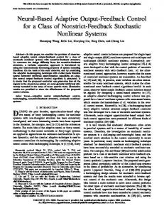
can stabilize the plant. Second, we invoke Lemma 1 (see Appendix), which shows that a stabilizing multiple-derivative controller can always be approximated by a multiple-delay controller that is also stabilizing. In particular, we from the lemma that �see M a controller of the form u(t) = i=1 Ki y(t − ǫτi ), where 0 ≤ τ1 < τ2 < ... < τM and ǫ is a small positive constant can stabilize the plant. We thus recover that the result of the Theorem, choosing τ¯i = ǫτi . � If the plant is not square-invertible, then design of a multiple-delay controller can be achieved through squaringdown followed by application of the above result for squareinvertible plants. Specifically, in this case, an (in general dynamic) open-loop precompensator and postcompensator can be applied to construct a square-invertible and minimumphase plant, see [9] and also Figure 1. In turn, the multiple-
419
Kpre (s)
Non−square− invertible plant
Kpost (s)
Fig. 1. A minimum-phase non-square-invertible plant can be made minimum-phase square-invertible using (in general dynamic) pre- and postcompensation. We can thus develop multiple-delay controllers even in the non-square-invertible case.
delay controller design for minimum-phase plants can be applied. We stress here that in many cases static pre- and post-compensation can be used, in which case the form of the controller is exactly as in Theorem 1. We also note that the pre- and post-compensation do not change the infinite zero structure of the plant (see [9]), so the number of delays needed by the controller is identical to the number in squareinvertible case. III. N ON -M INIMUM P HASE P LANTS At their essence, the multiple-delay controllers proposed in the literature use delayed observations to estimate derivatives of the output. The SCB formulation above clarifies that these derivatives contain (partial) state dynamics of the systems, and hence are valuable for control. However, it is classically known, and can be seen from the SCB, that derivatives of the output do not contain the zero dynamics of the plant. We thus expect that non-minimum-phase plants will not generally be stabilizable by multiple-derivative or multiple-delay controllers. Let us first give two examples, one of a non-minimum phase plant that can be stabilized using multiple-delay control and one of a non-minimum-phase plant that cannot be stabilized by any multiple-derivative linear controller (and hence also cannot be stabilized by a controller that approximates derivatives using delays). After presenting the examples, we will clarify that the problem of stabilizing a general plant with multiple delays (or derivatives) can be phrased as a static controller design problem, and hence the wide literature on static stabilization [10] can be applied. Example 1: The non-minimum phase SISO plant with transfer s−1 can be stabilized using a function H(s) = s2 (s+10) 2 multiple-delay feedback controller. To verify, notice that a feedback controller that uses two derivatives of the output, 2 namely u(t) = ddt2y + 2 dy dt + y, stabilizes the plant. We thus can construct a controller that uses three delayed observations to stabilize the plant, as by approximating the derivatives using delay differences. Example 2: 3 A SISO plant with transfer function H(s) = (s−1) s4 cannot be stabilized by any multiple-derivative �Nfeedback (i) controller, i.e. any controller of the form u = i=0 αi y , for any N . To see this, notice that the controller’s transfer function is a degree-N polynomial, say p(s). Let us first
consider the case that p(s) has no zeros at the origin. In this case, the characteristic polynomial of the closed-loop is easily seen to be s4 + (s − 1)3 p(s). Noticing that (s − 1)3 p(s) is a polynomial with three positive real roots, its coefficients have at least three sign changes according to Descartes’ classical rule of signs. Thus, the coefficients of the closed-loop characteristic polynomial s 4 + (s − 1)3 p(s) change signs at least once (since s 4 is a monomial and so changes only one coefficient in the polynomial), all roots cannot be in the OLHP. In the case where p(s) has zeros at the origin, the characteristic polynomial of the closed-loop takes the form s j + (s − 1)3 p�(s) where j = 0, 1, 2, 3 and p�(s) is formed from p(s) by removing 4 − j roots at the origin. Thus, by exactly the same argument, we see that not all roots of the characteristic polynomial are in the OLHP, and stability cannot be achieved. We note that this example shows that multiple-derivative controllers cannot generally be used to stabilize nonminimum-phase plants. Since the known methods for multiple-delay control are based on approximating derivatives using delay differences, these methods unfortunately cannot in general be used to stabilize non-minimum-phase plants. More fundamentally, we contend that multiple-delay controllers are essentially equivalent to multiple-derivative controllers, and so we conjecture that no multiple-delay controller can stabilize this plant either. The above two examples suggest that some but not all non-minimum phase plants can be stabilized using multiplederivative and hence multiple-delay controllers. Thus, we are motivated to find ways for distinguishing plants that can and cannot be stabilized by multiple-delay controllers. In fact, we can straightforwardly pose this classification problem as a static stabilizability problem. Let us present this formalization for the case of SISO plants (for simplicity). Theorem 2: Consider a SISO LTI plant with n poles and m zeros, and consider another (SIMO) plant with the same state equation but with the output appended by its first n − m − 1 derivatives. If this (virtual) SIMO plant can be stabilized using a static linear feedback controller, then the SISO plant can be stabilized using a controller that uses n − m delays. The proof of this theorem is immediate: static stabilizability of the SIMO plant implies stabilizability of the SISO plant using feedback that is a linear combination of the first n−m−1 derivatives of the output (and in turn stabilizability using multiple-delay control, see Appendix). We note that only n − m − 1 derivatives (equivalently, n − m delays) are considered, since higher derivatives of the output involve the input and hence cannot always be computed/approximated in practice, nor can such controllers based on higher derivatives always be approximated using multiple-delay controllers. The theorem generalizes naturally to the MIMO case. Specifically, through an appropriate transformation, we
420
can view the infinite zero dynamics as comprising multiple coupled integrator chains whose outputs are linear combinations of the original plant’s outputs. By appending the output with derivatives of each of these linear combinations up to one less than the depth of the corresponding integrator chain (i.e., the maximum order of the infinite zeros associated with this chain), we can pose the multiple-derivative controller design as a static controller design problem for the appended system. We thus recover that multiple-delay controllers can be designed whenever this static controller design problem can be solved. Remark: We note that that the system with extended output as given above has the same spectrum and blocking-zero structure as the original plant. It follows immediately that a necessary condition for the multiple-derivative control and hence our multiple-delay control is that the parity interlacing property holds, e.g. [10], [11]. Acknowledgements We thank Professor A. Stoorvogel for several illuminating discussions on the spectra of delay-differential equations. This work was partially supported by the National Science Foundation under Grant ECS-0528882 and by the National Aeronautics and Space Administration under Grant NNA06CN26A. R EFERENCES [1] J. K. Hale and S. M. V. Lunel, Introduction to Functional Differential Equations, Springer-Verlag: New York, 1993. [2] S.-I. Niculescu and W. Michiels, “Stabilizing a chain of integrators using multiple delays,” IEEE Transactions on Automatic Control, vol. 49, no. 5, pp. 802-807, May 2004. [3] V. L. Kharitonov, S.-I. Niculescu, J. Moreno, and W. Michiels, “Static output feedback stabilization: necessary conditions for multiple-delay controllers,” IEEE Transactions on Automatic Control, vol. 50, no. 1, pp. 82-86, Jan. 2005. [4] A. Ilchmann and C. J. Sangwin, “Output feedback stabilization of minimum phase systems by delays,” Systems and Control Letters, vol. 52, pp. 233-245, 2004. [5] P. Sannuti and A. Saberi, “A special coordinate basis of multivariable linear systems, finite and infinite zero structure, squaring down, and decoupling,” International Journal of Control, vol. 45, no. 5, pp. 16551704, May 1987. [6] A. Saberi and P. Sannuti, “Time-scale structure assignment in linear multivariable systems with high-gain feedback,” International Journal of Control, vol. 49, no. 6, 1989. [7] A. Saberi, B. M. Chen, and P. Sannuti, Loop Transfer Recovery: Analysis and Design, Springer-Verlag, 1993. [8] X. Liu, Z. Lin, and B. M. Chen, “Symbolic realization of asymptotic time-scale and eigenstructure assignment design method in multivariable control,” International Journal of Control, vol. 79, no. 11, pp. 1471-1484, Nov. 2006 [9] A. Saberi and P. Sannuti, “Squaring down by static and dynamic compensators,” IEEE Transactions on Automatic Control, vol. 33, no. 4, Apr. 1988. [10] V. I. Syrmos, C. T. Abdallah, P. Dorato, and K. Grigoriadis, “Static output feedback–a survey,” Automatica, vo. 33, no. 2, pp. 125-137, 1997. [11] D. C. Youla, D. D. Bongiorno Jr., and C. N. Liu, “Single loop feedback stabilization of linear multivariable plants,” Automatica, vol. 10, pp. 159-173, 1974. [12] W. Michiels and T. Vyhlidal, “An eigenvalue based approach for stabilization of linear time-delay systems of neutral type,” Automatica, vol. 41, pp. 991-998, 2005.
[13] W. Michiels and D. Roose, Global stabilization of multiple integrators with time-delay and input constraints, Technical Report TW 325, Department of Computer Science, K.U.Lueven. [14] A. Papoulis, “Limits on bandlimited signals,” Proceedings of the IEEE, vol. 55, no. 10, pp. 1677-1686, Oct. 1967.
A PPENDIX We show in this appendix that a multiple-delay controller can be designed to stabilize an LTI plant whenever a multiple-derivative controller of the form given in Equation 1 can be used to stabilize the plant. The stability of a delay-differential equation, such as the closed-loop system in our case, is usually proved using either the RazhumikinLyapunov theory (which connects the time-evolution of a Lyapunov function to that of an interval-maximum functional) or directly using Lyapunov-Krakovskii functionals [1]. The argument that we use here is essentially of the Razhumikhin-Lyapunov type, though we find it preferable to work directly with an interval-maximum functional than to use a Lyapunov function and subsequently connect it to the functional. Specifically, we prove stability using a quadratic functional of the from C(t) = max τ ∈[0,MǫτM ] x(t − τ )P x(t − τ ) where τM is the maximum delay used in the multiple-delay controller. Fundamentally, the equivalence between multiplederivative control and multiple-delay control is evident: because we have the freedom to choose the delays arbitrarily small, the closed-loop trajectory upon multiple-delay control can be made to approximate that achieved by multiplederivative control (at least as long as the feedback does not include delayed derivatives of the state itself, see e.g. [12] for further discussion of these complicated neutral delay-differential equations). In turn the functional can be shown to be non-increasing and attractive. This result is formalized below. Lemma 1: Consider a SISO LTI plant with relative degree M can be stabilized by the �Mthat (i−1) k y (t). Then the controller controller u = i i=1 �M �M (j−1)!kj dQ u(t) = i=1 Ki y(t − ǫτi ), where Ki = j=1 ǫj−1 det(Q)i,j , 1 τ1 ... τ1M−1 1 τ2 ... τ2M−1 Q = . .. .. , and dQi,j is the (i, j)th .. . ... . M−1 1 τM ... τM minor, also stabilizes the plant for sufficiently small ǫ 1 . Proof: We will prove stability using a Lyapunov functional of the form V (t) = maxs∈[0,MǫτM ] xT (t−s)P x(t−s). Specifically, we shall show that V (t) is not only non-increasing but also attractive to the origin, and hence we shall prove stability (see e.g. [1]). We broadly follow the approach taken by Michiels and Roose [13], but prove asymptotic stability in addition to invariance of the closed-loop system, and also 1 We note that the gains in the multiple-delay controller are based on approximating the observation y(t) with a polynomial interpolation over the interval [0, ǫτM ], see [2] for details.
421
extend their argument to the multiple-delay case. The proof is organized as follows: first, we formalize that the closed-loop dynamics can be viewed as a stable finite-state LTI dynamics plus a small delay-based correction term that results from the approximation of derivatives with delays. Using this formulation, we specify a Lyapunov functional that can be used to 1) prove invariance of particular Lyapunov balls of arbitrary size, and 2) show that the functional and hence the state is attractive to the origin. This attractivity proof is based on a bound on the time by which the the state enters a smaller invariant set. First, let us express the closed-loop system dynamics when the multiple-delay controller is used in terms of the closed-loop dynamics upon multiple-derivative control, plus an error. For convenience, let us first define an extended y y˙ output vector y ˜ = .. . In this notation, the input .
y (M−1) u(t) when the multiple-delay controller is used can be written as the input when multiple-derivative control is used (which constitutes a static linear feedback of y ˜), plus a (small) correction term that captures the difference between multiple-delay-based approximation of output derivatives and T ˜+k ˜dif f , the derivatives themselves. That is, u(t) =k T y y yapp . ˜app − y ˜, where y ˜app = .. , where where y ˜dif f = y (M−1)
yapp is the approximation of the ith derivative of y using i+1 T � delays as in the Lemma statement, and k = k1 ... kM . We notice that our approximation for the ith derivative (y (i) ) is constructed by interpolating the observation y(t) at i + 1 points on the interval [t − ǫτ i , t]. We note that, from the classical mean value theorem for divided differences, there (i) exist θi ∈ [0, ǫτi ], i ∈ 1, . . . , n such that y (i) (t) − yapp (t) = (i+1) ǫτi y (t − θi ); we shall use this fact subsequently to show that the functional is non-increasing and attractive. Using the re-written observation vector, we can straightforwardly express the closed-loop dynamics as x˙ = Ax + ˜ for appropriate C˜ bkT (˜ y+y ˜diff ). Noting that y ˜ = Cx (since, from the SCB, each of the first M derivatives of y(t) can be written as linear combinations of x(t)), we obtain ˜ + bkT y ˜diff . We note here that that x˙ = (A + bkT C)x A = A + bkT C˜ is Hurwitz stable, and so there exists P > 0 T and Q > 0 such that A P + P A ≤ −Q. Let us now prove stability of the closed-loop system using the functional V (t) = maxs∈[0,MǫτM ] xT (t − s)P x(t − s). We do so from first principles, in two steps: 1) we show that V (t) is a non-increasing function of time, and 2) we show that V (t) approaches 0 (in fact exponentially) by bounding the times at which V (t) is less than arbitrary fractions of its initial value. To show that V (t) is non-increasing, let us first show that if V (� t) = c, then V (t) ≤ c for t ≥ � t, for any c (when ǫ is chosen sufficiently small). From the fact that V ( � t) = c, (i) yapp
we know that W (t) = xT (t)P x(t) is less than or equal to c t. From continuity of the solution, we for � t − M ǫτM ≤ t ≤ � thus know that there must be a particular time t such that W (t) = c for the first time if c is to be exceeded, and further W () must increase from less than c to greater than c at this ˙ is time t. We prove this is impossible by showing that W less than 0 for W (t) = c, and hence prove that V (t) ≤ c for t≥� t. Specifically, note that T ˙ = xT (AT P + P A)x + xT P bkT y ˜diff + y ˜diff kbT P x. W (2) Hence, ˙ ≤ −xT Qx + 2|x||P bkT y W ˜diff |. (3) ǫτ1 y (1) (t − θ1 ) ǫτ2 y (2) (t − θ2 ) We recall that y ˜diff (t) = , for some .. . (M) (t − θM ) ǫτM y θ1 , . . . , θM . Substituting, we obtain that
ǫτ1 y (1) (t − θ1 )
ǫτ2 y (2) (t − θ2 )
T T ˙ ≤ −x Qx + 2|x||P bk | W
. (4) ..
.
ǫτM y (M) (t − θM )
Note that ǫτi y (i) (t−θi ) are clearly bounded linearly with the norm of x(t−θ i ) and with ǫ for i = 1, . . . , M 1 , since each of these derivatives is a linear function of the concurrent state. However, further effort is needed in bounding ǫτ M y (M) (t − θM ). To continue, notice that this term can be rewritten as ˙ − θM )) = ǫτM C(M−1) (Ax(t − θM ) + ǫτM C(M−1) x(t ˜ app (t−θM )), where C(M−1) describes the linear transbkT y formation from x to y (M−1) . Notice that ǫτM C(M−1) Ax(t− θM ) is guaranteed to be bounded by a function that is linear ˜ app (t − with ǫ and with the norm of x(t − θ M ), but bkT y θM )) requires more work to bound since the approximation ˜ app (t − θM ) depends on ǫ. Let us thus study this term a bit y ˜ app (t−θM )) can be rewritten further. In particular, note that y ˜ (t − θM ) + y ˜ dif f (t − θM ). The first ˜ app (t − θM ) = y as y ˜ (t−θM ) is bounded. The second term, y ˜ dif f (t−θM ) term, y ˜dif f(t), specifcan be approximatedin the same way as y ǫτ1 y (1) (t − θM − φ1 ) ǫτ2 y (2) (t − θM − φ2 ) ically as y ˜diff (t) = , for some .. . (M) (t − θM − φM ) ǫτM y φ1 , . . . , φM . Here, all terms are guaranteed to be bounded with respect to ǫ and the norm of x at the appropriate time, except the highest-order one. However, substituting this ˙ , we finally highest-order term into the expression for W recover that the only (possibly) unbounded term has the form ǫ2 qy(M) (t − θM − φM ), where q is a fixed constant. Repeating this process M − 2 further times, we finally recover that the only (possibly) unbounded term has the form ǫM ry(M) (t − θbig ), where θbig < M ǫτM and r is a fixed constant.
422
˙ we obtain that Finally, noting that y (M) = C(M−1) x, ˙ − θbig ) = ǫM rC(M−1) (Ax(t − this term is ǫM rC(M−1) x(t θbig ) + bu(t − θbig )). The first of the two terms in the above expression is clearly bounded with ||x|| and ǫ (in fact, ǫM ). Meanwhile, from the expression for the multiple-delay controller, we see that u(t − θ big ) can be bounded by ǫMC−1 for some positive constant C (for x in the given ball). Thus, we recover that ǫ M rC(M−1) Ax(t − θbig ) + bu(t − θbig ) is bounded by a linear function of ǫ and the norm of x. Hence, ˙ from that we have finally proved that the perturbation of W upon use of a multiple-derivative controller (see Equation 2) can be bounded by a sum of terms that are each linear with ǫ, and with a norm of x for a time between 0 and M ǫτ M . In turn, we recover that ˙ ≤ −λmin (Q)|x|2 + ǫL|x|2 , W
(5)
where the positive constant L (which does not depend on c) (Q) , is not worth our while to compute. By choosing ǫ < λmin L we can guarantee that the derivative of W (t) is negative for W (t) = c, and hence W (t) and in turn V (t) do not exceed c. Since this statement holds for all c, we automatically recover that V (t) is a non-increasing function of time. We can straightforwardly extend the above argument to show that the functional V (t) not only is non-increasing but in fact approaches 0. In particular, we can prove the (P ) + M ǫτM ) ≤ following: if V (� t) = c, then V (� t + 2 λλmax min (Q) (Q) as long as we choose ǫ < λmin (where L is the 4L positive constant described above). To prove this, simply note that by choosing ǫ in this way and using the fact that the norms of the delayed versions of x are bounded c max (P ) by 2λ λmin (P ) |x(t)| while W (t) is between 2 and c, we ˙ ≤ − 1 λmin (Q)|x|2 . Thus, while c ≤ guarantee that W 2 2 W (t) ≤ c, it is guaranteed that W (t) decreases at a rate 1 λmin (Q) c min (Q) of at least 12 λmin (Q)|x|2 ≥ 12 λλmax (P ) W (t) ≥ 2 λmax (P ) 2 . We thus recover that W (t) can remain between c and 2c for a (P ) . Once W (t) has dropped below maximum time of 2 λλmax min (Q) c , it is clear from the fact that the derivative is negative for 2 W (t) ≥ 2c that V (t) cannot again exceed 2c . Thus, we recover the result above. Repeating the argument, we obtain that (P ) V (t) ≤ 2cn for t ≥ � +nM ǫτM , and so we have t +2n λλmax min (Q) proved asymptotic (and in fact exponential) convergence of the state to the origin. We have thus proved that, if the state is upper-bounded by a constant c over the interval [−M ǫτ M , 0], then it is bounded c 2,
by c for all t ≥ 0 and in fact converges exponentially to the origin. The only remaining step in proving stability (see e.g. [1]) is to show that boundedness over the shorter interval [−ǫτM , 0] yields boundedness and convergence. However, it is trivial to show through a scaling argument that the shorter interval suffices. � While the above proof is tedious, the underlying concept is rather simple: using small delays, we can approximate the multiple-derivative control arbitrarily closely, and hence the response when the multiple-delay controller is used is close to the response when the multiple-derivative controller is used, for finite time periods. Since the multiple-derivative controller is asymptotically stable, it is decrescent with respect to a particular Lyapunov function; the associated Lyapunov functional can thus be shown to be decrescent over periods of time when the multiple-delay controller is used, and in turn stability can be proved. The result generalizes naturally to the MIMO case. We can approximate all the required derivatives of the the output (specifically, of linear combinations of output variables), as delay differences. Again, as we make the delays small, we find that the multiple-delay controller approximates the multiple-derivative controller more and more accurately, and hence an identical Lyapunov argument suffices to prove stability—the only difference is that the observation and its required derivatives are vectors (rather than scalars) that depend linearly on the state and its derivative. Since the highest derivative used by the controller is the maximum M among the orders of the infinite zeros minus 1, we recover that M − 1 + 1 = M delays are needed. A couple further notes about the multiple-delay approximation are worthwhile. First, the above argument can straightforwardly be extended to show that the Lyapunov exponent for the multiple-delay control can be made arbitrarily close to that for the multiple-derivative control. Second, it can be shown that the finite poles of the multipledelay-controlled system approach the poles of the multiplederivative-controlled system, while the additional poles move toward −∞ as ǫ becomes small. A full treatment of this second point is deferred to future work. We also leave it to future work to select the delays τ 1 , . . . , τM , so as to trade off accuracy in the derivative approximation (and hence in the settling response) with robustness to additive noise, see e.g. [14] for relevant analysis.
423