On solving sparse algebraic equations over finite fields II

On solving sparse algebraic equations over finite fields II Igor Semaev Department of Informatics, University of Bergen, Norway

Abstract. A system of algebraic equations over a finite field is called sparse if each equation depends on a small number of variables. Finding efficiently solutions to the system is an underlying hard problem in the cryptanalysis of modern ciphers. In this paper deterministic AgreeingGluing algorithm introduced earlier in [9] for solving such equations is studied. Its expected running time on uniformly random instances of the problem is rigorously estimated. This estimate is at present the best theoretical bound on the complexity of solving average instances of the above problem. In particular, it significantly overcomes our previous results, see [11]. In characteristic 2 we observe an exciting difference with the worst case complexity provided by SAT solving algorithms.

Keywords: sparse algebraic equations over finite fields, constraint satisfaction problem, agreeing, gluing.

1

Introduction

Let (q, l, n, m) be a quadruple of natural numbers, where q is a prime power. Then Fq denotes a finite field with q elements and X = {x1 , x2 , . . . , xn } is a set of variables from Fq . By Xi , 1 ≤ i ≤ m we denote subsets of X of size li ≤ l. The system of equations f1 (X1 ) = 0, . . . , fm (Xm ) = 0

(1)

is considered, where fi are polynomials over Fq and they only depend on variables Xi . Such equations are called l-sparse. We look for the set of all solutions in Fq to the system of equations (1). Therefore, we can only consider for fi polynomials of degree at most q − 1 in each variable or, in other words, the exponent in each variable is at most q − 1. The polynomial fi defines a mapping from the set of all li -tuples over Fq to Fq and vice versa any such mapping may be represented by a polynomial over Fq of degree at most q − 1 in each variable. Obviously, the equation fi (Xi ) = 0 is determined by the pair (Xi , Vi ), where Vi is the set of Fq -vectors in variables Xi , also called Xi -vectors, where fi is zero. Following terminology in [9], we also call the pair (Xi , Vi ) a symbol. For q = 2 the polynomial fi is uniquely defined by Vi . Given fi , the set Vi is computed with q li trials. Solving (1) may be considered as a Constraint Satisfaction Problem, see [12], with constraints given by Vi .

In this paper deterministic Agreeing-Gluing Algorithm, introduced in [9] and aimed to find all solutions to (1), is studied and its average behavior is estimated. To this end equiprobable distribution on instances (1), each instance has the same probability, is assumed. That is, given the sequence of natural numbers m and l1 , . . . , lm ≤ l, equations in (1) are generated independently. The particular equation fi (Xi ) = 0 is determined by the subset Xi of size li taken uniformly at from the set of all possible li -subsets of X, that is with the probability ¡random ¢ li n −1 , and the mapping (polynomial) fi taken with the equal probability q −q li from the set of all possible mappings to Fq defined on li -tuples over Fq (the set of polynomials of degree ≤ q − 1 in each of li variables). In this setting the running time of the Agreeing-Gluing Algorithm is a random variable. We estimate its expected complexity. For fixed q, l and c ≥ 1 let β = β(α), where 0 ≤ α ≤ l, be the only root to the equation q

β− αl

g(α)

= qe

l µ ¶ X α l l−t 1 t (1 − β (1 − β)t (1 − )q )c− l , q t t=0

or β(α) = 0 if there is not any root for some α. Here g(α) = f (zα ) − α + α ln α − α ln q and f (z) = ln(ez + q −1 − 1) − α ln(z), where by zα we denote the only l positive root of the equation ∂f ∂z (z) = 0. We realize that the above equation doesn’t depend on n. We prove m Theorem 1. Let l1 +l2 +...+l tend to a constant c ≥ 1 as n tends to ∞ while ln q ≥ 2 and l ≥ 3 are fixed. Let r(q, l, c) be the maximal of the numbers α

max q β(α)− l

0≤α≤l

and

1.

Then the expected complexity of the Agreeing-Gluing Algorithm is O((r(q, l, c) + ε)n ) bit operations for any positive real number ε. For any triple q, l, c ≥ 1 the Theorem enables estimating the expected running time of the Agreeing-Gluing Algorithm with some mathematical software like Maple. To this end we realize that the equation ∂f ∂z (z) = 0 is equivalent to zez = α. So α = α(z) and β = β(z) are found to be functions in z and z −1 e +q −1 zα = z. We did the computation with Maple for some of 2, l, 1(e.g. n Boolean equations in n variables each equation depends on l variables) and show the data obtained in Table 1 along with the expected complexities of the Gluing1 and Gluing2 Algorithms from our previous work [11]. Agreeing-Gluing1 Algorithm is a variant of the Agreeing-Gluing Algorithm with the same asymptotical running time and polynomial in n memory requirement. We have shown in [11] that in case q = 2 each instance of (1) may be encoded with a CNF formula in the same set of variables and of clause length at most l. Therefore, l-SAT solving algorithms provide with the worst case complexity estimates found e.g. in [5].

So in the first line we show the worst case estimates for (1) too. We remark an exciting difference in the worst case complexity and expected complexity of the Agreeing-Gluing Algorithm. It is quite obvious that average instances of the Table 1. Algorithms’ running time. l the worst case Gluing1, expectation Gluing2, expectation Agreeing-Gluing1, expectation

3 1.324n 1.262n 1.238n 1.113n

4 1.474n 1.355n 1.326n 1.205n

5 1.569n 1.425n 1.393n 1.276n

6 1.637n 1.479n . 1.446n 1.334n

l-SAT problem and that of (1) are different. That gives insight into why the expected complexity is so low in comparison with the worst case. In case of n Boolean equations (q = 2) of algebraic degree d in n variables defining a so called semi-regular system( it was conjectured, see [1], but not proved that an average instance of the problem behaves semi-regularly) the running time of the popular Gr¨obner Basis Algorithm and its variants, e.g. [2] and [4], is known. For d = 2, one gets the bound O(1.7n ) by guessing a number of variables before the Gr¨obner Basis Algorithm (or XL) application, see [13]. For d ≥ 3 the bounds exceed the cost of the brute force algorithm, that is 2n . Thus the Agreeing-Gluing family algorithms seem better on sparse equation systems (1) than the Gr¨obner Basis related algorithms. This article was motivated by applications in cryptanalysis. Modern ciphers are product, that is the mappings they implement are compositions of functions in small number of variables. Then intermediate variables are introduced in order to simplify equations, describing the cipher, and to get a system of sparse equations. E.g., given one pair of plain-text, cipher-text blocks, DES is described by 512 Boolean equations in 504 variables, each equation involves at most 14 variables, see [9]. For a more general type of sparse equations, Multiple Right Hand Side linear equations describing in particular AES, see [10]. Solving such systems of equations breaks the cipher. Here we are studying an approach which exploits the sparsity of equations and doesn’t depend on their algebraic degree. This approach was independently discovered in [14] and [8], where the Agreeing procedure was described for the first time. The term Agreeing itself comes from [9]. The Agreeing procedure was in these works then combined with guessing some of the variables values to solve (1). That makes somewhat similar to the Agreeing-Gluing1 Algorithm of the present paper. However no asymptotical estimates for that type of algorithms were given in [14, 8, 9]. It is often important in cryptology to understand the hardness of average instances of the computational problem under question rather than its worst case complexity. So the present paper, like [11], focuses on the expected performance of the algorithms. The rest of the paper is organized as follows. In Sections 2 Gluing procedure and the Gluing Algorithm are presented. The Agreeing procedure and the

Agreeing-Gluing Algorithm are described in Section 3. Section 4 presents the Agreeing-Gluing1 Algorithm and in Section 5 asymptotic bound on its running time, that is Theorem 1, is proved. Before reading this paper, we recommend to look through our previous work [11], where some necessary basic facts were proved. For the reader’s convenience we also formulate them in Section 2. The author is grateful to H.Raddum for careful reading this work and numerous remarks.

2

Gluing procedure and Gluing Algorithm

We describe the Gluing procedure. Given symbols (Xi , Vi ) for i = 1, 2, one defines two sets of variables Z = X1 ∪ X2 and Y = X1 ∩ X2 and a set of Zvectors U by the rule U = {(a1 , b, a2 ) : (a1 , b) ∈ V1 , (b, a2 ) ∈ V2 }, where ai is an (Xi \ Y )-vector and b is a Y -vector. We denote (a1 , b, a2 ) = (a1 , b) ◦ (b, a2 ) and say that (a1 , b, a2 ) is the gluing of (a1 , b) and (b, a2 ). In order to glue (X1 , V1 ) and (X2 , V2 ) one can sort V1 or V2 by Y -subvectors and only glues vectors with the same Y -subvector. So the complexity of the gluing is O(|U | + (|V1 | + |V2 |) log(|Vi |))

(2)

operations, as rewriting and comparison, with Fq -vectors of length at most |Z|, where |Vi | are big enough. We actually use a simpler bound O(|V1 ||V2 |+|V1 |+|V2 |) in what follows. We denote (Z, U ) = (X1 , V1 ) ◦ (X2 , V2 ). Gluing Algorithm input: the system (1) represented by symbols (Xi , Vi ), where 1 ≤ i ≤ m. output: the set U of all solutions to (1) in variables X(m) = X1 ∪ . . . ∪ Xm . put (Z, U ) ← (X1 , V1 ) and k ← 2, while k ≤ m do (Z, U ) ← (Z, U ) ◦ (Xk , Vk ) and k ← k + 1, return (Z, U ). It is obvious that U is the set of all solutions to (1) in variables X(m). Example. For the system x1 x2 a1 0 0 , a2 1 0 a3 1 1

x2 x3 b1 0 0 , b2 1 0 b3 1 1

x1 x3 c1 0 0 c2 0 1

the Algorithm computes two gluings: x1 0 1 1

x1 x2 x2 x3 0 0 0 0 ◦ = 1 0 1 0 1 1 1 1 1

x2 0 0 1 1

x3 0 0, 0 1

x1 0 1 1 1

x2 0 0 1 1

x3 0 x1 x3 x x x 0 ◦ 0 0 = 1 2 3. 0 0 0 0 0 1 1

So there is only one solution (x1 , x2 , x3 ) = (0, 0, 0). The Gluing Algorithm takes O(

m−1 X

m−1 X

|Uk ||Vk+1 | + |Uk | + |Vk+1 |) = O(

k=1

|Uk | + m)

(3)

k=1

operations with Fq -vectors of length at most n, where q and l are fixed, and n or m may grow. The memory requirement is of the same magnitude as the running time. Here (X(k), Uk ) = (X1 , V1 ) ◦ . . . ◦ (Xk , Vk ) and (3) is the cost of m − 1 gluings. The set Uk consists of all solutions to the first k equations in variables X(k) = X1 ∪ . . . ∪ Xk . The sequence of |Uk | fully characterizes the running time (3) of the algorithm. The asymptotical analysis of |Uk | and the Gluing Algorithm is done in [11] using Random Allocations Theory results found in [7, 6, 3]. In [11] the following Theorem was proved: Theorem 2. Let ² be any positive real number, l ≥ 3 and q ≥ 2 be fixed natural numbers as n or m tend to infinity. Then the expected complexity of the Gluing Algorithm is O((q 1−γq,l + ²)n + m) bit operations, where γq,l = 1 1−q −1 1 l ). −1 l + (q − 1) logq ( 1−q

l

Two technical statements from [11] are formulated. We use them in Section 5. Lemma 1. (Lemma 4 in [11]) Let the subsets of variables X1 , . . . , Xk be fixed while f1 , . . . , fk are randomly chosen according to our model. Then the expected number of solutions to the first k equations in (1) is Ef1 ,...,fk |Uk | = q |X(k)|−k . Lemma 2. (Lemma 5 in [11]) Let Lk = l1 + . . . + lk and α = Lk /n, and k ≤ n. Let 0 < δ < 1 be fixed as n tends to ∞. Then the expected number of solutions to the first k equations is ½ δ < qn , if Lk < nδ ; E|Uk | = EX1 ,...,Xk (q |X(k)|−k ) = g(α) n O((qe + ²) ), if Lk ≥ nδ , q and for any positive real number ². Here g(α) = f (zα ) − α + α ln α − α ln l z −1 f (z) = ln(e + q − 1) − α ln(z), where by zα we denote the only positive root of the equation ∂f ∂z (z) = 0.

3

Agreeing procedure and Agreeing-Gluing Algorithm

We describe the Agreeing procedure. Given symbols (Xi , Vi ) for i = 1, 2, one defines the set of variables Y = X1 ∩X2 . Let V1,2 be the set of Y -subvectors of V1 . In other words, that is the set of projections of V1 to variables Y . Similarly, the set V2,1 of Y -subvectors of V2 is defined. We say the symbols (X1 , V1 ) and (X2 , V2 ) agree if V1,2 = V2,1 . Otherwise, we apply the procedure called agreeing. We delete from Vi all vectors whose Y -subvectors are not in V2,1 ∩V1,2 . Obviously, we delete

Vi -vectors which can’t make part of any common solution to the equations. So new symbols (Xi , Vi0 ) are determined, where Vi0 ⊆ Vi consist of the vectors in Vi survived after agreeing. We finally put (Xi , Vi ) ← (Xi , Vi0 ). In order to agree (X1 , V1 ) and (X2 , V2 ) one sorts V1 or V2 by Y -subvectors and do agreeing by table look ups. So the complexity of the agreeing is at most O((|V1 | + |V2 |) log(|Vi |))

(4)

operations, as rewriting and comparison, with Fq -vectors of length at most n, where |Vi | are big enough. For instance, we agree the first and the third equations in the example. x1 x2 a1 0 0 (X1 , V1 ) = , a2 1 0 a3 1 1

x1 x3 (X3 , V3 ) = c1 0 0 . c2 0 1

Then one defines Y = {x1 } and V1,3 = {0, 1}, and V3,1 = {0}. Therefore, a2 and a3 should be deleted from V1 . The new agreed symbols are (X1 , V1 ) =

x1 x3 (X3 , V3 ) = c1 0 0 . c2 0 1

x1 x2 , a1 0 0

The following Agreeing-Gluing Algorithm combines the Agreeing and Gluing procedures to solve (1). Agreeing-Gluing Algorithm input: the system (1) represented by symbols (Xi , Vi ), where 1 ≤ i ≤ m. output: the set U of all solutions to (1) in variables X(m) = X1 ∪ . . . ∪ Xm . put (Z, U ) ← (X1 , V1 ) and k ← 2, while k ≤ m do s ← k, while s ≤ m agree (Z, U ) and (Xs , Vs ), put s ← s + 1, put (Z, U ) ← (Z, U ) ◦ (Xk , Vk ) and k ← k + 1, return (Z, U ). We introduce some notation. Let (X(1), U10 ) be the symbol (X1 , V1 ) after m − 1 agreeings with the symbols (Xi , Vi ), where 1 < i ≤ m. Generally, for any 1 ≤ 0 k < m let (X(k + 1), Uk+1 ) denote the symbol (X(k), Uk0 ) ◦ (Xk+1 , Vk+1 ) after agreeing with (m − k − 1) symbols (Xi , Vi ), where k + 1 < i ≤ m. It is easy to see that the Agreeing-Gluing Algorithm produces the sequence of (X(k), Uk0 ). For the above example the sequence of such symbols is (X(1), U10 ) =

x1 x2 , 0 0

(X(2), U20 ) =

x1 x2 x3 , 0 0 0

(X(3), U30 ) =

x1 x2 x3 , 0 0 0

where X(1) = {x1 , x2 } and X(2) = X(3) = {x1 , x2 , x3 }. One sees that the Agreeing-Gluing Algorithm takes m−1 X

O(

|Uk0 ||Vk+1 | + |Uk0 | + |Vk+1 | + (m − k − 1)|Uk0 ||Vk+1 |) =

k=1

O(m(

Pm−1 k=1

|Uk0 | + 1))

(5)

operations with Fq -vectors of length at most n, where q and l are fixed, and n or m may grow. The formula (5) incorporates the cost of the gluing (X(k), Uk0 ) ◦ (Xk+1 , Vk+1 ), which is O(|Uk0 ||Vk+1 | + |Uk0 | + |Vk+1 |) = O(|Uk0 |) operations, and the agreeing the resulting set of X(k + 1)-vectors, of size at most |Uk0 ||Vk+1 | = O(|Uk0 |), with the rest m−k −1 symbols. In our setting |Uk0 | is a random variable. We estimate the expectation of |Uk0 | in Section 5, see Theorem 3. That will imply Theorem 1. The memory requirement of the Agreeing-Gluing Algorithm is of the same magnitude as the running time, but the Agreeing-Gluing1 Algorithm in the next Section only requires polynomial memory while its asymptotical running time is the same. From the definition of Gluing and Agreeing procedures we also get the following statement. Lemma 3. (X(k), Uk0 ) is the symbol (X(k), Uk ) = (X1 , V1 ) ◦ . . . ◦ (Xk , Vk ) after agreeing with (m − k) symbols (Xi , Vi ), where k < i ≤ m.

4

Agreeing-Gluing1 Algorithm

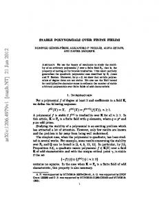
The Gluing1 Algorithm in [11] has the same time complexity as the Gluing Algorithm and only requires poly(n) bits of memory. The Algorithm walks through a search tree with backtracking. The complexity is roughly the number of the tree branches. The search tree for the above example is depicted in Fig.1, where a1 ◦ b1 ◦ c1 = (0, 0, 0) is the only solution.

Fig. 1. The search tree for the Gluing1 Algorithm.

Similarly, the Agreeing-Gluing1 Algorithm is a variant of the Agreeing-Gluing Algorithm with minor memory requirements. In order to define the related search tree we say that an X(k)-vector a contradicts(does not agree) with the symbol (Xi , Vi ), where i > k, if the projection of a to the common variables X(k) ∩ Xi is not in the projections of Vi to the same variables. In this case a can’t be the part of any solution to the system. A rooted search tree is now being defined. The root, labeled by ∅, is connected to nodes at level 1, labeled by elements of V1 which do not contradict with the

symbols (Xi , Vi ) for all i > 1. Nodes at level k ≥ 2 are labeled by some of b ∈ Vk . A node at level 1, labeled by a, is connected to a node at level 2, labeled by b, whenever the gluing a ◦ b is possible, that is a and b have the same sub-vector in common variables X(1) ∩ X2 , and a ◦ b does not contradict with the symbols (Xi , Vi ) for all i > 2. Generally, a sequence a ∈ V1 , . . . , b ∈ Vk−1 , c ∈ Vk label a path from the root to a k-th level node if the gluing a◦. . .◦b◦c is possible that is a ◦ . . . ◦ b and c have the same sub-vector in common variables X(k − 1) ∩ Xk and a ◦ . . . ◦ b ◦ c does not contradict with the symbols (Xi , Vi ) for i > k. In this case a ◦ . . . ◦ b ◦ c is a solution to the first k equations in (1) which does not contradict to each of the last m − k equations. Orderings on Vk make the tree branches ordered. The Algorithm walks through the whole tree with backtracking. At each step the gluing d of labels from the current node to the root is computed along with the length k of the path. Then d is checked whether it contradicts to the rest of the system equations. The next step only depends on the current and previous pairs(states) d, k, so only they should be kept. The solution to the whole system (1) is the gluing of labels from any path of length m. We estimate the complexity. Let d, k be the current state and the Algorithm extends d ∈ Uk0 with some e ∈ Vk+1 , that is d ◦ e is computed and checked whether it is in contradiction with (Xi , Vi ) for all i = k + 2, . . . , m. When d, k is the current state next time again, d is to be extended with some e1 < e. This implies that the Agreeing-Gluing1 Algorithm passes through every d ∈ Uk0 at most q l times for every k. The figure q l may be reduced via a proper ordering of Vi but this doesn’t change the asymptotic running time (5). In case of the above example the search tree is depicted in Fig.2 and favorably compared with that in Fig.1.

Fig. 2. The search tree for the Agreeing-Gluing1 Algorithm.

5

Complexity analysis of the Agreeing-Gluing Algorithm

In this section we prove Theorem 1. Let Z, X1 , . . . , Xk be fixed subsets of variables and U be a fixed set of Z-vectors, so that (Z, U ) is defined by an equation

f (Z) = 0. Let Vi be the set of Xi -vectors, solutions to independent equations fi (Xi ) = 0 generated uniformly at random on the set of all equations in variables Xi . Lemma 4. Let (Z, U 0 ) be the symbol produced from (Z, U ) by agreeing with (Xi , Vi ) for all 1 ≤ i ≤ k. Then the expectation of |U 0 | is given by Ef1 ,...,fk |U 0 | = |U |

k Y

1 |Xi \Z| (1 − (1 − )q ), q i=1

where |Xi \ Z| stands for the number of variables Xi not occurring in Z. Proof. As fi are generated independently, it is enough to prove the Lemma for k = 1,Pthen the full statement is proved by induction. Let Y1 = Z ∩ X1 and |U | = a |Ua |, where Ua is the subset of U -vectors whose projection to variables P Y1 is a, in other words, whose Y1 -subvector is a. Then |U 0 | = a |Ua |Ia , where ½ Ia =

1, if V1,a = 6 ∅; 0, if V1,a = ∅,

and V1,a is the subset of V1 -vectors whose projection to variables Y1 is a. Let Wa be the subset of all vectors in variables X1 whose projection to variables Y1 is a. We see that |Wa | = q |X1 \Y1 | . One computes P r(V1,a = ∅) = P r(f1 6= 0 on Wa ) = (q − 1)q

|X1 \Y1 |

qq

|X1 | −q |X1 \Y1 |

|X | qq 1

1 |X1 \Y1 | = (1 − )q . q

So 1 |X1 \Y1 | 1 |X1 \Z| Ef1 (Ia ) = P r(V1,a 6= ∅) = 1 − (1 − )q = 1 − (1 − )q . q q Then Ef1 |U 0 | = X a

|Ua |Ef1 (Ia ) =

X a

1 |X1 \Z| 1 |X1 \Z| |Ua |(1 − (1 − )q ) = |U |(1 − (1 − )q ). q q

This proves the statement for k = 1. Generally, as fi are independent, the identity Ef1 ,...,fk |U 0 | = Ef1 ,...,fk−1 (Efk (|U 0 | | {f1 , . . . , fk−1 })) is easily proved, where Efk (|U 0 | | {f1 , . . . , fk−1 }) denotes the expectation of |U 0 | under f1 , . . . , fk−1 are fixed. This by induction implies the Lemma on the whole. The following Corollary is obvious.

Corollary 1. Let Z, X1 , . . . , Xk be fixed sets of variables and f be generated independently to fi where 1 ≤ i ≤ k. Then Ef,f1 ,...,fk |U 0 | = Ef |U |

k Y

1 |Xi \Z| (1 − (1 − )q ). q i=1

We will use the Corollary in order to estimate the expectation of |Uk0 |. Lemma 5. Let 0 ≤ β ≤ 1 be any number. Then E|Uk0 | ≤ X

q βn−k +

m Y

P r(X(k) = Z) q |Z|−k

i=k+1

|Z|>βn

1 |Xi \Z| ), EXi (1 − (1 − )q q

(6)

where Z runs over all subsets of X of size > βn. Proof. Let first the sets Xi be fixed, and therefore X(k) = X1 ∪ . . . ∪ Xk is fixed, and all fi are independently generated. Then by Lemma 3 and Corollary 1, we have Ef1 ,...,fm |Uk0 | = Ef1 ,...,fk |Uk | q

m Y

1 |Xi \X(k)| (1 − (1 − )q )= q

i=k+1 m Y |X(k)|−k

1 |Xi \X(k)| (1 − (1 − )q ), q

(7)

i=k+1

as Ef1 ,...,fk |Uk | = q |X(k)|−k by Lemma 2. We now compute the expectation of |Uk0 | when the sets of variables are also chosen independently at random. So Ef1 ,...,fk |Uk0 | is a random variable and we can compute the expectation of Ef1 ,...,fm (|Uk0 |) under the fixed X(k) with (7). So X

E|Uk0 | = EX1 ,...,Xm (Ef1 ,...,fm |Uk0 |) = P r(X(k) = Z) EX1 ,...,Xm (Ef1 ,...,fm (|Uk0 |) | X(k) = Z) =

Z⊆X

X Z⊆X

X

m Y

P r(X(k) = Z) EX1 ,...,Xm (q |Z|−k

1 |Xi \Z| (1 − (1 − )q )) = q

i=k+1 m Y

1 |Xi \Z| (1 − (1 − )q )) = q

P r(X(k) = Z) q |Z|−k EXk+1 ,...,Xm (

Z⊆X

X

P r(X(k) = Z) q |Z|−k

Z⊆X

i=k+1 m Y i=k+1

1 |Xi \Z| ) EXi (1 − (1 − )q q

because Xi are independent. Then we partition the last sum: X X E|Uk0 | = ... + ... |Z|≤βn

|Z|>βn

So E|Uk0 | ≤

P |Z|≤βn

X

P r(X(k) = Z)q βn−k +

P r(X(k) = Z) q |Z|−k

m Y i=k+1

|Z|>βn

1 |Xi \Z| ). EXi (1 − (1 − )q q

Therefore, E|Uk0 | ≤ q βn−k +

X

P r(X(k) = Z) q |Z|−k

m Y i=k+1

|Z|>βn

1 |Xi \Z| EXi (1 − (1 − )q ). q

This proves the Lemma. In next three Lemmas we estimate the expectation 1 |Xi \Z| ). EXi (1 − (1 − )q q

(8)

Lemma 6. Let Z ⊆ X be a fixed subset of variables. Then the expectation (8) only depends on the size of Z and doesn’t depend on the set itself. The expectation is not decreasing as |Z| is decreasing or |Xi | is increasing. Proof. It is obvious that the expectation only depends on the size of Z. Then, it is not decreasing as |Z| is decreasing. Whenever |A| ≤ |B| for two subsets A and B of X, we have 1 |Xi \A| 1 |Xi \B| EXi (1 − (1 − )q ) ≥ EXi (1 − (1 − )q ). q q

(9)

In order to see this, we realize that as these two values do not depend on the sets A and B, but on their cardinalities, we can assume that A ⊆ B. Therefore, |Xi \ B| ≤ |Xi \ A| for any subset Xi and so (9) follows. Intuitively, the bigger li = |Xi | the bigger the expectation. For a formal proof we see that the inequality for the conditional expectation 1 |Xi \Z| 1 |A\Z| EXi (1 − (1 − )q | Xi ⊆ A) ≤ 1 − (1 − )q q q obviously holds for any subset A of some fixed size l ≥ li . Then we see that X 1 |Xi \Z| 1 |Xi \Z| EXi (1 − (1 − )q )= P r(X0 = A) EXi (1 − (1 − )q | Xi ⊆ A) ≤ q q A⊆X

X A⊆X

1 |X0 \Z| 1 |A\Z| ) = EX0 (1 − (1 − )q ), P r(X0 = A) (1 − (1 − )q q q

where X0 is an uniformly random l-subset of X. The first equality follows from X A⊆X

1 |Xi \Z| | Xi ⊆ A) = P r(X0 = A) EXi (1 − (1 − )q q

¡ i¢ X 1 X 1 X n−l 1 q|B\Z| 1 |B\Z| ¡n¢ )= )= ¡ l ¢ (1 − (1 − ) ¡nl−l ¢¡il ¢ (1 − (1 − )q q q l l l l

A⊆X

B⊆A

B⊆X

i

X B⊆X

i

1

1 |B\Z| 1 |Xi \Z| ¡ n ¢ (1 − (1 − )q ) = EXi (1 − (1 − )q ), q q li

where B runs over all subsets of X of size li . This proves the Lemma. The following statement is obvious. Lemma 7. Let Z be a fixed u-subset of X and Xi be an li -subset of X taken uniformly at random. Then ¡ u ¢¡n−u¢ li −t

¡n¢

P r(|Xi \ Z| = t) =

t

.

li

From this Lemma and Lemma 6 we derive that ¡ u ¢¡n−u¢ li X 1 q|Xi \Z| li −t ¡ n ¢ t (1 − EXi (1 − (1 − ) )=1− q li t=0 ¡bβnc¢¡n−bβnc¢ l X l−t ¡n¢ t ≤1− (1 − l

t=0

1 qt ) q 1 qt ) q

(10)

for u = |Z| > βn and because l ≥ li . Lemma 8. 1. Let |Z| > βn, where 0 ≤ β ≤ 1 is fixed as n tends to ∞, then l µ ¶ X 1 |Xi \Z| l l−t 1 t 1 EXi (1 − (1 − )q )≤1− β (1 − β)t (1 − )q + O( ), q t q n t=0

where O( n1 ) doesn’t depend on i. Pl ¡ ¢ t 2. The function F (β) = 1 − t=0 tl β l−t (1 − β)t (1 − 1q )q is not increasing in 0 ≤ β ≤ 1 and

1 q

l

≤ F (β) ≤ 1 − (1 − 1q )q < 1.

Proof. By taking limn→∞ , the first statement of the Lemma follows from (10). To prove the second statement we fix any 0 ≤ β1 ≤ β2 ≤ 1 and two subsets A and B of X such that |A| = bβ1 nc and |B| = bβ2 nc. We see that |A| ≤ |B|. Then (9) holds, where we put |Xi | = l, which is equivalent to ¡bβ1 nc¢¡n−bβ1 nc¢ ¡bβ2 nc¢¡n−bβ2 nc¢ l l X X 1 qt 1 t l−t t l−t ¡n¢ ¡n¢ t 1− (1 − ) ≥ 1 − (1 − )q . q q l l t=0 t=0 By applying limn→∞ to both the sides of the inequality, we get F (β1 ) ≥ F (β2 ). The Lemma is proved. The inequality (6) then implies E|Uk0 | ≤ q βn−k + EX1 ,...,Xk (q |X(k)|−k ) (F (β) + ε)m−k .

(11)

for any positive real ε as n tends to ∞. For 0 ≤ α ≤ l we define the function 0 ≤ β(α) ≤ 1 by the rule: β = β(α) is the solution of the equation α

α

q β− l = qeg(α) F (β)c− l

(12)

if such a solution exists and β(α) = 0 otherwise. By Theorem 3 there should be m at most one solution to the equation (12). We remaind that l1 +l2 +...+l tends ln to a constant c ≥ 1 as n tends to ∞ while q and l are fixed. Theorem 3. 1. The equation (12) has at most one solution for any 0 ≤ α ≤ l. 2. Let Lk = l1 + . . . + lk and α = Lk /n, and k ≤ n. Let 0 < δ < 1 be fixed as n tends to ∞. Then  δ  < qn , if Lk < nδ ; α 0 E|Uk | = O((q β(α)− l + ε)n ), if ln > Lk ≥ nδ ;  < 1, if Lk ≥ ln, for any positive real ε. Proof. Since the function F (β) is not increasing as 0 ≤ β ≤ 1, the function on the right hand side of (12) is not increasing in β while the function on the left hand side is strictly increasing. Therefore, there should be at most one solution and the first statement is proved. The second statement of the Theorem is obviously true if Lk < nδ . Let Lk Lk ≥ ln now. Then lk n ≥ n ≥ l and k ≥ n. So E|Uk0 | ≤ E|Uk | = Eq |X(k)|−k < 1 and the statement is true in this case as well. Let ln > Lk ≥ nδ . Then by Lemma 2 we get from (11) that α

E|Uk0 | ≤ (q β− l )n + O((qeg(α) + ε)n (F (β) + ε)

m−k n n

),

as αl ≤ nk and for any positive real ε. We realize that m−k ≥ cn − αl , where n l1 +l2 +...+lm cn = . Therefore, for a small enough ε to provide F (β) + ε < 1 and ln as n tends to ∞ we get α

α

E|Uk0 | ≤ (q β− l )n + O((qeg(α) + ε)n (F (β) + ε)(cn − l )n ). Since lim cn = c ≥ 1 and α < l, this implies α

α

E|Uk0 | ≤ (q β− l )n + O((qeg(α) F (β)c− l + ε)n )

(13)

for any real positive ε as n tends to ∞. If (12) has one solution, then the inα equality E|Uk0 | = O((q β(α)− l + ε)n ) follows from (13) and (12). Let (12) have no solutions. So β(α) = 0 by the definition of the function β(α). We claim that the value of the left hand side function in (12) at β = 1 is bigger than that of the right hand side function. That is, α

α

q 1− l > qeg(α) q −(c− l ) .

α

This inequality is equivalent to q c− l > ef (zα )−α+α ln α , where f (zα )−α+α ln α < 0 for any α > 0, and is therefore true. So if the equation (12) doesn’t admit any solution, then the right had side function is always bounded by the value of α the left hand side function at β = 0, that is q − l . So the inequality E|Uk0 | = α O((q β(α)− l + ε)n ) follows from (13) and (12) again. The Theorem is proved. The main Theorem 1 now follows from Theorem 3 and formula (5).

References 1. M. Bardet, J.-C.Faug´ere, and B. Salvy, Complexity of Gr¨ obner basis computation for semi-regular overdetermined sequences over F2 with solutions in F2 , Research report RR–5049, INRIA, 2003. 2. N. Courtois, A. Klimov, J. Patarin, and A. Shamir, Efficient Algorithms for Solving Overdefined Systems of Multivariate Polynomial Equations, in Eurocrypt 2000, LNCS 1807, pp. 392–407, Springer-Verlag, 2000. 3. V.P. Chistyakov, Discrete limit distributions in the problem of shots with arbitrary probabilities of occupancy of boxes, Matem. Zametki, vol. 1, pp. 9–16, 1967. obner bases without re4. J.-C. Faug`ere, A new efficient algorithm for computing Gr¨ duction to zero (F5), Proc. of ISSAC 2002, pp. 75 – 83, ACM Press, 2002. 5. K. Iwama, Worst-Case Upper Bounds for kSAT, The Bulletin of the EATCS, vol. 82, pp. 61–71, 2004. 6. V. Kolchin, The rate of convergence to limit distributions in the classical problem of shots, Teoriya veroyatn. i yeye primenen., vol. 11, pp. 144–156, 1966. 7. V. Kolchin, A. Sevast’yanov, and V. Chistyakov, Random allocations, John Wiley & Sons, 1978. 8. H. Raddum, Solving non-linear sparse equation systems over GF (2) using graphs, University of Bergen, preprint, 2004. 9. H. Raddum, I. Semaev, New technique for solving sparse equation systems, Cryptology ePrint Archive, 2006/475. 10. H. Raddum, I. Semaev, Solving MRHS linear equations, submitted, extended abstract in Proceedings of WCC’07, 16-20 Avril 2007, Versailles, France, INRIA, 323– 332. 11. I. Semaev, On solving sparse algebraic equations over finite fields, submitted, extended abstract in Proceedings of WCC’07, 16-20 Avril 2007, Versailles, France, INRIA, 361–370. 12. E.P.K. Tsang, Foundations of constraint satisfaction, Academic Press, 1993. 13. B.-Y. Yang, J-M. Chen, and N.Courtois, On asymptotic security estimates in XL and Gr¨ obner bases-related algebraic cryptanalysis, in ICICS 2004, LNCS 3269, pp. 401–413, Springer-Verlag, 2004. 14. A. Zakrevskij, I. Vasilkova, Reducing large systems of Boolean equations, 4th Int.Workshop on Boolean Problems, Freiberg University, September, 21–22, 2000.