the PETS dataset [3] and seven Wallflower test sequences. [11]. The surveillance test sequences include both indoor and outdoor scenarios from different ...
On Stable Dynamic Background Generation Technique using Gaussian Mixture Models for Robust Object Detection Mahfuzul Haque, Manzur Murshed, and Manoranjan Paul Gippsland School of Information Technology, Monash University Churchill, Victoria 3842, Australia {mahfuzul.haque, manzur.murshed, manoranjan.paul}@infotech.monash.edu.au
Abstract Gaussian mixture models (GMM) is used to represent the dynamic background in a surveillance video to detect the moving objects automatically. All the existing GMM based techniques inherently use the proportion by which a pixel is going to observe the background in any operating environment. In this paper we first show that such a proportion not only varies widely across different scenarios but also forbids using very fast learning rate. We then propose a dynamic background generation technique in conjunction with basic background subtraction which detected moving objects with improved stability and superior detection quality on a wide range of operating environments in two sets of benchmark surveillance sequences.
1 Introduction Moving objects are detected from static surveillance camera by storing a background image and identifying the moving regions of the current scene by considering its difference from the stored background. This technique, popularly referred to as the basic background subtraction (BBS) [2], is challenged in real-world applications by the dynamic nature of the background due to sudden and gradual illumination variations, intrinsic repetitive background motions such as movement of tree leaves, and by global motions due to intentional and/or non-intentional camera displacements. A classical and the most widely cited object detection technique in surveillance was introduced by Stauffer and Grimson (S&G) [10] using adaptive Gaussian mixture models (GMM) [8]. In this technique, each pixel is modelled using a separate Gaussian mixture, which is continuously learnt by an online approximation. Object detection at the current scene is then performed at pixel-level by comparing its value against the most likely background Gaussians, determined by a threshold T , representing the proportion by
which the pixel is going to observe the background. Clearly T may vary significantly with the operating environment and thus makes this technique’s robustness susceptible to it, which is apparent from Figure 1 and explained further in Section 2. However, simplicity of this technique in separating moving objects from multimodal background has attracted many researchers to enhance this technique further, primarily to improve its adaptability, computational complexity, and detection quality. Lee [6] proposed an adaptive learning rate for each Gaussian model to improve the convergence rate without affecting the stability. He also incorporated a Bayesian framework for generating an intuitive representation of the believed-to-be background from a mixture of Gaussians. The user-defined threshold T in the original work is replaced with two parameters of the sigmoid function modelling the posterior probability of a Gaussian to be background. Although these parameters are trained from some commonly observed surveillance videos, the sensitivity of this technique to operational environment cannot be better than the S&G technique as both are inherently relying on the proportion by which a pixel is going to observe the background. Moreover, the generated background also suffers from a lag in responding to the background change due to using the weighted mean of all the background models. KaewTraKulPong and Bowden [5] also addressed the slow learning rate with a shadow detection algorithm. Shimada et al.[9] proposed an approach for improving the computational time of the S&G technique by reducing the number of concurrent models for a pixel through merging. Several multi-stage techniques are proposed to improve the detection quality. Zeng and Lai [12] developed a two stage background/foreground classification procedure where the pixel-based GMM classifier is augmented with a region-based classifier to remove undesirable subtraction. Huang et al.[4] addressed the same issue inversely, by first dividing each scene into a set of motion coherent regions, then constructing pixel-based background models, and finally using these models to classify each region into back-
ground/foreground. Zhang and Chen [13] introduced support vector machine to further classify foreground pixels into motion/non-motion classes to reduce false motion detection in complex background. Allili et al.[1] improved the detection quality in the presence of sudden illumination changes and shadows by generalising the Gaussian pdf to accommodate better fitting of the background model. In fact all the existing GMM techniques discussed so far increased the number of user-tuneable parameters to offer greater flexibility at the expense of higher sensitivity to the operating environment. These techniques collectively can address most of the challenges involved with dynamic multimodal background and they are extremely flexible and robust to different environments, if appropriate parameters are selected a priori. But in many demanding scenarios, it is impossible to know the type of operating environment in advance. Moreover, the operating environment in surveillance is becoming even more susceptible to abrupt changes due to increased malicious activities in public places. While the original S&G technique has only two parameters, T and the learning rate α, the former is highly sensitive to the operating environment, as alluded before, and the same of the latter is yet to be studied extensively. In this paper, we propose using BBS after generating the believed-to-be background from the learnt Gaussian models to avoid inherently relying on the proportion by which a pixel is going to observe the background. Using the BBS technique with GMM replaces the backgroundproportion threshold T with a background-foreground separation threshold S. Sensitivity of S has been extensively studied by Nascimento and Marques [7] to show that setting it low guarantees high quality object detection for a wide range of surveillance test sequences. By proposing to use the prescribed value of S in [7] for all operating environments, we have effectively reduced the number of usertuneable parameter to just one, the learning rate α. The proposed background generation technique uses the recent observed value of the most dominant background model as the believed-to-be background value for that pixel, which eliminates the unnecessary lag in responding to the background change due to the law of averaging in the believed-to-be background generation technique in [6]. Experimental results with a wide range of scenarios, including benchmark surveillance sequences, show the robustness of the proposed technique against the existing GMM-based techniques. While the performance of the proposed technique was observed insensitive to a large range of α, no such conclusive observation could be made on the insensitivity of either α or T for the existing GMM techniques.
2 Parametric stability of existing GMM techniques Figure 1 shows the object detection results of the S&G technique on two test sequences for different α and T without any post processing for noise filtering. These two examples show how largely the detection result can vary with different parameter settings. In general, the S&G technique is very sensitive to noise for fast learning rate α(= 0.1) and low T (= 0.4). The noise sensitivity is reduced significantly when the learning rate is slowed down. A noticeable reduction is achieved by increasing T alone. If the proportion of background observed by the pixel does not match T , the impact on the output would be adverse from the ideal result, as the number of background Gaussians (B) is determined by T . If T underestimates the proportion, some of the background Gaussians may not be included in the first B Gaussians; consequently, part of background may appear as objects (see all the three outputs at α = 0.001 in Figure 1(b)). If T overestimates, some of the foreground Gaussians may be included in the first B Gaussians; consequently part of the objects may disappear (see the outputs at α = 0.001 and T = 0.8 in Figure 1(a)). To make it even more complicated, ideal T should also vary with α as the proportion of the observed background of a pixel may be significantly different when considering the past 10 frames or 1000 frames (ideal T in Figure 1(a) for α = 0.01 and 0.001 is possibly 0.4 and 0.7). Moreover, when the learning rate is slow, update of Gaussians may not be fast enough to overshadow past observations; consequently some previously observed objects may appear (trailing effect) in the output (see outputs at α = 0.001 and T = 0.4 ∼ 0.6 in Figure 1(a)).
3 The proposed technique In the proposed technique, multimodal environment components are modelled using Gaussian mixture models for dynamically computing a static representation of the background. There are mainly two reasons behind this approach; firstly, the parameter T representing the background data proportion is not involved and secondly, it is more logical to have a representation of the background since background is more stable and static than the moving objects. T in the S&G technique has been found highly sensitive to the operating environment. Sensitivity of α has also been found closely tied with T . So, eliminating T or replacing it with another less sensitive parameter would improve the robustness of the technique significantly. If a reliable believeto-be background could be generated, which is capable of adapting quickly to dynamic changes, the well-established BBS technique would offer a potential solution to avoid in-
First frame
Test frame
Ideal result
First frame
α = 0.01
α = 0.001
α = 0.1
α = 0.1 T = 0.4
T = 0.4
T = 0.6
T = 0.6
T = 0.8
T = 0.8 (a)
Test frame
Ideal result
α = 0.01
α = 0.001
(b)
Figure 1. Object detection results with the S&G technique for different learning rate, α and background-proportion threshold, T on test sequences (a) PETS2006-B4 [3] and (b) Moved Object [11].
herently relying on the proportion by which the pixel is going to observe the background. The BBS technique also uses a background-foreground separation threshold S, which effectively replaces T . Unlike T , however, low S guarantees high quality object detection independent of α [7]. The difference is due to S’s inherently relying on the colour/intensity separation between the background and foreground, which is non-related to T . A probabilistic formulation for generating believe-to-be background from a mixture of Gaussians is suggested by Lee [6] where the background image is calculated as an average of the Gaussian means, weighted proportionally by their weights and posterior probabilities of being background. This background generation technique, however, suffers from the following major drawbacks to preclude it from the proposed technique: (i) lag in responding to the background change due to the law of averaging; (ii) relatively high computational complexity; and (iii) inherently relying on the proportion by which a pixel is going to observe the background as alluded in Section 1.
3.1
A new background generation technique
In the proposed technique, each pixel is modelled independently by a mixture of at most K Gaussian distributions where each Gaussian represents the colour/intensity distribution of one of the different environment components e.g., moving objects, shadow, illumination changes, sky, tree leaves, and static background, observed by the pixel over
time. Let the kth Gaussian ηk in the mixture be represented by its mean µk and variance σk2 ,P and its weight in the mixture be denoted by ωk such that ωk = 1. The Gaussians are always ordered by the value of ω/σ. The system starts with an empty set of models and then for every new observation Xt at current time t, it is first matched against the existing models in order to find one (say the kth) such that |Xt − µk | ≤ 2.5σk . If such a model exists, its associated parameters are updated as follows1 : µk ← (1 − α)µk + αXt ;
(1)
σk2 ← (1 − α)σk2 + α(Xt − µk )2 ;
(2)
ωk ← (1 − α)ωk + α;
(3)
and the weights of the remaining Gaussians are updated as ωk ← (1 − α)ωk ;
(4)
Otherwise, a new Gaussian is introduced with µ = Xt , arbitrary high σinit (say 30), and arbitrary low ωinit (say 0.001) by evicting ηK if it exists. To avoid relying on the proportion by which a pixel is going to observe the background, we propose to use only the most dominating background Gaussian, i.e., the one with the highest value of ω/σ. This Gaussian has the highest evidence of representing the stable portion of the observed 1 Note that (1) and (2) in [10] used αη (X ) instead of α, which was t k later corrected in [5] to address slow learning rate.
pixel history. Instead of using the value of µ as the believedto-be background value, we also propose to use the most recent pixel value m represented by this Gaussian. This avoids using any artificial value as the representation, which is a long-established drawback of any mean filtering technique. For every new observation Xt at current time t, let the kth Gaussian ηk be the one either matched or newly added. Then mk is updated as mk ← X t .
(5)
The pixel at current time t is considered background if |m1 − Xt | < S
(6)
assuming that the Gaussians are always ordered by the value of ω/σ. Though S is a threshold for basic background subtraction, but in the proposed technique it is used as a fixed constant (S = 20) after a sensitivity analysis, which showed stable detection errors between 8% and 14% of the maximum possible intensity value for all learning rates across different operating environments. We selected low value for S, as it has shown guaranteed high quality object detection for a wide range of surveillance test sequences in [7]. Thus, the proposed technique effectively reduces a parameter by replacing the high sensitive T with a fixed constant S. Using only the most dominating background Gaussian to represent the believed-to-be background should work well when there is only one such dominating Gaussian. This assumption is true for most of the multimodal background modelling where the impacts of shadow and gradual illumination changes are modelled in less dominating background Gaussians. Moreover, the resultant colour/intensity variation is also within a small range, which can be easily enveloped using a low S.
3.2
Background agility comparison
In Figure 2, response of the believed-to-be background using the proposed technique and the formulation by Lee [6] on a synthesised image sequence with dynamic changes is illustrated over 300 frames for two different pixel positions. Since the observed intensities are modelled by a single dominant background Gaussian and represented by the most recent pixel value observed by that Gaussian, proposed believed-to-be background is expected to be more accurate and sharper in responding to transitions than that of Lee using the law of averaging. In the first pixel position (Figure 2(a)), the input intensities were mostly due to a static background except two sharp spikes caused by the moving foreground in frames 80-85 and 240-245. While background intensities were observed within small variation, the believed-to-be background using Lee’s formulation followed the average path through the
input intensities. In contrary, the proposed believed-to-be background followed the input very closely with exception for the spikes that were rightly ignored altogether. In the second pixel position (Figure 2(b)), a strikingly different background appeared in frames 51-100 with sharp transitions. While the believed-to-be background constructed by both the techniques experienced a time lag in switching to the new background and returning to the old background, the transitions of the proposed technique were much sharper, a desirable property.
4 Experimental results The proposed object detection technique is evaluated by quantitative analysis and visual comparisons against the S&G [10] and Lee’s [6] techniques. In quantitative analysis, percentage of the pixels detected incorrectly as foreground (false positive) and background (false negative) are reported. In visual comparisons, segmented foregrounds generated using the best setup from three techniques are compared with manually labelled ideal detection result. No post-processing e.g., noise filtering, was applied to evaluate the unaided strength of each technique. Selection of representative test sequences for experiments is a very important factor for demonstrating the robustness of an object detection technique in different scenarios. For our experiments, we have selected 14 test sequences including five surveillance test sequences from the PETS dataset [3] and seven Wallflower test sequences [11]. The surveillance test sequences include both indoor and outdoor scenarios from different camera angles. The Wallflower sequences were used by different authors in literature for evaluating several characteristics of an ideal detection technique including sudden illumination change, gradual illumination change, absence of clear background, waving trees etc. For all the test sequences, only the intensity values of the pixels in the range [0, 255] are considered. Since the object detection result of the S&G technique varies on different combination of the learning rate α and background data proportion T , different values for α (0.1, 0.01, and 0.001) and T (0.4, 0.6, and 0.8) are used in all possible combinations for the S&G technique.
4.1
Quantitative analysis
Numerical evaluation results for all the 14 test sequences have been presented in Table 1 where the error rate, i.e., the percentages of false positives, false negatives, and their sum are reported for all sequences for three different learning rates. Again to conserve space, only the best result among three different values of T is presented for the S&G technique. The performance of the S&G technique fluctuated
(a)
(b)
Figure 2. Response of the believed-to-be background using the proposed technique and the formulation by Lee [6] on a synthesised image sequence for two different pixel positions, (a) having two sharp spikes in frames 80-85 and 240-245; (b) having a different background in frames 51-100, to show the agility of the proposed background.
a lot and the best results were distributed across α and T . To compare the overall performance, the best error rate (FP + FN) achieved for each technique is highlighted by underline and for each sequence in bold. The proposed technique is a clear winner achieving the best error rate for nine test sequences out of 14. In order to properly analyse the results of this table, we
Figure 3. Instability measure and the best detection rate of the S&G, Lee’s and the proposed techniques on 14 test sequences where GαT , Lα , and Pα denote the techniques respectively with three different α (f = 0.1, m = 0.01, and s = 0.001), and three different T (l = 0.4, m = 0.6, and h = 0.8).
plot an instability measure and the best detection rate of the three techniques for each parameter combination setup (nine for the S&G technique, three for the Lee’s technique and three for the proposed technique) in Figure 3. To distinguish 15 different setups, we denote the S&G, Lee’s and proposed techniques with notations GαT , Lα , and Pα respectively where α can be fast (f ), moderate (m), and slow (s), and T can be low (l), medium (m), and high (h). We first compute the error rate difference of each of the 15 setups from the best setup for each of the 14 test sequences. If the detection error of a setup for a test sequence is A and the best detection error for that sequence is B, then the error rate difference of that setup is calculated as (A − B)/B. Instability of a setup is then measured as the standard deviation of all the error differences obtained across the 14 sequences. Best detection rate of a setup is calculated by counting the number of sequences where the setup performed best. As for some sequences more than one setup performed best, aggregated detection rate is more than 100%, which ensures fairness to all setups. Note that stability is a necessary but not a sufficient condition for robust object detection. An object detection technique can be considered robust if it is stable and detect superior quality objects most of the time. We can make the following observations from this figure. For fast learning rate, the S&G technique was highly instable, i.e., the detection error rate varid widely across the 14 test sequences. On the contrary, the proposed technique was stable for the entire range of learning rates in agreement with a similar observation made in [7] for the BBS technique with static background. Though in fast learning rate Lee’s technique showed slightly better stability than the
Table 1. Object detection error rates for the S&G, Lee’s, and the proposed techniques in different learning rates (α = 0.1, α = 0.01, and α = 0.001) where only the best rate (FP + FN) of S&G among the three threshold values T = 0.4, 0.6, and 0.8 used is presented. The best error rate (FP + FN) achieved for each technique is underlined and when it is overall the best rate for a sequence, it is highlighted in bold. Sequence
1. PETS2000
2. PETS2006-B1
3. PETS2006-B2
4. PETS2006-B3
5. PETS2006-B4
6. Bootstrap
7. Camouflage
8. Foregr. Aper.
9. Light Switch
10. Moved Object
11. Time Of Day
12. Waving Trees
13. Football
14. Walk
Technique S&G Lee Proposed S&G Lee Proposed S&G Lee Proposed S&G Lee Proposed S&G Lee Proposed S&G Lee Proposed S&G Lee Proposed S&G Lee Proposed S&G Lee Proposed S&G Lee Proposed S&G Lee Proposed S&G Lee Proposed S&G Lee Proposed S&G Lee Proposed
FP 2.21 2.65 0.78 4.05 3.95 1.43 3.14 1.47 0.61 3.66 3.50 1.73 3.55 4.61 1.81 2.16 8.76 4.67 10.67 4.33 7.27 33.78 35.90 2.95 4.04 22.02 78.21 4.22 0.61 0.00 3.03 1.04 0.21 7.38 14.19 6.61 6.37 5.64 4.92 4.42 1.33 0.71
α = 0.1 FN 2.62 1.11 0.94 7.21 4.10 3.67 3.02 1.96 1.58 3.68 1.19 0.97 8.13 5.75 5.08 13.23 8.89 9.78 23.66 35.75 4.40 12.10 9.78 12.69 9.72 5.35 6.03 0.00 0.00 0.00 7.09 5.49 5.19 9.82 4.92 8.73 10.82 12.04 11.98 0.40 0.16 0.15
FP+FN 4.83 3.76 1.72 11.26 8.05 5.10 6.16 3.43 2.19 7.34 4.68 2.71 11.67 10.36 6.89 15.39 17.65 14.45 34.33 40.08 11.66 45.88 45.68 15.65 13.77 27.37 84.24 4.22 0.61 0.00 10.13 6.53 5.40 17.20 19.11 15.34 17.19 17.68 16.90 4.81 1.49 0.87
FP 0.45 4.19 0.41 3.28 8.14 1.24 1.10 2.98 0.68 2.53 5.44 1.55 2.00 8.56 1.31 0.83 5.61 0.64 6.47 28.03 2.69 50.43 61.34 3.04 81.40 83.20 78.15 1.61 0.72 1.10 1.85 1.10 0.21 2.13 13.71 2.23 0.26 20.05 3.07 0.10 0.39 0.08
%Error α = 0.01 FN FP+FN 1.32 1.78 0.56 4.75 1.48 1.90 2.67 5.95 2.21 10.35 3.17 4.41 1.38 2.48 0.89 3.87 1.63 2.31 0.53 3.06 0.25 5.69 0.89 2.45 3.72 5.72 2.80 11.36 4.10 5.41 11.00 11.83 8.10 13.71 11.25 11.89 12.54 19.02 1.27 29.30 14.15 16.84 8.07 58.49 5.86 67.21 12.81 15.84 3.02 84.41 3.03 86.23 5.98 84.13 0.00 1.61 0.00 0.72 0.00 1.10 2.84 4.69 2.79 3.89 5.22 5.44 11.55 13.68 6.24 19.96 11.96 14.19 21.18 21.44 14.29 34.35 21.17 24.23 0.17 0.27 0.16 0.54 0.20 0.27
FP 0.27 1.18 0.26 0.53 5.88 0.51 0.38 3.16 0.27 0.69 3.01 3.20 0.63 6.55 1.39 0.47 6.18 3.35 1.20 19.17 0.95 2.52 51.07 2.49 0.88 79.08 65.13 0.83 6.62 2.83 0.00 12.04 0.00 0.79 11.31 0.73 6.57 23.38 5.48 0.01 0.30 0.25
α = 0.001 FN FP+FN 1.90 2.16 0.71 1.90 2.01 2.26 4.98 5.50 2.39 8.27 5.50 6.01 2.12 2.50 0.97 4.14 2.25 2.51 1.77 2.46 0.50 3.51 1.88 5.08 5.04 5.67 2.66 9.21 5.45 6.84 12.06 12.53 8.18 14.35 11.54 14.89 11.81 13.01 4.72 23.89 12.68 13.64 13.79 16.31 7.92 58.99 13.85 16.34 15.19 16.07 4.98 84.06 12.87 78.00 0.00 0.83 0.00 6.62 0.00 2.83 7.60 7.60 5.15 17.18 7.65 7.65 15.22 16.01 7.74 19.05 15.51 16.23 20.57 27.14 15.35 38.73 20.83 26.32 0.33 0.34 0.18 0.48 0.33 0.59
technique against operating environment changes is established in Figure 3 showing consistent stability and best detection rate across a wide range of learning rates. The results in Figure 3 however suggest using fast learning rate where the operating environment can vary significantly. (a)
4.2
(b)
Figure 4. One-to-one best detection rates for four setups Lf , Pf , Lm , and Pm where each cell presents the percentage of (a) 14 test sequences; and (b) five PETS sequences such that the row setup wins against the column setup. The dark, nil, and light shades denotes a further classification for high (above 70%), mediocre (30% ∼ 70%), and low (below 30%) detection performance.
proposed technique, but its best detection rate was very poor compare to the proposed technique. By allowing fast learning rate, the proposed technique could thus avoid the trailing effects observed in Figure 1(a) with the S&G technique for slow learning rates. In fact due to this reason, the detection rate of the proposed technique improved as the learning rate was increased. However, the best detection rates for the S&G technique were achieved mostly (12 out of 14) at moderate learning rate, irrespective of T . Note that none of the existing GMM based techniques discussed in the introductory section envisaged using learning rate as fast as 0.1. To analyse the data further, we now concentrate on oneto-one detection comparison for four setups Lf , Pf , Lm , and Pm where high overall detection rates were observed. Figure 4(a) presents one-to-one comparison matrix of best detection rates for these four setups. Each cell presents the percentage of 14 test sequences where the row setup wins against the column setup. This matrix is not symmetric due to double counting as the best error rate may be obtained by both the setups. The Lm setup performed better among the Lee’s setups with moderate learning rate. While both the setups for the proposed technique outperformed any of the Lee’s setups, their relative strengths cannot be concluded from this matrix. Figure 4(b) presents a similar matrix only on the five PETS sequences where also the superiority of the proposed technique at fast and moderate learning rates could not be differentiated. The robustness of the proposed
Visual comparisons
From the quantitative analysis the best setups for three techniques were selected for visual comparisons (Gmm , Lm , and Pf ). A setup is considered best for a technique, at which it operates in faster learning rate with high stability and best detection rate. Due to space constraint, visual comparison results of only seven test sequences are presented in Figure 5. The visual comparisons show the robustness of proposed technique compared to the other techniques. The proposed technique was able to eliminate shadows in most of the cases as shown in the second (Figure 5b) and third sequences (Figure 5c). However in the Light Switch sequence, the S&G technique performed better in fast and slow learning rates and the proposed technique failed as the sudden change in background intensity is above S. S&G performed well only due to the setting of T . At fast learning rate, the bright model (switch on) gained enough weight quickly to be included among the background models, and at slow learning rate both bright and dark (switch off) models were included. Setting S large would enable the proposed technique responding correctly, but only at the expense of performance degradation for other sequences when S has to be kept fixed for stability. All experiments were performed on a system with 1.73 GHz Core 2 duo processor with 1 GB of memory capable of processing up to 20 frames of 160 × 120 pixels per second. The proposed moving object detection technique has been implemented as a reusable software component, which can be easily configured and used in a real surveillance system.
5 Conclusion In this paper, we have presented a GMM based background generation technique for robust moving object detection, which innovatively avoids any prior knowledge of the operating environment to remain stable across a wide range of learning rates and unlike the existing GMM based techniques, exhibits acceptable detection results even at very fast learning rate. Thus, this technique is the most appropriate option for remote surveillance systems where environment specific parameter tuning is impossible.
First frame
Test frame
Ideal result
S&G[10]
Lee[6]
Proposed
(a)
(b)
(c)
(d)
(e)
(f)
(g)
Figure 5. Visual comparison results of the best setups of the three techniques (Gmm , Lm , and Pf ) with the test sequences: (a) PETS2000; (b) PETS2006-B1; (c) PETS2006-B2; (d) PETS2006-B3; (e) Light Switch; (f) Moved Object; and (g) Waving Trees.
References [1] M. S. Allili, N. Bouguila, and D. Ziou. A robust video foreground segmentation by using generalized gaussian mixture modeling. In Fourth Canadian Conf. on Computer and Robot Vision, pages 503–509, 2007. [2] S. S. Cheung and C. Kamath. Robust techniques for background subtraction in urban traffic video. In Video Communications and Image Processing. SPIE Electronic Imaging, volume 5308, pages 881–892, 2004. [3] http://www.cvg.rdg.ac.uk/slides/pets.html. Pets: Performance evaluation of tracking and surveillance, Oct. 2007. [4] S. S. Huang, L. C. Fu, and P. Y. Hsiao. Region-level motion-based background modeling and subtraction using mrfs. IEEE Trans. Image Process., 16:1446–1456, 2007. [5] P. KaewTraKulPong and R. Bowden. An improved adaptive background mixture model for realtime tracking with shadow detection. In 2nd European Workshop on Advanced Video Based Surveillance Systems, 2001. [6] D. S. Lee. Effective gaussian mixture learning for video background subtraction. IEEE Trans. Pattern Anal. Mach. Intell., 27:827–832, 2005. [7] J. C. Nascimento and J. S. Marques. Performance evaluation of object detection algorithms for video surveillance. IEEE Trans. Multimedia, 8:761–774, 2006.
[8] P. W. Power and J. A. Schoonees. Understanding background mixture models for foreground segmentation. In Image and Vision Computing New Zealand, pages 267–271, 2002. [9] A. Shimada, D. Arita, and R. Taniguchi. Dynamic control of adaptive mixture-of-gaussians background model. In IEEE Int. Conf. on Video and Signal Based Surveillance, pages 5–5, 2006. [10] C. Stauffer and W. E. L. Grimson. Adaptive background mixture models for real-time tracking. In IEEE Computer Society Conf. on Computer Vision and Pattern Recognition, volume 2, pages 246–252, 1999. [11] K. Toyama, J. Krumm, B. Brumitt, and B. Meyers. Wallflower: Principles and practice of background maintenance. In Seventh IEEE Int. Conf. on Computer Vision, volume 1, pages 255–261, 1999. [12] H. C. Zeng and S. H. Lai. Adaptive foreground object extraction for real-time video surveillance with lighting variations. In IEEE Int. Conf. on Acoustics, Speech, and Signal Processing, volume 1, pages 1201–1204, 2007. [13] J. Zhang and C. H. Chen. Moving objects detection and segmentation in dynamic video backgrounds. In IEEE Conf. on Technol. for Homeland Security, pages 64–69, 2007.