TCP is biased against TCP flows with relatively longer RTTs. ..... scalability problem of a scheme that is invoked every time a longâlived flows is identified.
On the Advantages of Lifetime and RTT Classification Schemes for TCP Flows Xudong Wu Ioanis Nikolaidis Computing Science Department University of Alberta Edmonton, Alberta T6G 2E8, Canada {xudong, yannis}@cs.ualberta.ca October 2002
Abstract We exploit the isolation of TCP flows based on their lifetime (classified as short- or long-lived flows) to eliminate the impact of long-lived flows on the short-lived, achieving improved response time for short-lived flows. An additional classification scheme provides large-grain separation of flows with drastically different end-to-end round-trip-times (RTTs). The scheme provides long-term fairness among the long-lived flows. Hence, the combined lifetime and RTT classification appears to be able to provide both fair bandwidth sharing and better response time for the long-lived and short-lived flows respectively. The presented evaluation results suggest that the combined classification performs, under all tested case, comparably or better than RED. The results indicate that a classification scheme together with some not-perfectly tuned RED, or even with DropTail dropping policy, can avoid the complexity of having to properly parameterize RED while achieving equal or better performance. Keywords: TCP, Classification, Fairness, DropTail, RED.
1
Introduction
Recent statistical studies of Internet traffic demonstrated that most connections (about 45% of the total) are short flows (referred to as “dragonflies” or “mice”), and a significant number of connections have lifetimes of hours and days (referred to as “tortoises” or “elephant”) and carry a high proportion (50% or 60%) of the total carried bytes [1]. Lifetime-based classification schemes have been advocated [2, 6, 7] to protect short-lived TCP flows from the negative impact of longlived TCP flows. Namely, it has been observed that short-lived flows are at a disadvantage when competing against long-lived flows. First, due to the conservative nature of TCP congestion control, short-lived flows usually operate at small congestion window values since they have few data to transfer and terminate within a few RTT rounds with no chance of enlarging their congestion window to enter the congestion avoidance phase. The second point is that, due to their operation at a relatively small congestion window, short-lived flows are significantly penalized upon packet loss. Specifically, while a packet loss experienced by a long–lived flow results in a reduction of the 1
1
INTRODUCTION
2
packet delivery rate (halving the congestion window), a packet loss on a short-lived flow is likely to initiate timeouts. To further aggravate the situation, short-lived TCP flows, having measured few RTT samples, resort to a retransmission timeout (RTO) parameter which is usually conservative since the default initial timeout (ITO) value is much larger than what is encountered in typical Internet RTTs. Apart from the unfair treatment of TCP flows because of their lifetimes, another aspect of TCP unfairness is rooted in the different RTT values of different TCP flows. This second set of fairness problems were identified early on, but have yet to be solved in a satisfactory manner. Namely, TCP is biased against TCP flows with relatively longer RTTs. The disparity is caused by the TCP congestion control algorithm. The rate of injecting data is determined by knowledge of the network state acquired by the TCP source. Knowledge of the network state is acquired at a frequency which is determined by the RTT. Longer RTTs have a two-fold impact on TCP sources: First, information of network condition is updated less frequently, and is more likely to be out-of-date when a control action is taken and, secondly, it takes more time for the effect of a control action to have any impact. Thus, TCP with relatively larger RTT are at a disadvantage, by being less “responsive” to the dynamics of th network. Equivalently, TCP flows with relatively shorter RTTs recuperate from packet losses quickly. Moreover, the combination of TCP control and the DropTail packet discarding scheme at the routers may generate a synchronization phenomenon called “phase effect”. That is, slight changes in the environment (e.g. delays) can lead to a drastic change of the bandwidth fraction obtained by the competing TCP flows. In general, the stability issue of TCP flows with DropTail gateway policy is poorly understood, and the resulting division of the bandwidth of congested links can be significantly unfair. By attributing the unfairness to the router drop policy, proposals have indicated how it should be changed to alleviate the problem. One such proposal is Random Early Detection (RED) [9]. Its essence is that, although not all of the TCP flows will receive congestion signals in times of congestion, the TCP flows with more packets stored in the buffer are more likely to receive such congestion signal1 . RED and its variant are frequently called Active Queue Management (AQM) policies. Unfortunately, even though RED improves fairness and eliminates the “phase effect”, it is far from sufficient to ensuring fairness among long–lived TCP flows and protecting short-lived flows from the negative impact of long-lived flows. The fact of unfairness is already known since [9] but it helps to know what magnitude of unfairness we are up against. Figure 1 demonstrates the ratio of the throughput received by two flows, as a function of the ratio of their corresponding propagation delay RTTs. The two flows share the same bottleneck link with a buffer space of 24 packets and a link speed of 100 packets per second (fixed size packets) but the ratio of the RTTs of the two flows spans an order of magnitude. Specifically, the RTT of flow 1 is set to 100 msec (approximating the RTT of a flow within the North American continent), while that of flow 0 ranges from 100 msec to 1sec (representing the range from intra-continental to inter-continental traffic). As it can be seen, DropTail results in a ratio up to 34:1 between the throughput achieved by the two flows (the lesser throughput received by flow 0) while RED produces2 a ratio up to 14:1. In addition, since RED does not provide any mechanism of separating long– and short–lived flows, the short–lived flows 1 RED defines two thresholds, minth and maxth . When the average queue occupancy, Q is below the minth , packets are not marked. If, Q is between minth and maxth , each arriving packet will be marked with probability Q−minth maxp max . If Q is larger than maxth , the packet is marked. Note that Q is the moving average of the th −minth queue length: Q = Q(1 − wq ) + q · wq where q is the queue occupancy measurement and wq is a weight factor of the exponential moving averaging. 2 RED parameters: maxp = 0.02, minth = 5, maxth = 15, wq = 0.002.
INTRODUCTION
3
35
35
30
30 Throughput Ratio (Flow 1 /Flow 0)
Throughput Ratio (Flow 1 /Flow 0)
1
25 20 15 10 5 0
1
2
3
(a)
4 5 6 7 RTT Ratio (Flow 1/Fow 0)
8
9
25 20 15 10 5 0
10
1
2
3
4 5 6 7 RTT Ratio (Flow 1/Fow 0)
(b)
DropTail
8
9
10
RED
Figure 1: Comparison of the ratio of throughput achieved under, (a) DropTail and, (b) RED, of two TCP flows, with different RTT values, but otherwise indistinguishable. The ideal value is 1.
Response Delay (VAR)
Response Delay (AVG) 10
70 60 VAR Response Delay (s^2)
AVG Response Delay (s)
8
6
4
2
50 40 30 20 10
0
0
5
10 Long Flow Percentage
(a) Mean response time.
15
20
0
0
5
10 Long Flow Percentage
15
20
(b) Response time variance.
Figure 2: The impact of the load of long-lived flows on the response time of short flows under RED.
1
INTRODUCTION
4
are affected by the resources used by long–lived flows. Figures 1(a) and 1(b) show the deteriorating mean and variance of the response delay for short–lived flows, as the percentage of long–lived flows increases. Note that the response delay is the time required for a short–lived connection to complete its data transfer to the destination3 . It therefore appears reasonable that the two causes of unfair and discriminatory performance for competing TCP flows, connection lifetime and RTT, should be dealt with explicitly in order to produce a well-regulated network. In this paper we consider the separation and separate control of TCP traffic classes along the two dimensions (lifetime and RTT). The bandwidth of TCP flows under DiffServ architectures was studied extensively in [22, 23, 24]. In particular, the effect of isolation of UDP, short- and long-lived TCP flows was investigated in [6]. However, the traffic under study in [6] uses TCP flows with the same RTT. The interaction between TCP flows of different RTTs is not present in the traffic. Moreover, it appears that the input traffic was generated by a static model in [6] where the full extent of the TCP congestion control algorithm was not simulated but only parts of it. With respect to UDP traffic, we do not add anything more than already present in [6], and therefore restrict our discussion to handling of TCP control only. In particular, we study several classification schemes that are combinations of lifetime classification and/or RTT classification and compare them to the performance of plain DropTail and RED policies. Out study provides evidence in support of the two-dimensional classification on the merits of (a) separation of the impact of short-lived flows on long-lived flows (and vice versa) owing to the connection lifetime classification schemes, and (b) enforcement of fairness across long-lived connections (with a corresponding improvement of delay statistics for short-lived connections) owing to the RTT-based classification schemes. Essentially, TCP connections with similar RTTs are grouped together and therefore the competing capability of flows within a class is equalized. The combined strength of lifetime and RTT classification appears to be even more effective for dealing with the unfairness caused by RTT differences. In fact the combination of RED and simple classification schemes performs better than plain RED and offers an alternative to having to perform accurate parameterization of a single RED queue to cope with all types of traffic. To reflect the reality of Internet traffic, the traffic used throughout the study is a mix of longlived TCP flows and short-lived TCP flows of various RTTs. The behavior of lifetime classification scheme and RTT-based classification scheme is studied under the above dynamic and heterogeneous environment. The purpose of this research is to provide insights on how large grain classification and their related control schemes can be substitute, or complement, to RED. Because RED requires dedicated parameter tuning which appears to be highly sensitive to the particular network environment scenario [10, 11, 12, 14], the proposed classification schemes splits the incoming traffic in enough classes that each one of them is effectively manageable using RED or DropTail. In other words, we trade the complexity of tuning the packet discard policy for complexity of a more advanced classification scheme. However, both the RTT and the lifetime classification schemes are large–grain classifications, and do not result in more than a handful of classes (our experiments are set for three RTT classes, and two lifetime classes, for a total of six combined classes in the most elaborate of the presented schemes). It is conceivable that with adequate collected data about the RTT distribution of traffic traversing a particular link, an educated guess as to the right number of classes can be made. The rest of this paper is organized as follows: Section 2 provides a description of the classification 3
In this example, any connection will less than 40 packets of data to send is termed short–lived.
2
LIFETIME AND RTT CLASSIFICATION SCHEMES
5
schemes and the rationale behind them. Section 3 describes and the experimental setup used to conduct our performance study. In Section 4 we present the summary of the experiment results and their major conclusions. In the last section, we comment on how the current work can be extended and what particular insights we gained in the process.
2
Lifetime and RTT Classification Schemes
In order to fully support a lifetime-based classification scheme we have to first look closely at the quantitative aspect of how many long–lived flows are reasonable to expect at any point in time. Certainly the data presented here cannot be claimed to be representative. What is more relevant is the fraction of long-lived from the total of flows seen by a router, traversing a particular link. Similarly, the RTT values reported are an indication of the need to support multiple classes of RTT value groups rather than exactly how many.
2.1
Lifetime Distribution and Classification
Trace Trace Trace Trace Trace
Duration 2:18:59 2:18:59 3:11:28 3:11:28 24:01:22
1 2 3 4 5
# of Packets 2,727,535 16,191,749 3,626,938 7,278,421 10,554,879
Starting Time 1999 Dec08 12:58:38 1999 Dec08 12:58:38 2000 Jan25 14:36:40 2000 Jan25 14:36:40 2000 Jan28 16:04:41
Table 1: Summary of traces from University of Auckland
Trace 1, Threshold=50
Trace 1, Threshold=100
Trace 1, Threshold=200
1
1
1
0.8
0.8
0.8
0.6
0.6
0.6
0.4
0.4
Distribution (1− (3.00/x) **1.74)
0.2
0.2
0
0
0
5
10
(a)
15
20
25
30
35
40
Threshold=50
45
50
0.4
Distribution (1− (2.88/x)**1.59) 0
10
20
(b)
30
40
50
60
70
80
Threshold=100
Distribution (1− (2.81/x) **1.74)
0.2
90
100
0
0
20
40
(c)
60
80
100
120
140
160
180
200
Threshold=200
Figure 3: Pareto distribution fit on Trace 1 for different long-lived flow separation thresholds. Statistical study of LBL traces [5] showed that the upper-tail burst size is well-modeled by Pareto distribution 4 . Our analysis was conducted on traces collected by the University of Auckland [13] on an OC3 link carrying WAN traffic, and are summarized in Table 1. In our experiments, we use the SYN and FIN flags of the TCP handshake as indications of the start and end of a particular the CDF of Pareto distribution is P (Z ≤ x) = 1 − ( βx )α , 1 < α < 2, β ≤ x. α is called the shape parameter and β is called the location parameter 4
2
LIFETIME AND RTT CLASSIFICATION SCHEMES
Trace Trace Trace Trace Trace
1 2 3 4 5
50 Parameters α β 1.74 3.00 1.77 3.49 1.99 4.00 1.76 3.31 1.79 3.50
Threshold 100 Parameters α β 1.59 2.88 1.86 4.01 1.82 4.02 1.64 3.24 1.86 4.01
6
200 Parameters α β 1.51 2.81 1.59 3.37 1.54 3.38 1.57 3.20 1.86 4.01
Table 2: Pareto distribution parameters. TCP connection. The studied traces include HTTP traffic, ftp traffic and other types of traffic, but we observe all the traffic collectively as TCP connections. As can be seen in Figure 3, the empirical traces can be fit by Pareto distribution with appropriate parameters summarized in Table 2. In the plots, x-axis represents the lifetime of the observed TCP connections in packets, and y-axis stands for the frequency of the TCP connections of the specific lifetime over the total observations (Figure 3). We exclude as ”short–lived” flows that are less than 50, 100 and 200 packets long. The remaining connections are fitted to a Pareto distribution. The fitting process performed well regardless of the threshold value. The parameters of the specific Pareto distribution that fits the empirical distribution (Table 2) was obtained by Chi Square test. As we can see in the plots (Figure 3.c), the Pareto distribution fits better with TCP connections of relatively longer lifetime. Since our interest is drawing a line between long-lived TCP connections and short-lived connections, fitness of short-lived TCP connections has only limited impact on our schemes and it is hereby ignored. We note that previous studies [20, 21] did not show what constitutes a threshold between short and long–lived flows or if it exists in all cases. As a trade off between the processing cost and the connection length distribution (obviously related to the distribution of how many packets the connection transfers) we argue that the threshold can be assigned as an arbitrary value of 50. With our decision of threshold, the qualified connections are typically less than 1% of the total amount of TCP connections. For example, we have 1746 qualified connection in total of 8000 seconds in Trace 1. That is about one new connection every 4 seconds, which significantly reduces the scalability problem of a scheme that is invoked every time a long–lived flows is identified. We note however that a larger threshold would have little impact on the correct characterization of the flows as long–lived, since the shape of the heavy–tailed behavior of the connections suggests that if a connection lasted for a long time, it will almost certainly last longer (in sharp contrast to, e.g., the ”memoryless” nature of the exponential distribution). That is, a larger threshold is not likely to create many false-positives (connections who were characterized as long–lived at time t and found to terminate at t + �). Once the threshold value is decided, the next issue is the algorithm of separating long-lived flows from short-lived flows. Essentially, in our scheme, every new TCP flow is regarded as a short-lived and shares with other short-lived flows in a resource pool dedicated to the class of short-lived flows. If a particular TCP flow lasts longer than the pre-configured threshold, it is upgraded to a longlived flow and qualified for control by the FairShare policy. The detail of the FairShare policy and the algorithm of differentiating long-lived TCP flows from short-lived TCP flows are described in detail in [12]. We provide a summary of FairShare in the Appendix.
3
EXPERIMENTS AND METRICS
2.2
7
RTT Distribution and Classification
Since TCP biases against TCP flows with relatively larger RTT when TCP flows of different RTTs compete at the bottleneck link, it is quite natural to group TCP flows of roughly similar RTTs together to suppress the negative interaction of TCP flows with different RTTs. Such RTT-based classification scheme is supported by a previous study [26]. Our study of traces shows that RTT values of TCP flows are indeed widely distributed over several order of magnitude. The studied traces are the same as those used in the lifetime study of the previous section (Table 1). TCP flags are used in the detection of the RTT of a new established TCP flow. The definition of TCP handshake is: When a flow starts, the so called three way handshake takes place. First, the client sends a packet with SYN flag set. The server responds with a packet with ACK and SYN set. Then the client responds with an ACK packet. Data packets are to be transferred after the handshake. To terminate a flow, the client sends a FIN packet. The server sends an ACK followed by a FIN packet. The client responds with a FIN packet. The traditional method of measuring RTT utilizes the standard “ping” utility to collect long-term statistics. Apart from that, TCP protocol itself makes an estimation of RTT at source nodes. In order to constrain the overhead of operation and maintain the semantics of TCP protocol, both methods are undesirable. However, the above methods are not applicable in our situation. We hope that edge routers performing classification have the capability of extracting the RTT information by observing arrival packet sequences on-the-fly. Namely, we extract the information of RTT by studying the interval between first few packets of a TCP flow. The first sample of RTT is the interval between SYN and ACK of three way handshake. The second sample come from the interval of last packet of three way handshake and the data packet of the first data packet. And the interval between the first data packet and the second data packet is the third sample of RTT. The technique of extracting RTT information is similar to those proposed recently in [25]. We use the minimum value of three RTT samples as the estimate of RTT for this TCP flow. With the measurement methodology mentioned, we analyzed the RTT distribution of the traces. Since RTT is essentially a dynamic parameter affected by queueing delay, we argue that the instantaneous RTT we measured is a low cost estimation with decent accuracy. The accuracy of similar passive RTT measuring technique is analyzed in [25]. The RTT spectrum is plotted in Figure 4 for two example traces. The x axis is log plot of the ratio of RTT over a constant, that is, log10(RTT/10−5 ). The y axis is the frequency of flows with the particular RTT value. The first thing we notice is that RTT values in realistic traces span a spectrum of several orders of magnitude. Due to the large discrepancy between the RTT of different flows, we will consider grouping TCP flows in ranges of values. Assuming per-flow state is too expensive, dealing with a large range of RTTs is possible by grouping flows of “similar” RTT values. Like the case of lifetime classification, the related issue of determining the number of groups and the threshold between the groups is also a problem with no general solution for all cases.
3
Experiments and Metrics
In our experiments, we use classification schemes and simple resource partitioning. That is, a single physical queue is divided into multiple sub-queues; every one of the N classes is assigned a single isolated sub-queue which is 1/N th of the available queue space. Bandwidth partitioning
3
EXPERIMENTS AND METRICS
8
RTT SPECTRUM of trace19991208−125838−1
RTT SPECTRUM trace19991208−125838−0 0.2
spectrum Frequency of flows
Frequency of flows
0.2
0.15
0.1
0.05
0
0
1
2
3
4
log10(RTT/BASE), BASE=10e−5 sec
(a) Trace 1
5
6
spectrum
0.15
0.1
0.05
0
0
1
2
3
4
5
6
log10(RTT/BASE), BASE=10e−5 sec
(b) Trace 2
Figure 4: Example RTT estimator distribution for Traces 1 and 2. The X axis is log10(RTT/10−5 ). is achieved by using simple Weighted Fair Queueing (WFQ). If all classes have packets to deliver, the throughput of the classes will be the same (if no bandwidth distinction between the classes exists) or will be proportional to their allocations (if bandwidth allocation is separate, as in the experiments where short and long lived flows are separated). Although some extent of isolation between classes is provided by the classification, TCP flows of different classes are not completely separated, since lack of backlog in one class allows the other classes to be serviced more frequently, consistent with the WFQ scheduler operation. The ns [15] simulator was used as the simulation platform and the particular topology is the typical dumbell topology with one bottleneck link where connections with different propagation delays compete. The bandwidth of the bottleneck link is 0.8Mb/sec, or 100 packet/sec with the packet size of 1KB. To reflect the heterogeneity of Internet traffic, traffic generated in our simulations is a mixture of TCP flows with various RTTs and lifetimes. In our experiments, the difference of RTT is reflected by the variation of propagation delays. TCP source come from three categories: Class I, Class II and Class III, that have different average propagation delays. The average propagation delay of each class is denoted as RTT i. The spread of the RTTs is described by a parameter called RTT Ratio, which indicates the degree of disparity of RTTs. In particular, RTTs are distributed symmetrically, that is, RTT Ratio = RTT III/RTT II = RTT II/RTT I. For a particular connection, its propagation delay is a randomly generated between -10% and +10% of the average propagation delay of its class. For example, the propagation delay of a Class II connection is a random number between the range of 0.9 ∗ RTT II and 1.1 ∗ RTT II. TCP flows in our study are TCP Reno flows and are either long- or short-lived flows. Long-lived flows start from the very beginning of simulation period and can last forever unless they are shut off by other competing TCP flows (through timeouts). Exactly three long-lived flows are in each propagation delay Class. Short-lived flows are simulated as connections with pre-configured load. The load per short flow ranges from 10 to 40 packets with the average of 25. Short-lived flows remain active until they deliver their data. The starting time of short-lived flows spreads randomly through out the simulation period. The intensity of the traffic caused by short-lived flows is an
3
EXPERIMENTS AND METRICS Threshold Trace 1 Trace 2 Trace 3 Trace 4 Trace 5
9 50 50.79% 56.80% 55.65% 58.46% 55.85%
100 56.56% 61.94% 62.42% 64.08% 61.71%
200 61.21% 65.30% 67.98% 68.43% 66.65%
Table 3: Bandwidth demands of short-lived flows. externally controlled parameter, expressed as the number of newly started short-lived flows per second. When plain DropTail or RED is simulated no classification is implemented, that is, all of flows of variety of length and RTT are mixed together and share the common pool of resources. In lifetime classification TCP flows are classified into long- and short-lived flows, each with its own bandwidth allocation using WFQ. When RTT classification is used, three RTT classes are implemented reflecting, rather accurately, the corresponding RTT selection ranges for the generated traffic. The topic of over- or under-estimating the number of RTT classes is left for future work. The RTT classes share bandwidth equally among them. When both RTT and lifetime classification is enforced, the first separation is according to lifetime and then according to RTT. This allows the bandwidth pools within the lifetime classes to be equally shared across connection of the same lifetime class but with different RTTs. The bandwidth allocation between short and long lived flows can be either fixed or dynamic. A reasonable value of a fixed allocation was obtained from the study of traces. Our study (Table 3) shows that the demand of aggregate short-lived flows varies from 50% to 70% of the total available demands. Although the fraction varies with the definition of long-lived flows, we argue that 60% is a reasonable approximation for the total demand [1] with our definition of long-lived flows. However, we also study cases where the allocation between the two classes is dynamic and based on estimates of the demands based on recent measurements [12]. Finally, the performance metrics of interest are: (1) the fairness across the goodput of long-lived flows. The definition of fairness index is [17]: 2 ( N i=1 xi ) f= P 2 N N i=1 xi
P
where N is the number of long-lived flows and xi is the goodput of a long-lived flow. (2) the average and the variance of response time for short-lived flows. Since the fairness index cannot be applied to short-lived flows, the quality of service received by short-lived flows is better characterized as response delay, which is defined as the period from delivering the first packet to delivering the last packet of a flow [18]. We also inspect and report the aggregate goodput of short-lived flows as a whole. As we vary the intensity of traffic of short-lived flows, we are interested in the overall bandwidth obtained by all of the short-lived flows as an indication of whether they can compete in a controlled fashion against long-lived flows. Finally, we also observe the packet loss probability at the congested link. The three factors controlled in our study are: (a) the various classification schemes and their combinations, (b) the rate of newly started short-lived flows, (c) the dropping policy DropTail and RED, and (d) the disparity of RTTs.
4
4
EVALUATION RESULTS
10
Evaluation Results
Eight schemes were investigated via simulations: (a) MIX-DT, which is DropTail with no classification at all, (b) MIX-RED, which is RED policy with no classification, (c) LFT-DT, simple lifetime classification scheme with per-queue DropTail, (d) RTT-DT, simple RTT-based classification scheme with per-queue DropTail, (e) SIX-DT, extensive classification into six classes (combination of lifetime and RTT classification) scheme with per-queue DropTail, (f) LFT-RED, lifetime classification scheme with per-queue RED, (g) RTT-RED, the combination of RTT-based classification and per-queue RED, (h) SIX-RED, the combination of extensive classification and per-queue RED. Each simulation represents 150 seconds of simulated time and the plotted results are averages of 24 runs. The first set of experiments is intended to investigate the effect of the amount of short-lived TCP flows on the system. The metrics of of interest are the fairness among long-lived TCP flows, the response time of short-lived TCP flows, and the overall loss probabilities of packets arriving at the congested link.
Effect of Short Flows: Fairness of Long Flows, DropTail+FQ 1.1 MIX−DT LFT−DT RTT−DT SIX−DT
Fairness Index
1
0.9
0.8
0.7
0.6
1
1.5 2 2.5 3 Short Flows, (Bff_size=48, RTT Ratio=2)
3.5
4
Figure 5: Impact of the short-lived flow volume on the fairness among long-lived flows (DropTail). In general, without the separation of long- and short-lived TCP flows, the increase of short-lived TCP flows has a negative impact on the fairness between long-lived TCP flows (Figure 5). The decrease can be explained by the nature of the TCP congestion control algorithm. As the number of short-lived TCP flows increases with no corresponding increase of bandwidth resources, the competition for the resources gets more intense. The expected throughput of individual TCP flows is reduced; thus, the average congestion window of TCP flows is reduced as well. The decrease of the congestion windows means that competing TCP flows are more vulnerable to a single packet loss, because once the congestion window of a TCP flows is smaller than 3 packets, the TCP flow can no longer recover from a single packet loss via fast retransmission. Consequently, timeouts occur, that are far more time consuming in terms of the recovery process. Apart from the competition over the bandwidth, the increase in the number of short-lived TCP flows also means the expected buffer space for each competing TCP flow is reduced. The synergy of the decrease of buffer space and the bursty character of TCP traffic make packet losses more frequent. As a result, the unfair sharing of the resources among long-lived flows gets only worse with increasing short-lived TCP flow volume.
4
EVALUATION RESULTS
11
When no classification scheme is applied, long-lived flows actually compete for resources with shortlived flows but without any guarantees. Further experiments showed that in case of no classification (MIX-DT), some long-lived TCP flows are actually shut off completely when the traffic of short-lived TCP flows is extremely high. Lifetime classification schemes (LFT-DT) provide isolation between long- and short-lived TCP flows; long-lived TCP flows are no longer affected by the intensified competition caused by the surging short-lived flows. If the number of long-lived TCP flows remains unchanged (as it does in the experiments) and the class of long-lived flows is guaranteed bandwidth resources, the fairness of long-lived TCP flows is not affected by the number of short-lived TCP flows (Figure 5). In the process of intensified competition among TCP flows, the less aggressive TCP flows, that is, the TCP flows with relatively longer RTTs, are at a disadvantage. Because the RTT classification scheme decreases the degree of RTT disparity within individual classes, it improves the fairness between long-lived flows. Since the RTT classification scheme does not separate long-lived flows from short-lived TCP flows, the fairness between long-lived flows still decreases as the number of short-lived TCP flows increases even if RTT classes are used. The scheme which uses more extensive classification, SIX-DT, combines LFT-DT and RTT-DT and it provides the ideal fairness between long-lived TCP flows since it solves the unfairness caused by the surge of short-lived flows and the difference of RTTs (Figure 5). The impact on response delay and goodput of short-lived flows is shown in (Figure 6). In general, with no lifetime classification, the aggregate throughput of short-lived flows increase with the increase of the number of short-lived flows, i.e., with an increase in demand. Since more short-lived flows join the competition, it is natural to expect that the aggregate competing power of shortlived TCP flows becomes stronger despite that individual short-lived TCP flow are less powerful in controlling the overall dynamics than the long-lived TCP flows with similar RTTs. In the schemes with no isolation between long- and short-lived flows like MIX-DT and RTT-DT, the upper bound of the bandwidth for the short-lived flows is not enforced. Thus, short-lived flows might acquire more than 60% of the total bandwidth, which is the fixed allocation we provide in our experiments to short-lived traffic. When they do, as Figure 6(c) shows, the demand of aggregate traffic of shortlived flows reaches the saturation point when the newly started short-lived flows reach 2.4 flows per second. The benefit of schemes with lifetime classification and fixed bandwidth allocation is that they do not permit spikes in the short-lived TCP flow demands (Figure 6). When the total demand of short-lived TCP flows is below the saturation point, our lifetime classification scheme cannot help short-lived flows acquiring more bandwidth due to the nature of fair queueing scheduler; unused bandwidth will be consumed by the long-lived TCP flows which always have some packets to deliver. On the other hand, when the demand exceeds the threshold, the fixed allocation at the scheduler prevents short-lived flows from obtaining more than 60 packets per second. Congestion signals will be sent to short-lived TCP flows to throttle the incoming traffic and the response times will increase. Figures 6(a) and 6(b) show that lifetime classification schemes improved the response delay of short-lived TCP flows when the allocated bandwidth is slightly larger than the total demand of short-lived TCP flows. It is natural to expect that large bandwidth causes large average throughput of individual TCP flows, and thus smaller response delay of short-lived TCP flows. However, if the allocated bandwidth is below the demand, our experiments show that lifetime classification schemes actually make the response delay of short-lived TCP flows larger that that in MIX-DT.
4
EVALUATION RESULTS
12
Effect of Short Flows: Responsive Delay of Short Flows, DropTail+FQ
Effect of Short Flows: Responsive Delay of Short Flows, DropTail+FQ 400
22 MIX−DT LFT−DT RTT−DT SIX−DT
18 16 14 12 10 8 6 4
300 250 200 150 100 50
2 0
MIX−DT LFT−DT RTT−DT SIX−DT
350 Variance of Responsive Delay
Average of Responsive Delay (s)
20
1
1.5 2 2.5 3 Short Flows, (Bff_size=48, RTT Ratio=2)
3.5
0
4
(a) Average response time.
1
4
Effect of Short Flows: Loss Probability, DropTail+FQ
Effect of Short Flows: Aggregate Goodput of Short Flows, DropTail+FQ 0.6 MIX−DT LFT−DT RTT−DT SIX−DT
MIX−DT LFT−DT RTT−DT SIX−DT
0.5
Loss Probability
80 Goodput (PKT/s)
3.5
(b) Variance of response time.
100
60
40
20
0
1.5 2 2.5 3 Short Flows, (Bff_size=48, RTT Ratio=2)
0.4 0.3 0.2 0.1
1
1.5 2 2.5 3 Short Flows, (Bff_size=48, RTT Ratio=2)
(c) Goodput.
3.5
4
0
1
1.5 2 2.5 3 Short Flows, (Bff_size=48, RTT Ratio=2)
3.5
4
(d) Loss probability.
Figure 6: The effect of short–lived flow demands on the response time, goodput and loss probability (with or without classification schemes using DropTail).
4
EVALUATION RESULTS
13
Indeed, when the aggregate goodput of short-lived TCP flows is smaller than that of MIX-DT with the same amount of competing TCP flows, it is not a surprise to have a larger response delay. The effect of fixed classification threshold is also evident in the plot of loss probability (Figure 6(d)). Therefore, a reasonable solution of the problem associated with the fixed threshold is identifying the demand on-the-fly and allocating the bandwidth dynamically. DAS [28] proposed a dynamic bandwidth allocation scheme for this exact purpose. The comparison of fixed and dynamic threshold schemes is described in Figure 9. DAS is a lifetimebased classification with a dynamic threshold of allocation between classes. Long-lived and shortlived flows are classified into two classes. The threshold of splitting the available bandwidth between the two classes is adjusted periodically, based on the demand observed in the recent past. In all cases, at least 10% of the total bandwidth is assigned to long-lived flows. Since DAS provides lifetime-based classification and keeps the threshold dynamic at the same time, DAS has the virtues of both fixed threshold lifetime classification schemes and schemes without classification. In terms of fairness among long-lived flows, DAS is comparable to the simple life time classification scheme with fixed threshold and outperforms MIX-DT, the simple DropTail scheme without classification (Figure 9(a)). While in terms of total throughput of short-lived flows, DAS is similar to the simple DropTail scheme; it has no pre-configured threshold and the total throughput achieved is close to that of the simple DropTail (Figure 9(d)). In terms of the average and variance of response times for short-lived flows, the DAS outperforms fixed threshold schemes (Figure 9(b) 9(c)). Apart from the higher saturation point, DAS performs better whenever the saturation point is reached; when short-lived flows are few, DAS performs like fixed threshold lifetime classification scheme and it performs like the simple DropTail when the number of short-lived flows is large.
Effect of Short Flows: Fairness of Long Flows, DropTail vs RED (LFT)
Effect of Short Flows: Fairness of Long Flows, DropTail vs RED (RTT)
1.1
1.1 MIX−DT MIX−RED RTT−DT RTT−RED
0.9
0.8
0.7
0.9
0.8
0.7
1
1.5
2 2.5 3 Short Flows, (Bff_size, RTT Ratio=2)
(a) LFT
3.5
4
0.6
MIX−DT MIX−RED SIX−DT SIX−RED
1
Fairness Index
1
Fairness Index
Fairness Index
1
0.6
Effect of SHort Flows: Fairness of Long Flows, DropTail vs RED (SIX)
1.1 MIX−DT MIX−RED LFT−DT LFT−RED
0.9
0.8
0.7
1
1.5 2 2.5 3 Short Flows, (Bff_size=48, RTT Ratio=2)
(b) RTT
3.5
4
0.6
1
1.5 2 2.5 3 Short Flows, (Bff_size=48, RTT Ratio=2)
3.5
4
(c) SIX
Figure 7: The effect of short–lived flow demands on the fairness among long–lived flows for lifetimebased, RTT-based, combined, or no classification scheme (DropTail and RED). The comparisons of classification schemes with DropTail and schemes that use classification and RED instead, are shown in Figure 7, 8 and 10. In terms of fairness among long-lived TCP flows, the simple lifetime classification scheme LFT-DT is a better scheme than simple MIX-RED. The reason for the improvement by simple MIX-RED over MIX-DT is due to the random nature of selecting victims in case of congestion. In MIX-RED, flows that have more packets stored in the buffer at the moment of congestion are more likely to be victimized. Thus, to some extent, the disparity of throughput between TCP flows is balanced. However, since the long- and short-lived TCP flows are not actually separated, the negative impact of increased short-lived flows will exceed the control of MIX-RED policy as the traffic of short-lived flows grows. Thus, when the number of newly arriving short-lived
EVALUATION RESULTS
14
Effect of Short Flows: Responsive Delay of Short Flows, DropTail vs RED (LFT)
Effect of Short Flows: Responsive Delay of Short Flows, DropTail vs RED (RTT)
30
20 15 10 5
1
1.5 2 2.5 3 Short Flows, (Bff_size=48, RTT Ratio=2)
(a) LFT
3.5
30 MIX−DT MIX−RED RTT−DT RTT−RED
25 Average Responsive Delay (s)
Average Responsive Delay (s)
25
0
Effect of Buffer Size: Responsive Delay of Short Flows, DropTail vs RED (RTT)
30 MIX−DT MIX−RED LFT−DT LFT−RED
4
20 15 10 5 0
1
1.5
2 2.5 3 Short Flows, (Bff_size, RTT Ratio=2)
(b) RTT
3.5
MIX−DT MIX−RED SIX−DT SIX−RED
25 Average Responsive Delay (s)
4
4
20 15 10 5 0
1
1.5 2 2.5 3 Short Flows, (Bff_size=48, RTT Ratio=2)
3.5
4
(c) SIX
Figure 8: The effect of short–lived flow demands on the short-lived flow average response time for lifetime-based, RTT-based, combined, or no classification scheme (DropTail and RED). TCP flows is large enough, the fairness index decreases. On the other hand, since long-lived flows are isolated from short-lived flows in LFT-DT, the fairness index is almost unchanged. Moreover, the benefit of lifetime classification coupled with dynamic allocation of bandwidth between short and long lived flows is significant (Figure 10 and 2). In DAS, the bandwidth of the short-lived class is allocated based on the demands of short-lived flows. Consequently, the impact of the volume of long-lived flows is restricted. The change of the average and variance of response delay of shortlived flows is then trivial as the percentage of long-lived flows increased. That is, a comparison of Figures 10 and 2 clearly indicates that without sacrificing the fairness among long lived flows we have reduced and equalized the response time of short-lived flows. The comparison of RTT–based classification schemes and RED is described in Figure 7(b). In general RTT-based results are always better or comparable to the corresponding RED scheme. Longand short-lived TCP flows are not separated in both schemes. In dealing with the unbalanced competing power, RED uses a random approach to selecting ”winners” while RTT schemes penalize the flows in an equal fashion within their RTT class but possibly differently across RTT classes. The balancing capability of simple RED is affected by the RTT Ratio significantly since RED works better only in case of small RTT discrepancies between the flows. On the contrary, the performance of RTT classification is not affected by the RTT Ratio (Figure 13(b)). In addition, our experiment shows that the combination of any classification scheme and RED outperforms the original simple classification scheme or simple RED. The reason for the improvement is due to the relative homogeneity brought by the classification scheme for the losses experienced by each class of flows (each RTT ”group”), RED is not capable of handling the extremely heterogeneous flows. The improvement in response delay from deploying RED is trivial (Figure 8). The major effect of RED is equalizing the throughput of competing TCP flows. With unchanged resources and number of competitors, the average bandwidth allocated to each TCP flow is not expected to change a lot; thus, the average and the variance of response delay of short-lived TCP flows does not improve significantly. In addition, the simple RTT classification scheme MIX-RTT brings no significant improvement either. As we have observed before, lifetime classification schemes including LFT and SIX only performs well when the allocated bandwidth exceeds the demand. RTT classification cannot, on its own, provide any significant improvement. Consequently, in terms of response delay of short-lived flows, the only reasonable solution is allocating more bandwidth, in a dynamic fashion,
4
EVALUATION RESULTS
15
Effect of Short Flows: Fairness of Long Flows, DropTail+FQ
Effect of Short Flows: Responsive Delay of Short Flows, DropTail+FQ
1.1
22 MIX−DT LFT−DT SIX−DT DAS−DT
MIX−DT LFT−DT SIX−DT DAS−DT
20 Average of Responsive Delay (s)
Fairness Index
1
0.9
0.8
0.7
18 16 14 12 10 8 6 4 2
0.6
1
1.5 2 2.5 3 Short Flows, (Bff_size=48, RTT Ratio=2)
3.5
0
4
(a) Fairness (long-lived flows).
1.5 2 2.5 3 Short Flows, (Bff_size=48, RTT Ratio=2)
3.5
4
(b) Average response time (short-lived flows).
Effect of Short Flows: Aggregate Goodput of Short Flows, DropTail+FQ
Effect of Short Flows: Responsive Delay of Short Flows, DropTail+FQ 100
400 MIX−DT LFT−DT SIX−DT DAS−DT
350
MIX−DT LFT−DT SIX−DT DAS−DT
80
300 Goodput (PKT/s)
Variance of Responsive Delay
1
250 200 150
60
40
100 20 50 0
1
1.5 2 2.5 3 Short Flows, (Bff_size=48, RTT Ratio=2)
3.5
4
(c) Variance of response time (short-lived flows).
0
1
1.5 2 2.5 3 Short Flows, (Bff_size=48, RTT Ratio=2)
3.5
4
(d) Goodput (short-lived flows).
Figure 9: The effect of short-lived flows demands on the fairness, response time and throughput for fixed vs. dynamic (DAS) bandwidth allocation across short– and long–lived classes.
4
EVALUATION RESULTS
16
Response Delay (VAR)
Response Delay (AVG) 10
70 60 VAR Response Delay (s^2)
AVG Response Delay (s)
8
6
4
2
50 40 30 20 10
0
0
5
10 Long Flow Percentage
15
20
(a) Average response time.
0
0
5
10 Long Flow Percentage
15
20
(b) Variance of response time.
Figure 10: The impact of the load of long-lived flows on the response time of short flows under DAS. tracking the rate of new arriving short-lived flows. The impact of RTT disparity on the performance of the schemes is shown in Figure 11. The fairness of long-lived flows decreases without RTT–based classification. The observation is actually not a surprise. The increase of the RTT ratio will increase goodput disparity among TCP flows competing the same congested link. It can be seen that fairness can be provided without expensive per-flow control using RTT-based classification (Figure 11). In fact, the fairness remains unchanged as the RTT ratio (and hence the RTT disparity) increases. For short-lived flows, the average and variance of response time increases slightly with RTT ratio (Figure 12). The increase in response delay can be explained by the increase of packet delivery times caused by the wider spread of the RTT times. In our experiments, the average load of TCP flows is the same in terms of packets. The increase of RTT ratio disperses RTTs of flows while keeping the average RTT constant, and thus more packet losses may occur for TCP flows with relatively longer RTTs. The gain in response time for TCP flows with short RTTs is not enough to balance the loss caused by repeated retransmissions in TCP flows with longer RTTs. In terms of fairness between long-lived flows, MIX-RED performs better than MIX-DT, but not better than the LFT-DT scheme (Figure 13(a)). The improvement of MIX-RED over MIX-DT is caused by random dropping at times of congestion; flows with more packets stored in the buffer space are more likely to experience packet drops. Thus, some extent of fairness is achieved. However, the performance of MIX-RED is afflicted by instantaneous burst in the traffic. The congestion is essentially detected by the exponential average of the queue size , which is not fast enough to catch and respond to large bursts of traffic; MIX-RED actually performs like MIX-DT in such cases. The dropping decision is based on the instantaneous occupancy status of the queue, which does not necessarily reflect the long term throughput of individual flows when the traffic is highly bursty. The scheme might not make a correct decision in picking a flow to victimize. On the contrary, LFT-DT is a simple scheme; the only parameter in LFT-DT is the bandwidth allocation between long- and short-lived flows. Moreover, in RED when RTTs get even more dispersed, the fairness index decreases. On the contrary, RTT-based classification schemes like RTT and SIX group the
EVALUATION RESULTS
17
Effect of RTT Ratio: Fairness of Long Flows, DropTail+FQ 1.1 MIX−DT LFT−DT RTT−DT SIX−DT
Fairness Index
1
0.9
0.8
0.7
0.6
1
2
3
4 5 6 7 RTT Ratio, (Nsh=1.5, BUFF_size=48)
8
9
10
Figure 11: Effect of RTT ratio on the fairness of long-lived flows (DropTail).
Effect of RTT Ratio: Responsive Delay of Short Flows, DropTail+FQ
Effect of RTT Ratio: Responsive Delay of Short Flows, DropTail+FQ
MIX−DT LFT−DT RTT−DT SIX−DT
MIX−DT LFT−DT RTT−DT SIX−DT
140 Variance of Responsive Delay
Average of Responsive Delay (s)
20
15
10
5
120 100 80 60 40 20
0
1
2
3
4 5 6 7 RTT Ratio, (Nsh=1.5, BUFF_size=48)
8
9
10
0
1
2
(a) Average response time.
3
4 5 6 7 RTT Ratio, (Nsh=1.5, BUFF_size=48)
8
9
10
(b) Variance of response time.
Figure 12: Effect of RTT ratio on the response time of short-lived flows (DropTail).
Effect of RTT Ratio: Fairness of Long Flows, DropTail vs RED (LFT)
Effect of RTT Ratio: Fairness of Long Flows, DropTail vs RED (RTT)
1.1
Effect of RTT Ratio: Fairness of Long Flows, DropTail vs RED (SIX)
1.1 MIX−DT MIX−RED LFT−DT LFT−RED
0.8
0.9
0.8
0.7
0.7
0.6
0.6
2
3
4 5 6 7 RTT Ratio, (Nsh=1.5, BUFF_size=48)
(a) LFT
8
9
10
MIX−DT MIX−RED SIX−DT SIX−RED
1
Fairness Index
0.9
1
1.1 MIX−DT MIX−RED RTT−DT RTT−RED
1
Fairness Index
1
Fairness Index
4
0.9
0.8
0.7
1
2
3
4 5 6 7 RTT Ratio, (Nsh=1.5, BUFF_size=48)
(b) RTT
8
9
10
0.6
1
2
3
4 5 6 7 RTT Ratio, (Nsh=1.5, BUFF_size=48)
8
9
(c) SIX
Figure 13: Effect of RTT ratio on the fairness among long–lived flows (DropTail vs RED).
10
5
CONCLUSIONS
18
flows of similar RTTs into the same class. Thus, the fairness of long-lived flows is not affected by the increases of RTT ratio (Figure 13(b) and 13(c)) and surpasses that of RED policy when RTT ratio is large.
5
Conclusions
Our study shows that we need to track the demands of the short-lived TCP flows if we would like to provide reasonable average response time for short connections (as one would expect e.g. in the case of web traffic). We note that such a demand-based allocation need not be performed at the detriment of fairness among long–lived connection. In particular what these points suggest is that a lifetime-based classification scheme can be used in conjunction with a bandwidth allocation scheme that tracks the short-lived flow demands. We note that for long–lived flows, fairness might be a much more important property than response time since the user is already accepting the fact that a large transfer of data will take a long time. On the other hand, RTT-based classification schemes, although not relevant to the performance separation of short- and long–lived flows, are crucial in the implementation of fairness within the corresponding classes, especially when the traffic is so diverse that RED’s potential of achieving a certain level of “fairness” is exceeded. Thus, classifying all flows into the Cartesian product of RTT and lifetime classes as well as adopting a dynamic bandwidth allocation (with possible operator intervention for guaranteeing certain guaranteed minimum long-lived bandwidth performance) appears to combine advantages that result in a combined scheme that seems to be capable of outperforming RED and/or overcoming the parameterization problems of RED. Our future work will target the issue of implementation complexity. In particular we would like to examine the extent to which existing classification schemes (including hardware implementations) can be used for the proposed scheme. We note that the inspection of SYN and FIN flags involves Layer-3 processing, a task frequently faced with serious scalability problems. We further would like to identify how the scheme can be applied in an MPLS network (considering most of the control will take place at the edge routers) and how multiple routers along the path of a connection operating on the same principle can regulate collectively the traffic of long-lived flows towards global fairness based solely on Layer-3 observations, flow classification schemes and fair queueing policies.
References [1] N. Brownlee and K.C. Claffy, “Understanding Internet Traffic Stream: Dragonflies and Tortoises,” IEEE Communications, 2002. [2] V. Paxson and S. Floyd, “Wide-Area Traffic: The Failure of Poisson Modeling,” IEEE/ACM Trans. on Networking, 3(3):226–244, 1995. [3] M.E. Crovella and A. Bestavros, “Self-Similarity in World Wide Web Traffic: Evidence and Possible Causes,” IEEE/ACM Transactions on Networking, 5(6):835–846, 1997. [4] W. Willinger, M. S. Taqqu, R. Sherman, and D. V. Wilson, “Self-Similarity Through HighVariability: Statistical Analysis of Ethernet LAN Traffic at the Source Level,“ in Proc. SIGCOMM ’95, Cambridge, MA, August 1995, pp. 100–113. [5] V. Paxson, “Empirically-Derived Analytic Models of Wide-Area TCP Connections,” Transactions on Networking, Vol. 2 No. 4, August 1994.
REFERENCES
19
[6] L. Guo and I. Matta, “The War Between Mice and Elephants,” Technical Report BU-CS-2001005, Computer Science Department, Boston University, May 2001. [7] I. Matta and L. Guo, “Differentiated Predictive Fair Service for TCP flows,” Proc. of ICNP 2000, October 2000. [8] S. Floyd and V. Jacobson, “On Traffic Phase Effects in Packet–Switched Gateways,” Journal of Internetworking: Practice and Experience, 3(3):115–156, 1992. [9] S. Floyd and V. Jacobson, “Random Early Detection Gateways for Congestion Avoidance,” IEEE/ACM Trans. on Networking, 1(4):397–413, 1993. [10] M. Christiansen, K. Jeffay, D. Ott, and F.D. Smith, “Tuning RED for Web Traffic ”, Proceedings of ACM SIGCOMM 2000, pages 139-150, expanded version in “ IEEE/ACM Transactions on Networking”, Volume 9, Number 3, (June 2001), pages 249-264. [11] T. Ye and S. Kalyanaraman, “Adaptive Tuning of RED Using On-line Simulation,” Proceedings of IEEE GLOBECOM’2002. [12] X. Wu and I. Nikolaidis, “ Sociable Elephants: Fairness Among Long Lived TCP Flows,” Proc. SPECTS 2002, July 2002, pp. 502–506. [13] Auckland-II trace data - illustrated, http://wand.cs.waikato.ac.nz/wand/wits/auck/2/ [14] R. Morris, “Scalable TCP Congestion Control,” in Proc. of INFOCOM 2000, Tel Aviv, Israel, March 2000. [15] UCB/LBNL/VINT Network simulator - ns (version 2), http://www-mash.cs.berkeley.edu/ns/ [16] N. Cardwell, S. Savage and T. Anderson, “Modeling TCP Latency,” Proc. of INFOCOM 2000, Tel Aviv, Israel, March 2000. [17] D.M. Chiu and R. Jain, “Analysis of Increase Decrease Algorithms for Congestion Avoidance in Computer Network,” Computer Networks and ISDN Systems, pp:1-14, 1989. [18] S. Yilmaz and I. Matta, “On Class-based Isolation of UDP, short-lived and Long-lived TCP flows,” Proc. of MASCOTS 2001, August 2001. [19] N. Cardwell, S. Savage and T. Anderson, “Modeling TCP Latency,” in Proc. of INFOCOM 2000, Tel Aviv, Israel, March 2000, pp. 1742–1751. [20] S. Lin and N. McKeown, “A Simulation Study of IP Switching,” Proc. of SIGCOMM 1997, 1997. [21] P. Newman, T. Lyon and G. Minshall, “Flow Labeled IP: A Connectionless Approach to ATM,” Proc. of INFOCOM 1996, 1996. [22] I. Yeom and A.L.N. Reddy, “Realizing throughput guarantees in a differentiated services network,” Proc. of ICMCS 1999, Florence, Italy, June 1999. [23] N. Seddigh, B. Nandy and P. Pieda, “Bandwidth Assurance Issues for TCP flows in a Differentiated Service Network,” Proc. of GLOBECOM 1999, Rio De Janeiro, December 1999. [24] B. Nandy, J. Ethridge, A. Lakas and A. Chapman, “Aggregate Flow Control: Improving Assurances for Differentiated Services Network,” Proc. of INFOCOM 2001, Anchorage, Alaska, April 2001. [25] H. Jiang and C. Dovrolis, “Passive Estimation of TCP Round-Trip Times,” ACM Computer Communication Review, July, 2002 [26] M. Allman, “ A Web Server’s View of the Transport Layer,” ACM Computer Communication Review, 30(5), October 2000. [27] R. Morris, “ Scalable TCP Congestion Control, PhD thesis,” http://www.pdos.lcs.mit.edu/˜rtm/, January 1999. [28] X. Wu and I. Nikolaidis, “A Dynamic Bandwidth Allocation Scheme Based on Lifetime Classification,”, Submitted submitted to ICC 2003.
6
6
APPENDIX
20
Appendix
The FairShare [12] policy was proposed to solve the fairness problem of long-lived TCP flows. Essentially, FairShare is a per-flow management policy that regulates individual TCP flows via scheduled losses. The steady state congestion window behavior of a TCP-Reno suggests a relationship between the peak value of window, W, and the long term average value W0 that can be 4W0 represented by the equation: W0 = 3W 4 or W = 3 . Thus, with the external, approximate, information of RTT, once we know the expected rate for a TCP flow, we can convert the average window value to the peak value and impose a packet loss whenever the observed congestion window exceeds the peak value. Isolation of TCP flows is guaranteed by assigning a single sub-queue for each competing TCP flow. The algorithm of FairShare is described in three component schemes: the one that identify longlived flows (Figure 14), the scheme that detects the demand (Figure 15) and the one that imposes the target rate (Figure 16). As we can see in init long flow (Figure 14), a TCP flow starting to send data through the router is initially assumed to be short lived and competes with the rest of the short–lived flows in the bandwidth pool for short-lived TCP flows, ClS-TCP . After a period of time, if the flow is still active, it is upgraded to long lived and entered into competition with the rest of the long lived flows, in the bandwidth pool for long-lived TCP flows, ClL-TCP . In reality, TCP flows are not necessarily greedy, i.e., having always data to send. However, because both the existence of a remote bottleneck, as well as transitions of the flow from greedy to less active (or completely inactive) need to be tracked. In tick (Figure 15), the average rate of a particular TCP flow is monitored using an exponentially damped moving average estimator (line 10). That is, we produce two metrics: a measured rate over the last RTT (line 3), and an average rate over the recent past (line 10). The rate over the last RTT is the basis of the window size estimator, and hence, of the instance of dropping a packet as per the loss control algorithm. The average rate, instead, is used to infer the current level of demands. All greedy flows get exactly fair allocation of link capacity. Due to observed low demand caused by either the bottleneck of remote nodes or less active of a particular flow, unused bandwidth of a flow’s allocation will be allocated to the rest of the competing flows on the basis of maxmin fairness. Finally, function upon packet arrival (Figure 16) is the substance of operations taking place when a packet of flow i arrives. The only decision taken is whether the packet ought to be enqueued or dropped. Dropping the packet is a decision based on (a) whether the tick function has determined it is time to do so, and (b) if enough time has elapsed since the last drop, because, otherwise, repeated losses within an RTT time would likely force the TCP flow to timeout and its throughput deteriorate substantially.
6
APPENDIX
21
init long flow(p): 1. 2. 3. 4. 5. 6. 7.
rtti ← rttlookup(p.src, p.dst); counti ← p.size; demandi ← ClL-TCP ; share ← maxmin(demand,ClL-TCP ); flagi ← FALSE; dropeventi ← 0; tick(); Figure 14: The init long flow() function.
tick(): 1. 2. 3. 4. 5. 6. 7. 8. 9. 10. 11. 12. 13. 14.
while (1) m ← counti / rtti ; counti ← 0; if ( sharei < demandi and m > avg2peak(sharei ) ) then flagi ← TRUE; else flagi ← FALSE; endif demandi ← m · β + demandi ·(1 − β) P if ( i demandi > ClL-TCP ) then share ← maxmin(demand,ClL-TCP ) ; endif sleep(rtti ) ; endwhile Figure 15: The tick() function.
upon packet arrival(p): 1. 2. 3. 4. 5. 6. 7. 8.
now ← time(); if ( flagi and dropeventi +rtti < now ) then dropeventi ← now; drop(p); else counti ← counti + p.size; enqueue(p); endif Figure 16: The upon packet arrival() function.